DigitalCommons@USU Utah State University
←
→
Page content transcription
If your browser does not render page correctly, please read the page content below
Utah State University
DigitalCommons@USU

All Graduate Theses and Dissertations Graduate Studies

8-2021

Comparative Study of Machine Learning Models on Solar Flare
Prediction Problem
Nikhil Sai Kurivella
Utah State University

Follow this and additional works at: https://digitalcommons.usu.edu/etd

 Part of the Computer Sciences Commons

Recommended Citation
Kurivella, Nikhil Sai, "Comparative Study of Machine Learning Models on Solar Flare Prediction Problem"
(2021). All Graduate Theses and Dissertations. 8140.
https://digitalcommons.usu.edu/etd/8140

This Thesis is brought to you for free and open access by
the Graduate Studies at DigitalCommons@USU. It has
been accepted for inclusion in All Graduate Theses and
Dissertations by an authorized administrator of
DigitalCommons@USU. For more information, please
contact digitalcommons@usu.edu.
COMPARATIVE STUDY OF MACHINE LEARNING MODELS ON SOLAR FLARE

 PREDICTION PROBLEM

 by

 Nikhil Sai Kurivella

 A thesis submitted in partial fulfillment
 of the requirements for the degree

 of

 MASTER OF SCIENCE

 in

 Computer Science

Approved:

Soukaina Filali Boubrahimi, Ph.D. Nicholas Flann, Ph.D.
Major Professor Committee Member

Curtis Dyreson, Ph.D. D. Richard Cutler, Ph.D.
Committee Member Interim Vice Provost of Graduate Studies

 UTAH STATE UNIVERSITY
 Logan, Utah

 2021
ii

Copyright © Nikhil Sai Kurivella 2021

 All Rights Reserved
iii

 ABSTRACT

 Comparative Study of Machine Learning Models on Solar Flare Prediction Problem

 by

 Nikhil Sai Kurivella, Master of Science

 Utah State University, 2021

Major Professor: Soukaina Filali Boubrahimi, Ph.D.
Department: Computer Science

Solar flare events are explosions of energy and radiation from the Sun’s surface. These

events occur due to the tangling and twisting of magnetic fields associated with sunspots.

When Coronal Mass ejections accompany solar flares, solar storms could travel towards

earth at very high speeds, disrupting all earthly technologies and posing radiation hazards

to astronauts. For this reason, the prediction of solar flares has become a crucial aspect

of forecasting space weather. Our thesis utilized the time-series data consisting of active

solar region magnetic field parameters acquired from SDO that span more than eight years.

The classification models take AR data from an observation period of 12 hours as input to

predict the occurrence of flare in next 24 hours. We performed preprocessing and feature

selection to find optimal feature space consisting of 28 active region parameters that made

our multivariate time series dataset (MVTS). For the first time, we modeled the flare

prediction task as a 4-class problem and explored a comprehensive set of machine learning

models to identify the most suitable model. This research achieved a state-of-the-art true

skill statistic (TSS) of 0.92 with a 99.9% recall of X-/M- class flares on our time series

forest model. This was accomplished with the augmented dataset in which the minority

class is over-sampled using synthetic samples generated by SMOTE and the majority classes

are randomly under-sampled. This work has established a robust dataset and baseline
iv

models for future studies in this task, including experiments on remedies to tackle the class

imbalance problem such as weighted cost functions and data augmentation. Also the time

series classifiers implemented will enable shapelets mining that can provide interpreting

ability to domain experts.

 (78 pages)
v

 PUBLIC ABSTRACT

 Comparative Study of Machine Learning Models on Solar Flare Prediction Problem

 Nikhil Sai Kurivella

 Solar flare events are explosions of energy and radiation from the Sun’s surface. These

events occur due to the tangling and twisting of magnetic fields associated with sunspots.

When Coronal Mass ejections accompany solar flares, solar storms could travel towards

earth at very high speeds, disrupting all earthly technologies and posing radiation hazards

to astronauts. For this reason, the prediction of solar flares has become a crucial aspect

of forecasting space weather. Our thesis utilized the time-series data consisting of active

solar region magnetic field parameters acquired from SDO that span more than eight years.

The classification models take AR data from an observation period of 12 hours as input to

predict the occurrence of flare in next 24 hours. We performed preprocessing and feature

selection to find optimal feature space consisting of 28 active region parameters that made

our multivariate time series dataset (MVTS). For the first time, we modeled the flare

prediction task as a 4-class problem and explored a comprehensive set of machine learning

models to identify the most suitable model. This research achieved a state-of-the-art true

skill statistic (TSS) of 0.92 with a 99.9% recall of X-/M- class flares on our time series

forest model. This was accomplished with the augmented dataset in which the minority

class is over-sampled using synthetic samples generated by SMOTE and the majority classes

are randomly under-sampled. This work has established a robust dataset and baseline

models for future studies in this task, including experiments on remedies to tackle the class

imbalance problem such as weighted cost functions and data augmentation. Also the time

series classifiers implemented will enable shapelets mining that can provide interpreting

ability to domain experts.
vi

To my parents, for their endless love, support and encouragement.
vii

 ACKNOWLEDGMENTS

 First and foremost, I am extremely grateful to my major professor, Dr. Soukaina

Filali Boubrahimi for her valuable advice, encouragement, and patience during my Masters

study. I would also like to thank Dr. Nicholas Flann and Dr. Curtis Dyreson for taking

the responsibility for being in my committee and providing support. Finally, I would like

to express my gratitude to my parents for their invaluable support and encouragement that

made it possible for me to complete my study.

 Nikhil Sai Kurivella
viii

 CONTENTS

 Page
ABSTRACT . . . . . . . . . . . . . . . . . . . . . . . . . . . . . . . . . . . . . . . . . . . . . . . . . . . . . . iii
PUBLIC ABSTRACT . . . . . . . . . . . . . . . . . . . . . . . . . . . . . . . . . . . . . . . . . . . . . . . v
ACKNOWLEDGMENTS . . . . . . . . . . . . . . . . . . . . . . . . . . . . . . . . . . . . . . . . . . . . vii
LIST OF TABLES . . . . . . . . . . . . . . . . . . . . . . . . . . . . . . . . . . . . . . . . . . . . . . . . . x
LIST OF FIGURES . . . . . . . . . . . . . . . . . . . . . . . . . . . . . . . . . . . . . . . . . . . . . . . . xi
ACRONYMS . . . . . . . . . . . . . . . . . . . . . . . . . . . . . . . . . . . . . . . . . . . . . . . . . . . . . xiv
1 INTRODUCTION . . . . . . . . . . . . . . . . . . . . . . . . ..... .... .... . .... ..... 1
 1.1 What are Solar flares? . . . . . . . . . . . . . . . . . . . . . . . . . . . . . 2
 1.2 Why do we need to predict Solar Flares? . . . . . . . . . . . . . . . . . . . 2
 1.3 Few Instances when Solar flares hit the earth . . . . . . . . . . . . . . . . . 3
 1.4 What is the existing knowledge? . . . . . . . . . . . . . . . . . . . . . . . . 5
 1.5 Thesis Organization . . . . . . . . . . . . . . . . . . . . . . . . . . . . . . . 8
2 DATA ANALYSIS AND FEATURE SELECTION . . . . . . . . .... ..... .... .. 9
 2.1 Introduction to the Dataset . . . . . . . . . . . . . . . . . . . . . . . . . . . 9
 2.2 Data Acquisition . . . . . . . . . . . . . . . . . . . . . . . . . . . . . . . . . 9
 2.3 Datasets . . . . . . . . . . . . . . . . . . . . . . . . . . . . . . . . . . . . . . 12
 2.3.1 Class imbalance problem . . . . . . . . . . . . . . . . . . . . . . . . . 13
 2.3.2 Random under-sampling . . . . . . . . . . . . . . . . . . . . . . . . . 14
 2.3.3 SMOTE along with random under-sampling . . . . . . . . . . . . . . 14
 2.4 Data preprocessing . . . . . . . . . . . . . . . . . . . . . . . . . . . . . . . . 18
 2.5 Feature Selection . . . . . . . . . . . . . . . . . . . . . . . . . . . . . . . . . 18
3 METHODS AND EXPERIMENTS . . . . . . . . . . . . . . . . . . . . . . . . . . . . .... .. 24
 3.1 Performance Evaluation Metrics . . . . . . . . . . . . . . . . . . . . . . . . 25
 3.2 Training and testing strategies . . . . . . . . . . . . . . . . . . . . . . . . . 28
 3.3 Traditional Classifiers . . . . . . . . . . . . . . . . . . . . . . . . . . . . . . 29
 3.3.1 Support Vector Machines . . . . . . . . . . . . . . . . . . . . . . . . 29
 3.3.2 Multinomial Logistic Regression . . . . . . . . . . . . . . . . . . . . 30
 3.3.3 Random Forests . . . . . . . . . . . . . . . . . . . . . . . . . . . . . 30
 3.4 Neural Networks . . . . . . . . . . . . . . . . . . . . . . . . . . . . . . . . . 31
 3.4.1 Training strategies implemented for the neural networks: . . . . . . . 31
 3.4.2 Multi-layer Perceptron . . . . . . . . . . . . . . . . . . . . . . . . . . 32
 3.4.3 Convolutional Neural Network . . . . . . . . . . . . . . . . . . . . . 33
 3.4.4 Recurrent Neural Network LSTM . . . . . . . . . . . . . . . . . . . . 33
 3.5 Time Series Classifiers . . . . . . . . . . . . . . . . . . . . . . . . . . . . . . 34
ix

 3.5.1 Time-series Forests (TSF) . . . . . . . . . . . . . . . . . . . . . . . . 34
 3.5.2 Symbolic Aggregate ApproXimation and Vector Space Model (SAXVSM) 35
 3.5.3 Shapelet Transforms . . . . . . . . . . . . . . . . . . . . . . . . . . . 38
4 RESULTS AND DISCUSSION . . . . . . . . . . . . . . . . . . . . .... .... . .... . . . . . 40
 4.1 Prediction results on RUS dataset . . . . . . . . . . . . . . . . . . . . . . . 40
 4.1.1 Performance of Neural Networks . . . . . . . . . . . . . . . . . . . . 43
 4.1.2 Performance of Time series classifiers . . . . . . . . . . . . . . . . . . 44
 4.1.3 Comparison with the Baselines . . . . . . . . . . . . . . . . . . . . . 46
 4.1.4 Ensemble Performance . . . . . . . . . . . . . . . . . . . . . . . . . . 47
 4.1.5 Comparison with previous work . . . . . . . . . . . . . . . . . . . . . 50
 4.1.6 Critical difference diagram . . . . . . . . . . . . . . . . . . . . . . . . 51
 4.2 Prediction results on SMOTE RUS dataset . . . . . . . . . . . . . . . . . . 51
 4.2.1 Performance of Neural networks . . . . . . . . . . . . . . . . . . . . 53
 4.2.2 Performance of Time series forests . . . . . . . . . . . . . . . . . . . 54
 4.2.3 Performance of Random Forest and SVM . . . . . . . . . . . . . . . 55
 4.2.4 Comparison with previous work . . . . . . . . . . . . . . . . . . . . . 56
 4.2.5 Critical difference diagram . . . . . . . . . . . . . . . . . . . . . . . . 56
5 Conclusion and Future scope . . . . . . . . . . . . . . . . . . . . . . . . . . . . . . . . . . . . . . . 58
 5.1 Conclusion . . . . . . . . . . . . . . . . . . . . . . . . . . . . . . . . . . . . 58
 5.2 Future scope . . . . . . . . . . . . . . . . . . . . . . . . . . . . . . . . . . . 60
REFERENCES . . . . . . . . . . . . . . . . . . . . . . . . . . . . . . . . . . . . . . . . . . . . . . . . . . . 61
x

 LIST OF TABLES

Table Page

 2.1 Class Distribution across different data partitions . . . . . . . . . . . . . . 13

 2.2 33 Active region magnetic field parameters which are our features in multi-
 variate time series dataset. Each of these parameter is a time-series captured
 with a cadence of 12 minutes. Our MVTS dataset has 60 instances of each
 feature in every sample . . . . . . . . . . . . . . . . . . . . . . . . . . . . . . 17

 2.3 Performance metrics of neural networks with number of features as variable.
 Left to right features are removed based on the mutual information priority.
 With 28 features the neural networks gave ts peak performance. . . . . . . . 22

 4.1 Classifier Performance Analysis on the RUS dataset. Reported values are the
 mean of the 10-fold stratified cross-validation test accuracies. Value in the
 parenthesis denote the standard error of each measure across the folds. . . . 40

 4.2 Performance analysis of top three models achieved in this thesis using RUS
 dataset. . . . . . . . . . . . . . . . . . . . . . . . . . . . . . . . . . . . . . . 50

 4.3 Comparison of our top models with literature. Models marked with * are
 from current work . . . . . . . . . . . . . . . . . . . . . . . . . . . . . . . . 50

 4.4 Classifier Performance Analysis on the SMOTE dataset. Reported values are
 the mean of the 10-fold stratified cross-validation test accuracies. Value in
 the parenthesis denote the standard error of each measure across the folds. 53

 4.5 Statistical comparison of our top four classifiers with previous literature.
 Note that classifiers with * are from this thesis. . . . . . . . . . . . . . . . . 56
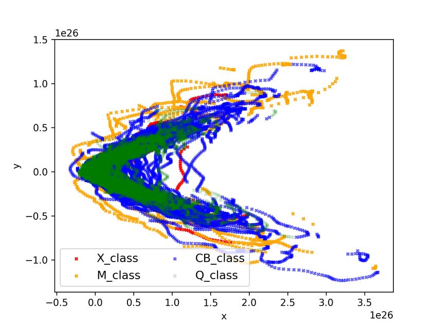
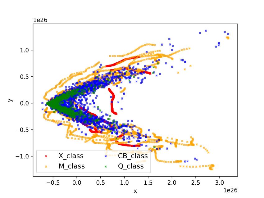
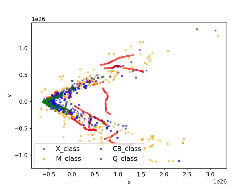
xi

 LIST OF FIGURES

Figure Page

 1.1 M class solar flare captured by NASA’s SDO. Image Credit: NASA/SDO . 3

 1.2 Image Credit: [1] Levels of solar flares as measured by GOES satellite near
 Earth . . . . . . . . . . . . . . . . . . . . . . . . . . . . . . . . . . . . . . . 4

 2.1 This image shows the three main SDO instruments on-board: AIA, HMI,
 EVE. HMI is responsible for capturing solar magnetic field information and
 the primary source of AR parameters that we feed to the classifiers to train
 and test. Image credits: NASA . . . . . . . . . . . . . . . . . . . . . . . . . 10

 2.2 The picture shows the observation window, which we feed to our classification
 models to predict the flare occurrence in the prediction period. In our case,
 the span of the observation window and the prediction window is 12 hours
 and 24 hours, respectively. Latency is minimized to the smallest possible
 time interval (the last point of the observation period is closest to the first
 point of the prediction period). Image Credits: [1] . . . . . . . . . . . . . . 11

 2.3 The flow of information from several sources and cross checking before arriv-
 ing at the final MVTS dataset ready for machine learning. Image Credits: [1] 12

 2.4 Flare class distribution showing the huge class imbalance . . . . . . . . . . 13

 2.5 2-D projections of the original and derived data sets to visualize the separabil-
 ity between the data samples of each class. It looks quite obvious that classes
 are not linearly separable. The SMOTE plus random under sampling dataset
 has over-sampled X class and under-sampled C/B and Q classes while the
 random under sampling dataset has under-sampled M, C/B and Q classes.
 Also shows that the derived data sets have done decent job in maintaining
 the original distribution. . . . . . . . . . . . . . . . . . . . . . . . . . . . . . 16

 2.6 Mutual Information scores of individual AR parameters, the red line is our
 threshold below which we doubt the contribution of the feature. . . . . . . . 19

 2.7 Random Forest Performance on individual AR parameters, it shows the same
 features as mutual information test as low performing except for MEANGBH. 21

 2.8 Neural Network Performance on individual AR parameters, it shows the same
 features as mutual information test as low performing except for MEANGBH. 21
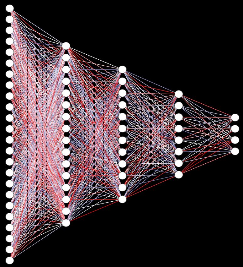
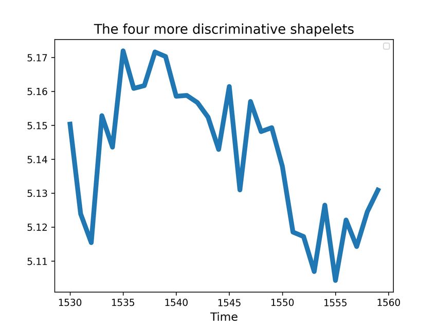
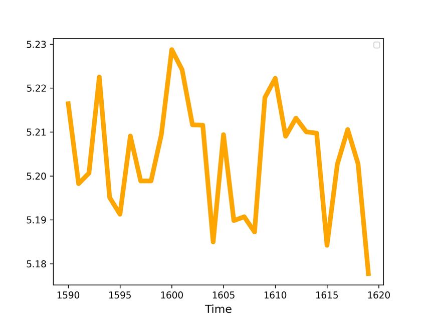
xii

2.9 Backward recursive feature elimination showing that the Random Forest
 model achieved the peak accuracy of 80.1% when four features are removed 22

3.1 Confusion Matrix . . . . . . . . . . . . . . . . . . . . . . . . . . . . . . . . . 26

3.2 ANN architecture that achieved the best performance . . . . . . . . . . . . 32

3.3 CNN architecture that achieved the best performance . . . . . . . . . . . . 33

3.4 LSTM architecture that achieved the best performance, image on the left
 side is the internal structure of LSTM unit. . . . . . . . . . . . . . . . . . . 34

3.5 Time series Forest algorithm; explains how each time series is transformed
 into a compressed feature space using a interval based approach and fed to
 the random forest . . . . . . . . . . . . . . . . . . . . . . . . . . . . . . . . . 36

3.6 Symbolic Aggregate Approximation and Vector Space Model; explains how
 the SAX dictionary of dataset in obtained based on which SAX term fre-
 quency vector of each class is derived. . . . . . . . . . . . . . . . . . . . . . 37

3.7 Shapelet based classification Algorithm; explains how the shapelets are ex-
 tracted from the time series dataset and best alignment distance matrix is
 obtained to train a kNN dataset. . . . . . . . . . . . . . . . . . . . . . . . 39

4.1 Classifiers across stratified 10-fold cross validation setting. Smaller box plots
 represent more consistent performance of classifier and larger ones represent
 the inconsistency in performance in different folds. . . . . . . . . . . . . . . 42

4.2 Class confusion matrix of the neural networks in median performing fold . . 43

4.3 Class confusion matrix of the time series classifiers in median performing fold 44

4.4 Time series forests performance on varying the number of decision trees . . 45

4.5 Most discriminative shapelet of each class based on shapelet transforms.
 Corresponding AR features from which these shapelets are extracted are
 RBT VALUE, RBP VALUE, RBZ VALUE, TOTPOT for X, M, CB and Q
 respectively. The graph represents value of the feature on y axis at a given
 time interval on x axis . . . . . . . . . . . . . . . . . . . . . . . . . . . . . . 46

4.6 Class confusion matrix of the baseline classifiers in median performing fold 47

4.7 Above line chart shows us the performance of ensemble with number of clas-
 sifier in x-axis. Starting with all the models in ensemble, we removed one by
 one based on TSS as priority. We achieved the best TSS with top 6 classifiers
 in the ensemble. . . . . . . . . . . . . . . . . . . . . . . . . . . . . . . . . . 48
xiii

4.8 Confusion matrix representing the reduced False alarm rate in the ensemble
 model classifier. . . . . . . . . . . . . . . . . . . . . . . . . . . . . . . . . . . 49

4.9 The Bar chart clearly shows that ensemble has successfully helped TSF to
 improve its performance on CB and Q class flares while X and M class per-
 formance is unaffected. . . . . . . . . . . . . . . . . . . . . . . . . . . . . . . 49

4.10 Statistical significance diagram of the solar flare prediction classifiers . . . . 51

4.11 Classifiers across stratified 10-fold cross validation setting on SMOTE RUS
 dataset. Smaller box plots represent more consistent performance of classifier
 and larger ones represent the inconsistency in performance in different folds. 52

4.12 Class confusion matrix of the neural networks in median performing fold . . 54

4.13 Class confusion matrices comparison of TSF between SMOTE and RUS
 datasets. . . . . . . . . . . . . . . . . . . . . . . . . . . . . . . . . . . . . . . 55

4.14 Class confusion matrix of the random forests and SVM in median performing
 fold . . . . . . . . . . . . . . . . . . . . . . . . . . . . . . . . . . . . . . . . . 55

4.15 Statistical significance diagram of the solar flare prediction classifiers . . . . 57
xiv

 ACRONYMS

MVTS Multivariate Time Series
AR Active Region
SDO Solar Dynamics Laboratory
NASA National Aeronautics and Space Administration
CME Coronal Mass Ejections
GOES Geostationary Operational Environmental Satellite
NOAA National Oceanic and Atmospheric Administration
SHARP Space weather HMI active region patch
HMI Helioseismic Magnetic Imager
PCA Principal component Analysis
TSF Time Series Forest
RF Random Forest
SVM Support Vector Machine
LSTM Long Short Term Memory
RNN Recurrent Neural Network
SAXVSM Symbolic Aggregate Approximation and Vector Space Model
ANN Artificial Neural Network
CNN Convolutional Neural Network
SMOTE Synthetic minority oversampling technique
CHAPTER 1

 INTRODUCTION

 The Sun has a massive impact on our planet and space behavior. Many changes, dis-

turbances, and phenomena keep occurring in and around the Sun’s atmosphere, generally

referred to as Solar activity. It has several variables that fluctuate even on a fraction of

a millisecond. There are four primary forms of solar activity: solar flares, coronal mass

ejections, high-speed solar winds, and solar energetic particles. While each of these forms

can negatively impact the earth, X-, M- solar flares and coronal mass ejections can disrupt

all earthly technologies, space architectures, destroy power grids, and pose radiation haz-

ards [2]. While posing such a significant threat, these extreme events are very rare, making

the prediction task very challenging.

 With the goal of understanding the influence of sun on earth’s behavior they launched

a Solar dynamics observatory mission in 2010. It continuously observes the sun’s magnetic

field and structure and tries to unfold how such huge amounts of energy is accumulated

and released in the form of solar winds into heliosphere and geospace. Although several

research communities are utilizing this information to explain the occurrence of flares, no

theory was able to certainly explain the mechanism behind them; which is hampering the

efforts to forecast. Meanwhile, with the growth in artificial data intelligence, space weather

strategies are drifting towards data driven approaches to find an efficient way.

 Our thesis attempts to help space weather forecasters predict solar flares occurring in

next 24 hours using machine learning techniques. We trained and evaluated nine machine

learning models to create a baseline for flare prediction tasks using a multivariate time series

(MVTS) dataset. Following are the classification models implemented in this thesis: fully

connected neural networks, convolutional neural networks [3], long short term memory net-
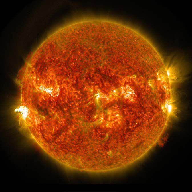
2

works, symbolic aggregate approXimation vector space model, time series forests, random

forests, shapelet transforms, support vector machines and logistic regression.

1.1 What are Solar flares?

 Solar flares are massive eruptions of electromagnetic radiation from the sun’s surface.

They originate from the release of high energy accumulated in the magnetic field of solar ac-

tive regions. When such areas suddenly explode they travel straight out from the flare sight

with incredible velocity in the form of solar winds. If the flare sight is facing the earth,

then there is a possibility that it can reach the earth’s atmosphere or human-interested

space. Nevertheless, when these solar flares are accompanied by large clouds of plasma and

magnetic field explosions called coronal mass ejections (CME) [4], they get splattered. They

can travel in any direction causing high-speed solar storms. An image of an evident solar

flare captured on August 24, 2014, by NASA’s solar dynamics observatory is displayed in

figure 1.1

 Solar flares are classified into five different levels based on their peak x-ray flux. The

figure 1.2 is the snapshot of 2 days from the GOES satellite observation where there is an

instance of X and M class flares. They are A, B, C, M, X classes, starting from A, each class

increases ten-fold in intensity. Most intense X and M class flares cause significant risk to

humans. In contrast, other flares can hardly impact human interests but can play a major

role in studying behavior of sun’s atmosphere.

1.2 Why do we need to predict Solar Flares?

 Intense enough Solar flares and CMEs, when they reach the earth’s atmosphere or

human interested space regions, can derange telecommunications, machinery, computers,

electrical appliances, etc., and can even blackout the earth. The airline passengers and

crew, astronauts in the space, space infrastructure, and satellites are at huge risk to such

flares [5].
3

 Fig. 1.1: M class solar flare captured by NASA’s SDO. Image Credit: NASA/SDO

 The sun goes through a solar cycle of 11 years, during which its activity decreases and

increases. Usually, when the activity ramps up, frequent massive solar flares and CMEs

occur, and chances that our planet can come in its way increases. However, flares hitting

the earth’s atmosphere are sporadic, but there are several instances in the last decade where

the earth has faced severe consequences. There were also cases where the earth could have

been wreak havoc if not for mere luck.

1.3 Few Instances when Solar flares hit the earth

 • July 23, 2012, when earth made a narrow escape

 An unusually large solar flare(CME) has hit NASA’s solar-terrestrial relations Obser-

 vatory satellite (STEREO) spacecraft that orbits the sun. As it was placed in orbit

 to observe and withstand such storms and flares, it survived the encounter. However,
4

Fig. 1.2: Image Credit: [1] Levels of solar flares as measured by GOES satellite near Earth

 when scientists calculated its occurrence, they realized that the earth had missed it

 by a margin of 9 days. Later in 2014, they have estimated that if a similar flare had

 occurred at that time, it would have caused cataclysmic damage worth $2 trillion,

 cost years to repair, and left people with the void of electricity.

 • March 10, 1989, when North America faced a blackout.

 A powerful CME has caused electric currents on the grounds of North America. It has

 created chaos by affecting around 200 power grids in Quebec, Canada, which resulted

 in 12 hr blackout. It interfered with sensors on the space shuttle Discovery and

 disrupted communication with satellites in space. In 1989, we encountered two other

 storms, one of which crashed computer hard drives halting Toronto’s stock market for

 few hours, and the other posed a life risk to astronauts causing burning in their eyes.

 • May 23, 1967, when United States thought it’s Russia.

 A large Solar flare has jammed the U.S. and United Kingdom’s radar and radio com-

 munications. The U.S. military has begun preparing for war, suspecting the soviets

 for the failure in communication systems; Just in time, space weather forecasters have

 intervened.

 Predicting the solar flares upfront may not help us to avoid the storms but could help

us in mitigating the damage by taking necessary precautions. As humans are now are
5

exploring space more than ever and becoming more and more technology and electricity-

dependent, the risk the flares could pose to humans is shooting up [2]. Therefore, continuous

monitoring of solar events is crucial for accurately forecasting space weather. NOAA has

a constellation of geostationary operational environmental Satellites which send continuous

stream of data to support the weather forecasting, solar events tracking and other research.

However, the mechanism behind their occurrence is still not completely known.

 As the understanding of theoretical models of solar flare events such as the relationship

between the photospheric and coronal magnetic field is limited, the heliophysics community

is showing an inclination towards data-driven approaches to replace the expensive setup [5].

Note: Information and facts about solar flares presented in this thesis have been taken

from the web sources of NASA, NOAA, SDO.

1.4 What is the existing knowledge?

 This section summarizes our study of the already established knowledge of flare predic-

tion studies. Significantly, the prediction pipelines that were built using machine learning

models. Most of the approaches were data-driven except for the rule-based expert system

called THEO by Mcintosh [6] in the earlier days of flare prediction in 1990. Also, most of

the earlier studies did not consider the data’s time-series nature.

 Initial data-driven approaches were based on linear statistical modeling. In the work

of Jing [7], they tried to find the correlations between the magnetic parameters and a flare

production based on line of sight vector magnetogram data. Later on, several machine

learning approaches were implemented using the vector magnetogram data. Below is the

list of Machine learning techniques that have been experimented on in this task.

 • Time series Forest(TSF) (2020) [8] They took a contrasting approach; they tried to

 predict if the forecasts flare-free or not while trying to minimize the number of false

 negatives and false alarms. They trained the interval based model called TSF, which
6

 uses a random forest classifier to make the prediction. They achieved able to detect

 non-flaring activity with a recall of 88.5%.

• Solar flare prediction using LSTM network (2020) [9] They reduced the flare prediction

 problem to binary classification and used 20 SHARP parameters to train an LSTM

 network. A TSS of 0.79 has been achieved in identifying flares ≥ M. They concluded

 that SHARP parameters have limited information.

• Gramian Angular Fields Images using Neural Networks (2018) [10]

 This research converted the time series X-ray data acquired from the GOES satellite

 into Gramian angular field images to train a convolutional neural network after com-

 pressing the data using a piece-wise approximation. However, their results were not

 impressive.

• k-NN based on Time series data (2017) [5]

 This study performed their experiments using a k-NN classifier with the vector mag-

 netogram time-series data. They compared each of the 16 univariate feature’s perfor-

 mance before concluding that ”TOTUSJH” is the best AR parameter with a flaring

 region recall of 90% .

• Multivariate Time Series Decision Trees (2017) [11] This research has approached

 this problem using multivariate time series analysis perspective to cluster potential

 flaring active regions by applying distance clustering [12–15] to each feature and then

 organizing them back together into a multivariate time series decision tree. They

 achieved an accuracy of 85% in predicting the flaring activity.

• k-NN and ERT (Extremely randomized tree) (2017) [16]

 This research combined the line of sight data, vector magnetogram data, GOES X-

 ray data and UV continuum of the lower chromosphere from atmospheric imaging

 assembly to calculate 65 features. They trained three machine learning algorithms:

 SVM, k-NN, and ERT, to achieve the true skill score of 0.9. (Skill scores will be

 explained in the later section)
7

 • Support Vector Machines (2015) [17] Their attempt to forecast the X- and M- flares

 relied on the 25 AR vector magnetogram features. They calculated the linear cor-

 relation between each feature and target variable to eliminate 12 features from their

 forecasting algorithm. They achieved a TSS skill score of 0.61 with the SVM algo-

 rithm.

 Apart from the above-mentioned notable research on Flare prediction, more research

is performed on this task in a data-driven approach. Right from 2001 to 2015 several ma-

chine learning algorithms were experimented to improve flare prediction; such as pattern

recognition using relevance vector machine by Al-Ghraibah [18], cascade correlation Neural

Networks by Ahmed [19], logistic regression by Y.Yuan [20], decision trees by D.Yu [21] and

artificial neural networks by R.A.F. Borda [22].

 Based on our literature study, we observed that the time-series nature of vector magne-

togram data is not yet well studied except for the works of Angryk [11], [8], where they used

time-series forest and multivariate decision trees. Secondly, the flare prediction problem is

modeled chiefly as a binary classification problem. They combined X and M class flares as

positive classes and C, B, Q as the negative class. Though binary modeling fulfills the main

objective of identifying the most harmful flares, they ignore the importance of C and B class

flares, completely treating them as non-flaring events. According to a study [23], C class

flares are more valuable than X and M class flares in studying the evolution of sunspots.

Furthermore, B class flares are more synchronous with sunspot group numbers than X and

M when the number of sunspot groups is around 100. This study concludes C and B as low

magnetic activity flares that could be crucial in studying the sunspot groups, which are the

main cause of solar flares. Though there are a different variety of machine learning models

experimented there is no common dataset that has been investigated on all of them to find

the classifier that is the most suitable for this prediction task.
8

 Considering the above-discussed points, our thesis aims to make an extensive com-

parison of different types of Neural Network architectures and time-series classifiers and

the baseline comparison with traditional classifiers such as Random Forests, SVM, logistic

regression. We modeled the problem as a 4 class problem to classify the flares between

X, M, C/B, and Q classes. We hope that this contribution will be a valuable asset to the

data-driven flare prediction community and fills a few gaps in this area’s existing knowledge.

1.5 Thesis Organization

 • Chapter 2: Introduction to the dataset, explains where the data is coming from and

 what are the features present, how much data we have and the challenges it brings

 and the feature selection pipeline used to arrive at the final dataset.

 • Chapter 3: In this chapter, we discuss machine learning methodologies used in different

 experiments and the evaluation techniques used in our thesis including the domain

 specific metrics.

 • Chapter 4: Here, we describe and discuss the results achieved in the experiments and

 compare the performance of classifiers.

 • Chapter 5: In the final chapter, we discuss the outcomes, conclusions, challenges and

 future scope of this thesis.
9 CHAPTER 2 DATA ANALYSIS AND FEATURE SELECTION 2.1 Introduction to the Dataset A Time series is a progression of a variable feature captured in continuous time intervals. The spacing between each time instance (τ ) captured is known as cadence. Our dataset is time-series data with a cadence of 12 minutes through 60 time intervals (60τ , 12 hours long). As our data has multiple variable features (33), it is called as Multivariate Time series data. The below matrix represents the dimension of our sample. Each sample of our data consists of 33 active region magnetic field parameters ac- quired from HMI instrument on solar dynamics observatory. Each feature is a time-series of mathematically represented magnetic field parameter. The table 2.2 below is the list of features and their description. More information about each feature can found at: ”http://jsoc.stanford.edu/doc/data/hmi/sharp/sharp.htm”. f1,1 f1,2 f1,3 f1,4 ··· f1,60 f2,1 f2,2 f2,3 f2,4 · · · f2,60 M V T S(33,60) = . . .. .. .. .. .. . . . . . . f33,1 f33,2 f33,3 f33,4 · · · f33,60 2.2 Data Acquisition Solar flares and CMEs occur in the Sun areas where there is a strong magnetic field. Such areas are called flaring Active regions(AR). Though the underlying mechanism of how solar flares and CMEs occur is still not well understood, there are several studies that show solar flares arise because of sudden release of energy developed by photospheric magnetic reconnection in the coronal field [24]. This is well known as CSHKP model; there are sev- eral other variations of these models explaining the initiation mechanisms of the flares and
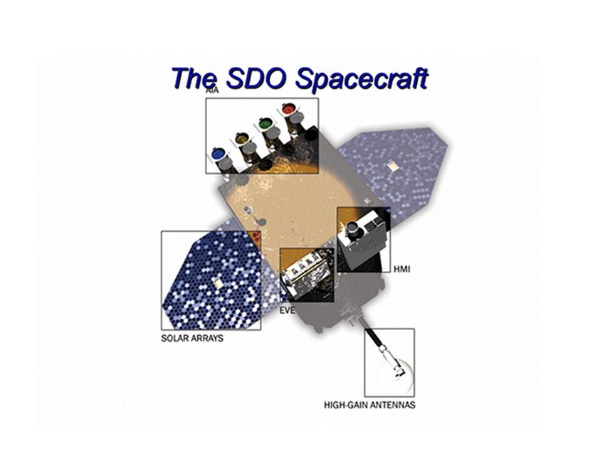
10

CMEs. Since the photospheric magnetic field has a huge role in driving the coronal field

around the Sun, it is highly possible that evolution patterns of the photospheric magnetic

field may serve as indicators for predicting solar flares and CMEs.

 The solar dynamic observatory satellite that has been launched by NASA a few years

ago has been observing the Sun from 2010. It has three instruments set up on board

for different purposes: Extreme Ultraviolet Variability Experiment (EVE), Helioseismic

and Magnetic Imager (HMI) and Atmospheric Imaging Assembly (AIA). HMI takes the

high-resolution measurement of photospheric vector magnetic field parameters and extracts

space weather HMI AR patches (SHARPS). [25] AIA is responsible for imaging the outer

surface(corona) of the sun, it captures full sun images every 10 seconds. EVE keeps track of

extreme ultraviolet rays and helps us in calculating the amount of UV reaching the earth.

Fig. 2.1: This image shows the three main SDO instruments on-board: AIA, HMI, EVE.
HMI is responsible for capturing solar magnetic field information and the primary source
of AR parameters that we feed to the classifiers to train and test. Image credits: NASA
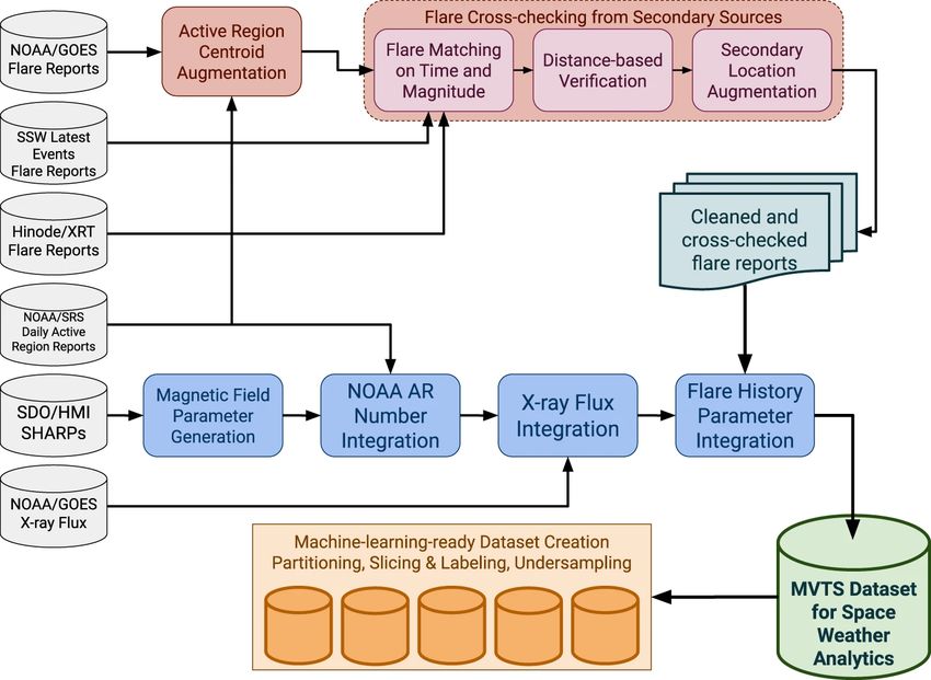
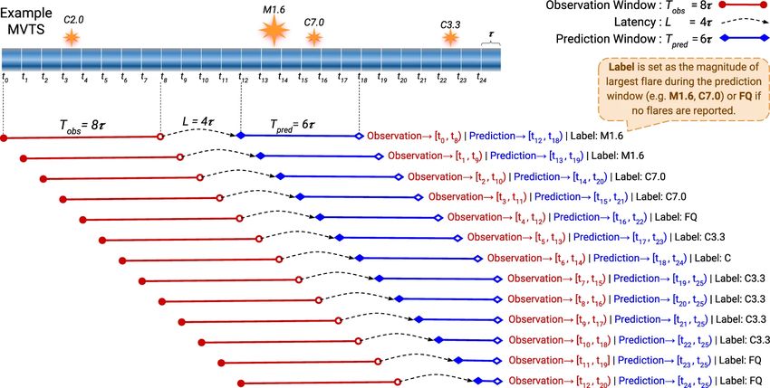
11

 In our thesis, the data we are using is coming from the HMI called SHARPS. They

have several pre-calculated time series quantities(AR parameters) captured by HMI every

12 minutes. These quantities called as active region (AR) parameters, and are our features

in the each sample 2.2. Each time series is a look back of flare or no flare occurrence.

Similar to the work of Bobra and Couvidat [17] we are using these past observations of AR

parameters as preflare signatures to train the AI models to predict future flaring activity.

These long SHARP time series are broken into chunks of 60 instances of span 12 hours,

making our multivariate time series dataset. The label of each MVTS is the largest flare

that occurred in next 12 hours (prediction period).

Fig. 2.2: The picture shows the observation window, which we feed to our classification
models to predict the flare occurrence in the prediction period. In our case, the span of
the observation window and the prediction window is 12 hours and 24 hours, respectively.
Latency is minimized to the smallest possible time interval (the last point of the observation
period is closest to the first point of the prediction period). Image Credits: [1]

 The MVTS dataset was made available by a research team from Georgia State Univer-

sity. This dataset was made with an intention to facilitate machine learning models. The

labels for each time series are also marked with utmost care after several phases of clean-

ing, pre-processing and cross checking with secondary sources. The block diagram briefly
12

mentions the cleaning phases and secondary data sources 2.3. Much detailed information

about AR parameters and the dataset can be found at [1].

Fig. 2.3: The flow of information from several sources and cross checking before arriving at
the final MVTS dataset ready for machine learning. Image Credits: [1]

2.3 Datasets

 On the Georgia state university public server, the latest flare dataset is available. They

have three partitions of data that are labeled. There are a total of 214023 MVTS, out of

which only 1.98% of them are from X- and M- preflare signatures and 82.64% are flaring

quiet regions (Q class), and the remaining are C and B class preflare signatures 2.1. The

dataset excluded A class flare data as they do not pose any risk and are have almost

negligible peak flux.

Datasource: https://dmlab.cs.gsu.edu/solar/data/data-comp-2020/
13

 Fig. 2.4: Flare class distribution showing the huge class imbalance

 Classes/Partition X M C B Q
 P1 172 1157 6531 6010 63400
 P2 72 1393 9130 5159 78013
 P3 141 1313 5364 709 35459
 Class % 0.179 1.80 9.82 5.54 82.64

 Table 2.1: Class Distribution across different data partitions

2.3.1 Class imbalance problem

 From the pie chart in figure 2.4 it’s explicit that we have fewer samples of the critical X-

and M- class flares. On the other hand, we have a ton of samples for non-flaring instances,

leaving us with class imbalance problem as high as 1 is to 800 between the minority X class

and majority Q class. Class imbalance problems can skew the models drastically, making

them biased to the classes with majority samples. On top of that, our majority class is

the negative flare class (Q) which implies that the model could end up with too many false

negatives (Increased chances of missing the flare detection) [26] .

 For the scope of this thesis, we decided to generate two data sets to experiment with

different machine learning models; one based on random under sampling and the other with
14

a combination of oversampling and under-sampling to tackle the class imbalance problem.

Note that we merged classes C and B as one class based on the discussion in the literature

study. Hence our two final data sets will be having X, M, C/B, and Q classes.

2.3.2 Random under-sampling

 We took the classic random under-sampling approach on the classes with more samples

to tackle this problem. In this method, we down-sample the majority classes to the minority

classes by randomly selecting the required number of samples to be included. While this

method looks very simple, we can’t overlook its success in addressing the class imbalance

in several applications [27]. Though random under-sampling might lead to the loss of

unique data, in most cases, it is proven to be advantageous and generalized better than

oversampling. In the study of Satwik Mishra [28], they compared SMOTE approach with

under-sampling on randomly generated data sets and found out that random under-sampling

is performing better with random forests and XGboost. Our under-sampled dataset has

1540 samples, with each of the majority classes down-sampled to 385 samples to be on par

with the minority X- class. This dataset will be referred as RUS dataset in the rest of the

thesis.

2.3.3 SMOTE along with random under-sampling

 However, we can not say that one specific approach would work with this applica-

tion. Hence, we did not wholly overlook the oversampling approach, as it is advantageous

to accommodate more data for data-hungry models like neural networks. We arrived at

a hybrid method that includes oversampling the minority class by SMOTE and random

under-sampling of majority classes.

 Synthetic minority oversampling (SMOTE) over samples the minority class by generat-

ing synthetic samples, unlike oversampling by replicating data. SMOTE operates on feature

space instead of data space; it uses the kNN approach [29] and creates new samples on the

line segment, joins all or any of the k nearest neighbors based on the chosen oversampling
15

rate. [30] In our case, we over-sampled the X- class and down-sampled C/B and Q classes

to the level of M- class. This brings our dataset to the size of 15440 with 3860 samples in

each category. This dataset will be referred as SMOTE RUS dataset in rest of the thesis.

 To get a general idea about how well the data of each class is separated, we used

principal component analysis (PCA) to project the original dataset in a two-dimensional

plane. PCA computes principal components by performing eigen decomposition on the

covariance matrix of the features from the dataset while minimizing the loss of information.

Looking at the figure 2.5, we can undoubtedly say that the data is not linearly separable.

The figure shows the derived data sets their class distribution and projection in the 2-D

feature space.
16

 Original Dataset

 Class X M C/B Q
 Samples 385 3860 32903 176872

 SMOTE (X) + Random under sampling (C/B, Q) Random under sampling (M, C/B, Q)
 (SMOTE_RUS) (RUS)

 Class X M C/B Q Class X M C/B Q
 Samples 3860 3860 3860 3860 Samples 385 385 385 385

Fig. 2.5: 2-D projections of the original and derived data sets to visualize the separability
between the data samples of each class. It looks quite obvious that classes are not linearly
separable. The SMOTE plus random under sampling dataset has over-sampled X class and
under-sampled C/B and Q classes while the random under sampling dataset has under-
sampled M, C/B and Q classes. Also shows that the derived data sets have done decent
job in maintaining the original distribution.
17

 ID AR Parameter Description
 0 TOTUSJH Total unsigned current helicity
 1 TOTBSQ Total magnitude of Lorentz force
 2 TOTPOT Total photospheric magnetic energy density
 3 TOTUSJZ Total unsigned vertical current
 4 ABSNJZH Absolute value of the net current helicity in G2/m
 5 SAVNCPP Sum of the absolute value of the net current per polar-
 ity
 6 USFLUX Total unsigned flux in Maxwells
 7 TOTFZ Sum of Z-component of Lorentz force
 8 MEANPOT Mean photospheric excess magnetic energy density
 9 EPSZ Sum of Z-component of normalized Lorentz force
 10 SHRGT45 Area with shear angle greater than 45 degrees
 11 MEANSHR Mean shear angle
 12 MEANGAM Mean inclination angle
 13 MEANGBT Mean value of the total field gradient
 14 MEANGBZ Mean value of the vertical field gradient
 15 MEANGBH Mean value of the horizontal field gradient
 16 MEANJZH Mean current helicity
 17 TOTFY Sum of Y-component of Lorentz force
 18 MEANJZD Mean vertical current density
 19 MEANALP Mean twist parameter
 20 TOTFX Sum of X-component of Lorentz force
 21 EPSY Sum of Y-component of normalized Lorentz force
 22 EPSX Sum of X-component of normalized Lorentz force
 23 R VALUE Total unsigned flux around high gradient polarity in-
 version lines using the Br component
 24 RBZ VALUE Derived
 25 RBT VALUE Derived
 26 RBP VALUE Derived
 27 FDIM Derived
 28 BZ FDIM Derived
 29 BT FDIM Derived
 30 BP FDIM Derived
 31 PIL LEN Derived
 32 XR MAX Derived

Table 2.2: 33 Active region magnetic field parameters which are our features in multivariate
time series dataset. Each of these parameter is a time-series captured with a cadence of 12
minutes. Our MVTS dataset has 60 instances of each feature in every sample
18

2.4 Data preprocessing

 As the dataset is thoroughly validated and made machine learning ready [1], we only

made the basic checks, such as imputing the missing values and removing the outliers. We

filled them with the corresponding feature’s mean in the time series with missing values.

We got rid of the XR MAX feature as it consisted of many outliers and its univariate per-

formance was also very poor. Univariate performance evaluation is discussed in the next

section.

 The AR features have values ranging in different scales and huge magnitudes. Hence,

each feature has been z-normalized (standard score) across the dataset before sending them

as input to the machine learning models. Standard score normalization allows us to compare

raw scores from two different normal distributions while considering both mean values and

variance. In our experiments, Z-normalization helped neural networks avoid exploding

gradient problems and speed up the computation by reducing rounding errors and expensive

operations.

2.5 Feature Selection

 Now that we have our data samples ready and classes are finalized we can now jump

into feature selection. In this section we aimed to quantify the importance of features using

few statistical and performance based tests. Based on our tests few features turned out to

be useless and only added noise to the ML systems. To calculate each feature’s contribution,

we performed a statistical test, which is independent of the machine learning models and

two machine learning-based performance tests using Random Forests and Convolutional

Neural Networks. Our goal here was to find the best-performing minimal feature set.

 Our focus in this feature selection pipeline was to quantify the univariate importance

of derived parameters that introduced each parameter’s weighting based on their distance

from the polarity inversion line on the active region the parameter were collected. As these

parameters were experimental, their contribution to the models is skeptical.
19

 • Mutual Information Analysis: Mutual Information between two variables captures

 both linear and non-linear relationships. For example, if X and Y are two variables,

 let us take X as one of the 33 features and Y as our target class (X- flare). Suppose

 X and Y are independent variables, then the mutual information score will be 0. If

 there exists a deterministic function between X and Y, then the mutual information

 score will be one. For other cases, mutual Information will be between 0 and 1. The

 below bar chart shows us where each feature stands based on the mutual information

 2.6.

Fig. 2.6: Mutual Information scores of individual AR parameters, the red line is our thresh-
old below which we doubt the contribution of the feature.
20

 The following five features were on the radar to be removed as their mutual information

 contribution is limited and under the lenient threshold of 0.1

 – FDIM

 – BZ FDIM

 – BP FDIM

 – BT FDIM

 – MEANGBH

 However, before removing these features to get more evidence and confirm that these

features are underperforming or not adding any value to the remaining features, we have

run experiments on each univariate feature with random forest and convolutional neural

networks to rank the features based on classification performance.

 A simple convolutional neural network with 4 and 8 filters and a random forest with

50 decision trees has been trained with each univariate feature individually. Performance

results are captured by training and testing the models using 10-fold cross-validation. The

results in figures 2.8 and 2.7 show that four of the five features sidelined based on mutual

information scores also appeared here at the table’s bottom except for the MEANGBH

feature.

 As a final step in our feature selection process, we performed a backward recursive

feature elimination technique to ensure that the removal of the features is not affecting the

classification performance. In this procedure, we remove the low-priority features one by

one based on a priority order until there is only the highest priority feature left. Ideally,

this test plots an elbow curve showing the peak value at an optimal number of features.
21

Fig. 2.7: Random Forest Performance on individual AR parameters, it shows the same
features as mutual information test as low performing except for MEANGBH.

Fig. 2.8: Neural Network Performance on individual AR parameters, it shows the same
features as mutual information test as low performing except for MEANGBH.
22

 Stating that our hypothesis of removing the four features (FDIM, BZ FDIM, BP FDIM,

BT FDIM) is true, the elbow curve has peaked when these four features are removed from

the dataset. We have implemented this backward recursive feature elimination on random

forests and neural networks.The fig 2.9 and table 2.3 shows the results of these tests.

Fig. 2.9: Backward recursive feature elimination showing that the Random Forest model
achieved the peak accuracy of 80.1% when four features are removed

 Metric\Number of Features 32 28 27 20 14
 Accuracy 0.785 0.795 0.770 0.735 0.729
 HSS1 0.570 0.591 0.541 0.471 0.458
 HSS2 0.701 0.717 0.681 0.627 0.618
 TSS 0.703 0.718 0.682 0.629 0.621

Table 2.3: Performance metrics of neural networks with number of features as variable. Left
to right features are removed based on the mutual information priority. With 28 features
the neural networks gave ts peak performance.
23

 Based on the above experiments, we can say that model performance has slightly in-

creased with removing features; adding those four features does not benefit. Hence, we

decided to remove the four features FDIM, BZ FDIM, BP FDIM, BT FDIM, along with

the XR MAX, which is causing outliers. The final datasets (RUS and SMOTE RUS) we are

going to use for implementing machine learning models will have a reduced feature space

of 28 features instead of 33.
24

 CHAPTER 3

 METHODS AND EXPERIMENTS

 As we now developed a thorough understanding of the solar flare prediction prob-

lem and the data sets. This chapter will discuss machine learning algorithms that were

used in our experiments along with training and testing strategies and performance eval-

uation techniques. All the experiments in thesis can be classified as RUS based and

SMOTE RUS based. First we experimented on different machine learning models using

the RUS dataset and next the top six performing architectures/models were experimented

using the SMOTE RUS dataset. The chapter will be structured as mentioned below.

 • Performance Evaluation Metrics

 • Training and Testing Strategy

 • Traditional Machine learning Algorithms:

 – Logistic Regression

 – Support Vector Machines

 – Random Forests

 • Neural Network Architectures:

 – Multi layer Perceptron (MCP)

 – Recurrent Neural Networks with Long short term memory(LSTM) units

 – Convolutional Neural Networks

 • Time Series Classifiers:

 – Time Series Forest

 – Symbolic Aggregate approXimation (SAX) Vector space model (VSM)

 – Shapelet Transforms
25

3.1 Performance Evaluation Metrics

 Metrics help analyze the performance of the model. After data cleaning, Feature se-

lection, and training the model, we get the results as a probability or class. It’s essential

that we choose the right metrics to evaluate our models based on the nature of the data,

such as the consequences of false negatives or false positives. For example, In a model that

tells us whether to buy a specific stock, we can’t afford a false positive because investing in

an unprofitable venture leads you to lose. Hence, in this case, precision is more important

than recall. Similarly, in COVID detection, false negatives can’t be tolerated as they pose

a massive risk to the patients and other people in contact with the person. Hence, in this

case, the recall will be our chosen metric.

 In Solar Flare prediction, the false negatives can cause crucial damage to the earth and

space resources; consequences such as satellite destruction or collapse of power grids may

occur, while false positives can also trigger satellite maneuvering or expensive preventive

measures. However, not detecting the flares will definitely because more damage than false

alarms. Hence recall of flaring activity will be crucial in deciding the suitable model. Below

are the standard metrics we are using to evaluate our models.

 As our prediction has more than two outcomes, we followed the one vs. rest procedure

to find performance measures for each class and then calculated the weighted average to

find the metric for the model as a whole. The following quantities required to calculate

metrics are captured from confusion matrix 3.1.

 • True Positives (TP) and False Positives (FP)

 • True Negatives (TN) and False Negatives (FN)

 • Positives (P) and Negatives (N)

 • Predicted Positives (P’) and Predicted Negatives (N’)
26

 Predictions

 Target Class Rest Total

 Target Class TP FN P
 Actuals
 Rest FP TN N

 Total P’ N’ P+N

 Fig. 3.1: Confusion Matrix

 • The Recall represents the models ability to classify a positive class as positive.

 TP
 TP + FN

 • The Precision represents the model’s ability to not classify a negative class as positive.

 TP
 TP + FP

 • The F1-score is the harmonic mean of precision and recall of a classifier. This metric

 comes into picture when you can’t decide upon choosing a model based on recall or

 precision.
 2 ∗ P recision ∗ Recall
 P recision + Recall

 • The Accuracy allows us to quantify the total number of correct predictions made by

 a classifier. This metric often fails to handle the class imbalance problem as it gets

 biased to the class with more samples.

 TP + TN
 TP + TN + FP + FN

 Except for the recall of other metrics, the metrics mentioned above are not very suit-

able for this task. Hence, we decided to calculate skill scores [31] which are being widely
27

used by the solar flare prediction community [17] [16] [5]. They are the following:

 • Heidke Skill Scores (HSS) is present in two versions; HSS1 is defined by Leka and

 Barnes [32]; it ranges from −∞ to 1. A score closer to 1 represents a perfect forecast,

 while 0 illustrates that the model predicted everything as a negative class. While

 negative scores denote that performance is worse than anticipating everything under

 negative class. It measures forecast over predicting that no flare will ever occur. This

 measure makes sense, as solar flares are rare events.

 TP + TN − N
 HSS1 =
 P

 HSS2 is another skill score which measures the improvement of prediction over random

 predictions [5] [33]. This metric is defined by the Space weather prediction center. [17]

 Score ranges from 0 to 1; closer to one better the forecast.

 2 ∗ [(T P ∗ T N ) − (F N ∗ F P )]
 HSS2 =
 P ∗ N0 + N ∗ P0

 • Gilbert Skill Score (GS) [5] [33] takes True positives obtained by chance into con-

 sideration. This helps one to arrive at model which is not predicting the flares by

 chance.
 0
 T P ∗ (P + N ) − P ∗ P
 GS =
 F N ∗ (P + N ) − N ∗ P 0

 • True Skill Statistic (TSS) is a metric independent of the class imbalance ratio. This

 is the most desired metric in the solar flare prediction community, as it converges to 1

 when the false alarm rate and the false-negative rate are minimized. Flare prediction

 demands a very similar metric; we neither want to create chaos unnecessarily or miss

 a flare and put humans at risk. [17] [34] [5].

 TP FP
 T SS = −
 P N
28

 Every skill score has its characteristic which can be helpful to analyze. However, HSS1,

HSS2, and GS are still somewhat prone to class imbalance ratio [5]. Hence, in the later

sections of results and discussion, we will be analyzing the performance more in terms of

TSS and Recall.

3.2 Training and testing strategies

 To handle the class imbalance problem, we have under-sampled our dataset to 1540

MVTS. As most machine learning models are data-hungry, standard train-test splits such

as 60-40 or 70-30 would leave the model with a shortage of data either for validation or

training. Hence, we decided to perform stratified 10-fold cross-validation.

 Stratified Cross-validation uses a stratified sampling technique to divide the data into

k folds. Stratified sampling ensures the same proportion of samples are present in each fold.

This method helps us to approximate the generalization error using cross-validation closely.

Also, no sample will be over or underrepresented in the training and testing sets. It follows

the below procedure:

 • Randomly Shuffles the entire dataset.

 • Splits the dataset into k groups with each group having same class concentration.

 • Every group is once held out as a testing group (Test Set).

 • Remaining groups are used to train the model (Train set).

 • Train the model with train set and evaluate with test set.

 • Re-initialize the model to train with all of the k combinations.

 • Performance of model is retained after evaluating model with each test set.
29

3.3 Traditional Classifiers

 We performed experiments on the traditional classifiers to establish a baseline for Neu-

ral Network models and Time series classifiers. These classifiers can handle only univariate

time series data. Hence, we flattened the 28 features into one extended feature vector,

partly sacrificing the time-series nature of the data following the work of Bobra [17] where

he used a similar kind of vector magnetogram data.

 Our task is a 4 class classification problem, and the class data is non-overlapping. The

train and Test Splits are z-score normalized for all the classifiers before flattening and send-

ing them as input. All the machine learning model implementations in this section are using

the Scikit-Learn library.

3.3.1 Support Vector Machines

 SVM is a supervised machine learning algorithm known for classification tasks. SVM

plots the N-dimensional data and aims to find the optimal (N-1) hyperplane possible that

can split the dataset into different groups [35]. If there are only two features, then the

hyperplane becomes a line. The two hyper-parameters we need to adjust are C, Gamma γ

and the kernel type. C is the penalty imposed for each misclassification; the lower the C, the

more tolerant to misclassifications and the better it generalizes. Gamma is the curvature

amount that we need to tune for only the RBF kernel.

 In our experiments with SVM we performed a grid search with C ranging from 0.0001

to 10 and gamma from 0.0001 to 1. We used this search space for rbf and poly except for

linear kernel which doesn’t need gamma to be adjusted. The radial basis function is our

best-performing kernel with a C value of 0.1 and Gamma of 0.01.
You can also read