Emergent relationships with respect to burned area in global satellite observations and fire-enabled vegetation models - Biogeosciences
←
→
Page content transcription
If your browser does not render page correctly, please read the page content below
Biogeosciences, 16, 57–76, 2019
https://doi.org/10.5194/bg-16-57-2019
© Author(s) 2019. This work is distributed under
the Creative Commons Attribution 4.0 License.

Emergent relationships with respect to burned area in global
satellite observations and fire-enabled vegetation models
Matthias Forkel1 , Niels Andela2 , Sandy P. Harrison3 , Gitta Lasslop4 , Margreet van Marle5 , Emilio Chuvieco6 ,
Wouter Dorigo1 , Matthew Forrest4 , Stijn Hantson7 , Angelika Heil8 , Fang Li9 , Joe Melton10 , Stephen Sitch11 ,
Chao Yue12 , and Almut Arneth13
1 Climate  and Environmental Remote Sensing Group, Department of Geodesy and Geoinformation,
Technische Universität Wien, Vienna, Austria
2 Biospheric Sciences Laboratory, NASA Goddard Space Flight Center, Greenbelt, MD, USA
3 Department of Geography and Environmental Science, University of Reading, Reading, UK
4 Senckenberg Biodiversity and Climate Research Centre, Frankfurt am Main, Germany
5 Deltares, Delft, the Netherlands
6 Environmental Remote Sensing Research Group, Department of Geology, Geography and the Environment,

Universidad de Alcalá, Alcalá de Henares, Spain
7 Geospatial Data Solutions Center, University of California, Irvine, CA, USA
8 Department for Atmospheric Chemistry, Max Planck Institute for Chemistry, Mainz, Germany
9 International Center for Climate and Environmental Sciences, Institute of Atmospheric Physics,

Chinese Academy of Sciences, Beijing, China
10 Climate Research Division, Environment Canada, Victoria, BC, Canada
11 College of Life and Environmental Sciences, University of Exeter, Exeter, UK
12 Laboratoire des Sciences du Climat et de l’Environnement, Gif-sur-Yvette, France
13 Atmospheric Environmental Research, Institute of Meteorology and Climate Research,

Karlsruhe Institute of Technology, Garmisch-Partenkirchen, Germany

Correspondence: Matthias Forkel (matthias.forkel@geo.tuwien.ac.at)

Received: 28 September 2018 – Discussion started: 18 October 2018
Revised: 5 December 2018 – Accepted: 11 December 2018 – Published: 11 January 2019

Abstract. Recent climate changes have increased fire-prone     and from DGVMs from the “Fire Modeling Intercompari-
weather conditions in many regions and have likely affected    son Project” (FireMIP) that were run using a common proto-
fire occurrence, which might impact ecosystem function-        col and forcing data sets. The satellite-derived relationships
ing, biogeochemical cycles, and society. Prediction of how     indicate strong sensitivity to climate variables (e.g. maxi-
fire impacts may change in the future is difficult because     mum temperature, number of wet days), vegetation proper-
of the complexity of the controls on fire occurrence and       ties (e.g. vegetation type, previous-season plant productivity
burned area. Here we aim to assess how process-based fire-     and leaf area, woody litter), and to socio-economic variables
enabled dynamic global vegetation models (DGVMs) rep-          (e.g. human population density). DGVMs broadly reproduce
resent relationships between controlling factors and burned    the relationships with climate variables and, for some mod-
area. We developed a pattern-oriented model evaluation ap-     els, with population density. Interestingly, satellite-derived
proach using the random forest (RF) algorithm to iden-         responses show a strong increase in burned area with an in-
tify emergent relationships between climate, vegetation, and   crease in previous-season leaf area index and plant produc-
socio-economic predictor variables and burned area. We ap-     tivity in most fire-prone ecosystems, which was largely un-
plied this approach to monthly burned area time series for     derestimated by most DGVMs. Hence, our pattern-oriented
the period from 2005 to 2011 from satellite observations       model evaluation approach allowed us to diagnose that veg-

Published by Copernicus Publications on behalf of the European Geosciences Union.
58 M. Forkel et al.: Emergent relationships with respect to burned area
etation effects on fire are a main deficiency regarding fire- 2018; Jolly et al., 2015; Müller et al., 2015); however, it has
enabled dynamic global vegetation models’ ability to accu- been suggested that changes in land use compensate for cli-
rately simulate the role of fire under global environmental mate effects and result, for example, in declining burned ar-
change. eas in African savannahs (Andela and van der Werf, 2014).
Hence, there is still uncertainty regarding factors such as
the cause of the recent observed decline in global burned
area (Andela et al., 2017). Furthermore, there is even greater
1 Introduction uncertainty about the potential trajectory of changes in fire
regimes in the future (Settele et al., 2014).
About 3 % of the global land area burns every year (Chu- Fire-enabled dynamic global vegetation models (DGVMs)
vieco et al., 2016; Giglio et al., 2013; Randerson et al., or Earth system models are process-oriented tools used to
2012). Fire represents a strong control on large-scale veg- predict the consequences of future climate change on fire
etation patterns and structure (Bond et al., 2004) and can regimes and associated feedbacks (Hantson et al., 2016). Our
significantly accelerate the impacts of changing climate or faith in these projections is contingent on the ability of these
land management on global ecosystems (Aragão et al., 2018; models to capture features of the current situation. State-of-
Beck et al., 2011). Fire directly affects global and regional the-art fire-enabled DGVMs partly capture the spatial pat-
climate through changing surface albedo (López-Saldaña et terns of burned area (Andela et al., 2017; Kelley et al., 2013);
al., 2015; Randerson et al., 2006), atmospheric trace gas, and however, doubt has been cast on the ability of these models
aerosol concentrations (Andreae and Merlet, 2001; Ward et to capture the response to extreme events and recent trends in
al., 2012), and on longer timescales by affecting vegetation burned area (Andela et al., 2017). This suggests that they in-
composition and structure with subsequent impacts on the accurately represent the response of fire to combined changes
carbon cycle and hydrology (Li and Lawrence, 2016; Pausas in climate, vegetation, and socio-economic drivers.
and Dantas, 2017; Tepley et al., 2018; Thonicke et al., 2001). Here we aim to test how fire-enabled DGVMs repro-
Climate influences several aspects of the fire regime, in- duce emergent relationships with the drivers of burned area.
cluding the seasonal timing of lightning ignitions (Veraver- We apply a machine learning algorithm to the output from
beke et al., 2017), temperature and moisture controls on seven fire-enabled DGVMs and a suite of satellite and other
fuel drying, and wind-driven fire spread (Jolly et al., 2015). observation-based data sets in order to derive emergent re-
Climate also influences the nature and availability of fuel, lationships between a number of potential drivers of burned
through its impact on vegetation productivity and structure area. By comparing the model- and data-derived emergent
(Harrison et al., 2010). Vegetation structure, in turn, influ- relationships, we assess the degree to which DGVMs re-
ences the patterns of available fuel and moisture that directly produce these relationships. While we make no assumption
determine fire spread, severity, and extent (Krawchuk and about the actual physical controls on burned area, this com-
Moritz, 2011; Pausas and Ribeiro, 2013). People set and sup- parison allows us to pinpoint relationships between drivers
press fires and use them to manage agricultural and natural and burned area that are unrealistically represented in fire-
ecosystems, for land use change and deforestation practices enabled DGVMs.
(Andela and van der Werf, 2014; van Marle et al., 2017).
Human-induced modifications and fragmentation of natural
vegetation through agricultural expansion and urbanization 2 Data and methods
limit fire spread (Bowman et al., 2011). Thus, climate, vege-
tation, and human controls on fire are multivariate and have 2.1 Method summary
strong interactions with one another (Bowman et al., 2009;
Harrison et al., 2010; Krawchuk et al., 2009). Empirical anal- In order to infer relationships between potential drivers of
yses of fire regimes using machine learning algorithms have fire in satellite data and fire-enabled DGVMs, we applied
identified the most important variables and their sensitivi- the random forest (RF) machine-learning algorithm to pre-
ties for fire occurrence and spread (Aldersley et al., 2011; dict monthly burned area (response variable) from climate,
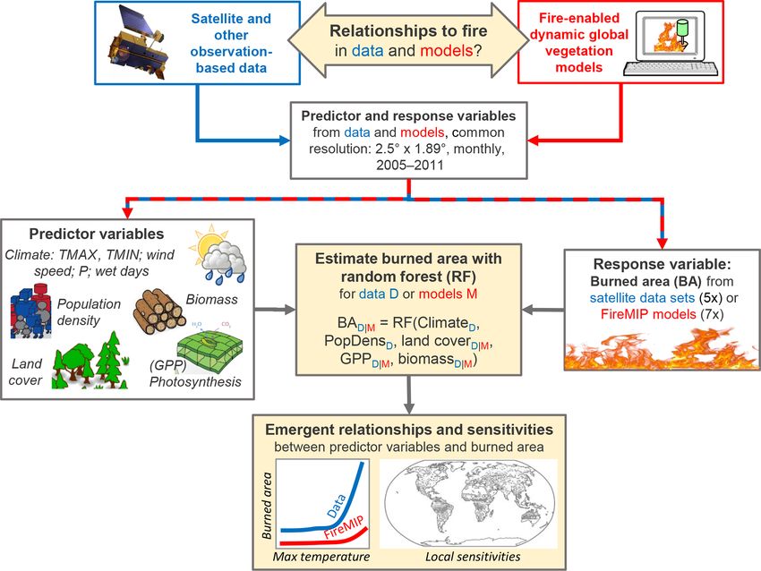
Archibald et al., 2009; Bistinas et al., 2014; Forkel et al., vegetation, and socio-economic predictor variables (Fig. 1).
2017; Krawchuk et al., 2009; Moritz et al., 2012). How- Predictor variables and burned area were either taken from
ever, because of the difficulty of factoring out interactions be- satellite and other observation-based data sets or from simu-
tween predictor variables, such sensitivities represent emer- lations by a suite of fire-enabled DGVMs from the Fire Mod-
gent relationships rather than specific physical controls on eling Intercomparison Project (FireMIP) (Rabin et al., 2017)
fire. Thus, it has proved difficult to disentangle the role of to derive relationships for data sets and models, respectively.
changes in any single factor on the trajectory of changes The RF algorithm is a regression approach that allows
in fire regimes. For example, changes in climate result in non-linear, non-monotonic, and non-additive relations be-
weather conditions that are increasingly favourable for fire tween multiple predictor variables and the target variable.
and fire activity in some temperate regions (Holden et al., RF averages predicted values across an ensemble of decision
Biogeosciences, 16, 57–76, 2019 www.biogeosciences.net/16/57/2019/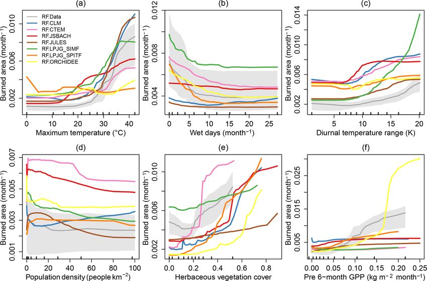
M. Forkel et al.: Emergent relationships with respect to burned area                                                                   59

Figure 1. Overview of the approach for using the random forest machine learning algorithm to derive emergent relationships between several
predictor variables for burned area from satellite and other observation-based data and in fire-enabled DGVMs.

trees that are built based on the training data set (Breiman,          sitivities were derived by computing the individual condi-
2001; Cutler et al., 2012). We built three sets of RF models.          tional expectation (ICE) and the partial dependencies curves
We first built RF models for satellite-observed burned area            (Goldstein et al., 2013). These dependencies represent the
based on a multitude of predictor variables to derive relation-        emergent relationships of burned area to drivers in the
ships from data. There are differences between the available           observation- or model-variable space. We then compared the
burned area data sets; therefore, we used five recent and/or           data- and model-derived emergent relationships and sensitiv-
well-established data sets to encompass these uncertainties.           ities both globally and on a per grid cell basis.
The fire-enabled DGVMs do not use some of the predictor
variables in the satellite-derived RF. Hence, we built a second        2.2   Burned area from satellite data sets
set of satellite-derived RF models with a reduced set of pre-
dictor variables. The third set of RF models was derived for           There are several global burned area data sets; both the spa-
each FireMIP model using the simulated burned area as the              tial patterns and temporal dynamics differ between these
target variable and simulations of gross primary production            models (Hantson et al., 2016; Humber et al., 2018) as they
(averaged over precedent months), biomass and land cover               use different satellite sensors and retrieval algorithms, and
predictor variables, and the population density and climate            have different sensitivities to small fires (Chuvieco et al.,
predictor variables that were used as inputs for the models            2016; Giglio et al., 2013; Randerson et al., 2012). We used
(according to the FireMIP protocol).                                   the variability between five global data sets (Table 1) as an
   From each RF model we then derived the importance                   estimate of uncertainty. However, by doing so we might still
(Sect. 2.7), relationships, and sensitivity (Sect. 2.8) of each        have underestimated the real uncertainty in burned area ob-
predictor variable to burned area. Relationships and sen-              servations because all data sets rely on active fire detec-

www.biogeosciences.net/16/57/2019/                                                                   Biogeosciences, 16, 57–76, 2019
60                                                               M. Forkel et al.: Emergent relationships with respect to burned area

Table 1. Overview of used burned area data sets and FireMIP models.

     Abbreviation       Satellite   data       Spatial resolution and   Satellite        sensor       (all       Reference
     used in this       set or FireMIP         temporal coverage        data      sets      use     thermal
     study              model                                           anomalies               from
                                                                        MODIS)            or       model
                                                                        characteristics.
     Satellite-derived burned area data sets
     GFED4              GFED4                  0.25◦ × 0.25◦            Based       on       MODIS               Giglio et al. (2013)
                                                                        Collection 5 (500 m) (Giglio et al.,
                                                                        2009).
                                               1995–2015
     GFED4s             GFED4s                 0.25◦ × 0.25◦            Based on GFED4 with additional esti-     (Randerson et al., 2012)
                                                                        mation of small fires.
                                               1995–2015
     CCI_MERIS          ESA Fire_cci V4.1      300 m                    MERIS                V4.1                Chuvieco et al. (2016)
                                                                        reflectances.
                                               2005–2011
     CCI_MODIS          ESA Fire_cci V5.0      250 m                    MODIS V5.0.                              Chuvieco et al. (2018)
                                               2000–2015
     MCD64C6            MCD64C6                500 m                    MODIS Collection 6.                      Giglio et al. (2018)
                                               2000–2018
     FireMIP models
     CLM                CLM Li et al. fire     2.5◦ × 1.89◦             Uses WSPEED for fire spread.             Li et al. (2012, 2013)
                        module
                                               1700–2013                Uses PopDens for ignitions and sup-
                                                                        pression.
     CTEM               CTEM                   2.8125◦ × 2.8125◦        Uses WSPEED for fire spread.             Arora and Boer (2005), Melton
                                                                                                                 and Arora (2016)
                                               1700–2013                Uses PopDens for ignitions and sup-
                                                                        pression.
     JSBACH             JSBACH-                1.875◦ × 1.875◦          Uses WSPEED for fire spread.             Lasslop et al. (2014)
                        SPITFIRE
                                               1700–2013                Uses PopDens for ignitions and sup-
                                                                        pression.
     JULES              JULES-INFERNO          1.25◦ × 1.875◦           Empirical model.                         Mangeon et al. (2016)
                                               1700–2013                No WSPEED.
                                                                        Uses PopDens for ignitions only.
     LPJG-SIMF          LPJ-GUESS-             0.5◦ × 0.5◦              Empirical model with seasonal dy-        Knorr et al. (2014, 2016)
                        SIMFIRE-BLAZE                                   namic from GFED3 data set.
                                               1700–2013                No WSPEED for fire spread.
                                                                        Uses PopDens for fire suppression.
     LPJG-SPITF         LPJ-GUESS-             0.5◦ × 0.5◦              Uses WSPEED for fire spread.             Lehsten et al. (2010, 2016)
                        SPITFIRE
                                               1700–2013                Uses PopDens for ignitions.
     ORCHIDEE           ORCHIDEE-              0.5◦ × 0.5◦              Uses WSPEED for fire spread.             Yue et al. (2014, 2015)
                        SPITFIRE
                                               1700–2013                Uses PopDens for ignitions.

tions (thermal anomaly) and reflectance changes from the                      tion from clouds, smoke, snow, and shadows limit burned
same sensor (MODIS). As an exception, CCI_MERIS uses                          area detection. Especially MERIS land observations are sub-
MERIS reflectances combined with MODIS active fires.                          ject to substantial gaps in raw data acquisitions (Tum et al.,
   We restricted our analysis to burned area data with high                   2016). Low observational coverage can result in a strongly
observational quality. Observational quality indicates the de-                underestimated burned area. Here, we used the CCI_MERIS
gree to which missing input satellite imagery or contamina-                   “observed area fraction” layer as a time-variant mask to all

Biogeosciences, 16, 57–76, 2019                                                                            www.biogeosciences.net/16/57/2019/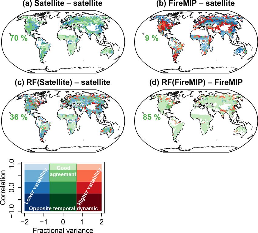
M. Forkel et al.: Emergent relationships with respect to burned area                                                            61

burned area data sets and only included estimates for months       tween −2 and 2 with negative values indicating an underes-
with observational coverage higher than 80 %. We also ex-          timation and positive values indicating an overestimation of
cluded burned area in months with < 0 ◦ C to remove sus-           the observed variance. The reference ref is a vector of the
picious small burned areas in polar regions or in winter           monthly burned area time series from all satellite data sets:
months which are likely caused by insufficiently corrected
gas flares and other industrial activities. Analyses were made     ref = [BA.CCIMERIS , BA.CCIMODIS , BA.GFED4,
with monthly burned area observations for the period from                BA.GFED4s, BA.MCD64C6]
2005 to 2011, which is the common period between the five
data sets.                                                         In the case where a single satellite data set (e.g. x =
                                                                   BA.CCI_MERIS) was compared with the other satellite data
2.3   Burned area from FireMIP models                              sets, this data set was not used in the reference vector. This
                                                                   approach directly considers the differences between data sets
A detailed description of FireMIP DGVMs and the simula-            in the computation of model performance metrics and im-
tion protocol is given by Rabin et al. (2017). Here we used        plies that it is impossible for a FireMIP model or for one
monthly burned area from seven models that made transient          single satellite data set to reach an optimal correlation of
simulations from 1700 to 2013 (bottom half of Table 1). The        unity or a FV of zero as long as the satellite burned area
models were forced using inputs of meteorological variables        data sets show differences. We used the median of the cor-
from the CRUNCEP V5 data set (Wei et al., 2014), monthly           relation coefficient and of the FV for each grid cell to quan-
cloud-to-ground lightning strikes (Rabin et al., 2017), annu-      tify the data–data or model–data agreement over the ensem-
ally updated values of human population density from the           ble of data sets or models. As a single global agreement
HYDE 3.1 data set (Goldewijk et al., 2010), annually updated       metric, we computed the percentage of the land area that
land use and land cover changes from the Hurtt et al. (2011)       showed “good” agreement from the spatial patterns of the
data set, and annually updated values of global atmospheric        Spearman correlation Cor and FV: good agreement for an
CO2 (Le Quéré et al., 2014). Although forcing data sets are        individual grid cell was defined based on a positive and non-
common across DGVMs, they do not use the same set of               random relationship (i.e. Cor ≥ 0.25) and a comparable vari-
forcing variables, i.e. wind speed (WSPEED), or use popula-        ance (−0.75 ≤ FV ≤ 0.75) between simulated and observed
tion density (PopDens) for fire ignitions and/or fire suppres-     burned area.
sion.
   The model outputs were aggregated to a common spa-              2.5     Predictor variables and data sets
tial resolution of 1.89◦ latitude×2.5◦ longitude. Aggregation
was undertaken by averaging the fractional burned area from        Several variables have been identified as predictors of global
all high-resolution grid cells that belong to the same coarse-     fire in previous studies, inter alia the number of dry or wet
resolution grid cell. Nearest neighbour resampling was car-        days per month (WET), diurnal temperature range (DTR),
ried out if less than two high-resolution grid cells were within   maximum temperature (TMAX), grass and shrub cover, leaf
one coarse-resolution grid cell. Analyses were also under-         area index (LAI), net primary production (NPP), popula-
taken for the same period as the common window of the              tion density (PopDens), and gross domestic product (GDP)
satellite data (2005–2011) and by applying the “observed           (Aldersley et al., 2011; Bistinas et al., 2014). Other variables
area mask” from the satellite data.                                have been found important for fire at a regional scale, in-
                                                                   cluding total precipitation, tree cover, forest cover type, tree
2.4   Evaluation of data–data and model–data temporal              height, biomass and litter fuel loads, and grazing (Archibald
      agreement                                                    et al., 2009; Chuvieco et al., 2014; Parisien et al., 2010; Pet-
                                                                   tinari and Chuvieco, 2017). We created a combined set of po-
We evaluated the temporal agreement of monthly burned area         tential variables used in these studies to predict burned area
time series for 2005–2011 between the data sets and between        (Table A1). We used data on gross primary production (GPP)
the data sets and the fire-enabled DGVMs based on various          instead of NPP as GPP can be estimated from eddy covari-
model performance metrics (Janssen and Heuberger, 1995)            ance observations and does not require model assumptions
on a per-grid cell basis. We selected the Spearman rank corre-     about autotrophic respiration.
lation coefficient to compare the temporal agreement and the
fractional variance (FV) to compare the variability of burned      2.5.1    Climate data
area per grid cells:
                                                                   Climate data were taken from the CRUNCEP V5 data set
           σx − σref                                               (Wei et al., 2014). CRUNCEP provides 6-hourly time series
FV =                      ,                                 (1)    of precipitation, maximum and minimum temperature, and
       0.5 × (σx + σref )
                                                                   wind speed. From these time series, we derived the monthly
where σref and σx are the variances of the reference and ob-       mean of daily maximum temperature (CRUNCEP.TMAX)
served or simulated burned area, respectively. FV ranges be-       and minimum temperature (CRUNCEP.TMIN), the monthly

www.biogeosciences.net/16/57/2019/                                                             Biogeosciences, 16, 57–76, 2019
62 M. Forkel et al.: Emergent relationships with respect to burned area
mean daily diurnal temperature range (CRUNCEP.DTR = real forests for the year 2010 (Thurner et al., 2014), and an
TMAX − TMIN), the monthly 90th percentile of daily wind estimate of herbaceous biomass (Carvalhais et al., 2014). The
speed (CRUNCEP.WSPEED), the monthly total precipita- vegetation biomass data set does not cover southern Australia
tion (CRUNCEP.P), and the number of wet days per month or New Zealand. Although fire is common in these regions,
(CRUNCEP.WET). A wet day was defined as a day with we did not fill the global vegetation biomass map with a re-
≥ 0.1 mm precipitation (Harris et al., 2014). gional map to avoid potential artefacts in the derived sensitiv-
ities that would likely result from merging different biomass
2.5.2 Land cover maps. From each FireMIP model, we used the simulated veg-
etation carbon averaged for the years from 2005 to 2011 as
Land cover was taken from the ESA CCI Land cover V2.0.7 the equivalent to this data set. We used canopy height from
data set which provides annual land cover maps for the period Simard et al. (2011); this data set provides a snapshot of
from 1992 to 2015 (Li et al., 2018). Land cover classes were the average canopy height in 2005. Factors related to fuel
converted into the fractional coverage of plant functional properties, specifically grass height, litter depth, woody litter
types (PFTs). For this conversion, we used the cross-walking depth, and the amount of woody litter in different size classes
approach (Poulter et al., 2011, 2015) based on the conversion were extracted from the global fuel bed database (Pettinari
table in Forkel et al. (2017). Individual PFTs combine growth and Chuvieco, 2016). This database is based on a land cover-
form (tree, shrubs, herbaceous vegetation, or crops) with leaf based extrapolation of regional fuel databases for the globe
type (broadleaved or needle-leaved) and leaf longevity (ever- and provides a generic picture of the conditions around 2005.
green or deciduous). The variable Tree.BD, for example, is
the fractional coverage of broadleaved deciduous trees (Ta-
2.5.5 Socio-economic data
ble A1). We created an additional category combining trees
and shrubs (e.g. TreeS.BD = Tree.BD + Shrub.BD) because
most of the FireMIP models simulate woody vegetation We used the annually varying population density data set
rather than separating shrubs and trees explicitly (Table S1 from the HYDE V3.1 database (Klein Goldewijk et al.,
in the Supplement). JULES, LPJG-SIMF, and LPJG-SPITF 2011), which was utilized as a forcing data set for the
dynamically simulate the fractional coverage of PFTs, but FireMIP simulations. We also used annually varying gross
CLM, CTEM, JSBACH, and ORCHIDEE used prescribed domestic product per capita (GDP; World Bank, 2018), a
PFT distributions. We reclassified the PFTs of each model static satellite-derived index of socio-economic development
into the same set of PFTs that we derived from the CCI land based on night-time lights for the year 2006 (Elvidge et al.,
cover data set (Table S1). 2012), and a data set on cattle density for the year 2007 (Wint
and Robinson, 2007).
2.5.3 Vegetation productivity
2.6 Random forest experiments and selection of
Data on gross primary production (GPP) and leaf area index predictor variables
(LAI) were taken to account for the seasonal effects of vege-
tation productivity and canopy development. GPP was taken We performed our analysis using the randomForest pack-
from the FLUXCOM data set which is up-scaled from GPP age V4.6-12 in R (Liaw and Wiener, 2002). We trained the
estimates at FLUXNET measurement sites (Tramontana et RF with 500 regression trees. The training target was either
al., 2016). We used the FLUXCOM data set that used satel- a “satellite-observed” or a “model-simulated” burned area,
lite and CRUNCEP meteorological data for the upscaling. i.e. we trained one RF against each burned area data set and
LAI was taken from MODIS (Myneni et al., 2015). GPP and each individual FireMIP model simulation, respectively. We
LAI were averaged to monthly mean values (e.g. variable used two sets of predictor variables in three sets of RF exper-
name GPP.orig). To account for seasonal fuel accumulation, iments (Table A1):
we also computed previous-season GPP or LAI values as the
mean over the 3 and 6 months before the month of compari-
son with burned area (e.g. GPP.pre3mon and GPP.pre6mon). – “RF.Satellite.full” for satellite-derived RF experiments:
we used 23 of the 28 predictor variables to train RF
2.5.4 Biomass and fuels models for each burned area data set. Five predictor
variables were not included in the RF because they
We used temporally static vegetation data sets to account for were highly correlated with others (r > 0.8, i.e. night-
the effects of vegetation biomass, fuel properties, and ecosys- light development index, cattle density, woody litter for
tem structure on burned area dynamics. Total above- and the 10 h fuel size class, precedent 3-monthly GPP, and
below-ground vegetation biomass was obtained from Carval- precedent 3-monthly LAI; Fig. S1 in the Supplement).
hais et al. (2014), which is based on an above-ground forest The purpose of these experiments was to identify the re-
biomass map for the tropics for the early 2000s (Saatchi et lationship between burned area and each predictor vari-
al., 2011), a total forest biomass map for temperate and bo- able from data sets.
Biogeosciences, 16, 57–76, 2019 www.biogeosciences.net/16/57/2019/M. Forkel et al.: Emergent relationships with respect to burned area 63
– “RF.Satellite.fm” for satellite-derived RF experiments: and one predictor variable for individual cases of the predic-
these experiments were also trained against burned area tor data set (Goldstein et al., 2013). In our application, an in-
data sets but included only the reduced set of 16 data- dividual case is a specific combination of climate, land cover,
based predictor variables that are available from both vegetation, and socio-economic data for a given grid cell in a
observational data sets and the FireMIP (fm) models. given month (Fig. S2). The average of all ICE curves corre-
sponds to the PDP. We used the ICEbox package V1.1.2 for
– “RF.FireMIP.fm” for model-derived RF experiments: R for the computation of ICE curves and partial dependen-
these experiments used the reduced set of predictor vari- cies (Goldstein et al., 2013).
ables with land cover, GPP, biomass, and the response We computed ICE curves for all predictor variables and
variable burned area taken from simulations of each from all RF experiments (Supplement Sects. S4 and S5). We
FireMIP model. The purpose of these experiments was computed ICE curves and PDPs based on the global data set
to compare relationships and sensitivities from satellite- to analyse and compare global emergent relationships. The
and FireMIP-derived RF experiments. Pearson correlation coefficient was computed between pairs
of satellite- and model-derived ICE curves to quantify the
2.7 Importance of predictor variables in random forest
agreement of the emergent relationships (Fig. S15). We also
The normal method of determining the importance of predic- computed PDPs for each grid cell to produce global maps of
tor variables for RFs (increment in the mean-squared error – partial sensitivities for selected predictor variables. To sum-
MSE) was found to be overly sensitive to the burnt area data marize and map the PDP of each grid cell in a single number,
set that was used in training because of the highly skewed we fitted a linear quantile regression to the median between
distribution of burned area, and this hampers its interpretabil- the partial dependence of burned area and the corresponding
ity (Figs. S8, S9). To overcome this issue and to obtain ad- predictor variable and mapped the slope of this regression. In
ditional information about the regional (i.e. grid cell-level) the following, we name this slope “sensitivity”.
importance of predictor variables, we developed an alterna-
tive approach.
This alternative approach uses the fractional variance (FV) 3 Results
and Spearman correlation (r) instead of the MSE and is com-
puted for each grid cell. The importance of variables is quan- 3.1 Evaluation of temporal burned area dynamics
tified as a distance D in a two-dimensional space based on
these metrics: Here we compare the monthly temporal dynamics of burned
q area from the satellite data sets, FireMIP model simulations,
2 2 and random forest predictions for the overlapping period
D = 0.5 × (FVp − FV0 ) + rp − r0 , (2)
from 2005 to 2011. The satellite data sets showed relatively
where FV0 and r0 , and FVp and rp are the performance met- good agreement with each other on average (i.e. “good” is
rics based on the original RF predictions and based on the r ≥ 0.25 and −0.7 ≤ FV ≤ 0.7) over 70 % of the global veg-
RF predictions after permuting a single predictor variable, etated land area, with the best agreement found in frequently
respectively. The FV-related term was multiplied by 0.5 to burning grasslands and savannahs (Fig. 2a). However, indi-
obtain the same range as the correlation. FV and r are com- vidual data sets only showed good agreement over 31 %–
puted at the grid cell-level based on the monthly burned area 56 % of the land area (Fig. S3). The largest dissimilarities
time series from the RF predictions and the training data between burned area data sets occurred in temperate regions
(i.e. burned area from a satellite data set or from a FireMIP with a high land use intensity (e.g. North America, Europe,
model). As the metric D depends on the permutation, we per- China), tropical forests, and in sparsely vegetated arid and
mutated each predictor variable 10 times and averaged the D tundra regions. These difference are likely caused by limited
metric. detection possibilities under cloud cover (e.g. in the Amazon)
and the sensitivities of the algorithms regarding the detection
2.8 Deriving emergent relationships and sensitivities of small fires (temperate and sparsely vegetated regions). As
from random forest the CCI_MERIS data set is based on a different sensor, it is
the most different from the other data sets (31 % of land area
Insight into the shape of a relationship between a predictor showed good agreement, Fig. S3). Hence, these uncertainties
and the target variable in a trained RF can be obtained from make it necessary to separately train RF to each data set in
partial dependence (PDP) (Friedman, 2001) and individual order to assess how such uncertainties translate into emergent
conditional expectation (ICE) plots (Goldstein et al., 2013; relationships to burned area.
Fig. S2). PDPs show the partial relationship between the pre- FireMIP models showed good agreement with satellite
dicted target variable and one predictor variable when other data sets over 9 % of the land area (Fig. 2b). In particu-
predictor variables are set to their mean value. ICE plots lar, models tended to underestimate the variability of burned
show the relationship between the predicted target variable area in key biomass burning regions, while overestimating
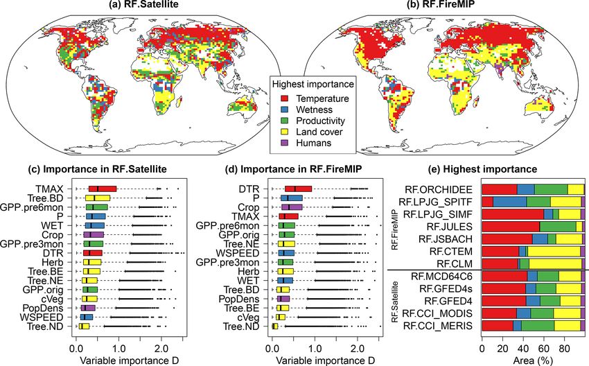
www.biogeosciences.net/16/57/2019/ Biogeosciences, 16, 57–76, 201964 M. Forkel et al.: Emergent relationships with respect to burned area Figure 2. Comparison of temporal burned area dynamics from satellite data sets, fire-enabled DGVMs, and random forest. The maps show the median Spearman rank correlation coefficient and median fractional variance of the monthly burned area from 2005 to 2011 between (a) satellite data sets and the other satellite data sets (Fig. S3), (b) FireMIP model simulations and all satellite data sets (Fig. S4), (c) predicted burned area from RF and all satellite data sets (“full” set of predictor variables, Fig. S5), and (d) predicted burned area from RF trained against FireMIP models and the corresponding simulated burned area from each FireMIP model (Fig. S7). Green percentage numbers indicate the land area with “good” agreement (correlation ≥ 0.25 and −0.7 ≤ FV ≤ 0.7). Regions with missing data (white) either had no vegetation cover (e.g. deserts, ice sheets), had no burned area (e.g. parts of the Amazon and tundra), or were not covered by the vegetation carbon map used (i.e. regions in southern Australia and New Zealand). fire variability in arid and some temperate regions with in- Fig. S7). In summary, the ability of RF models to emulate frequent fire activity. Individual FireMIP models displayed simulated or observed monthly burned area dynamics is suf- weaker performance than the model ensemble (6 % to 8 % ficient for the purposes of comparing satellite-derived and with good agreement, Fig. S4). FireMIP-derived relationships. The RF models can reproduce the temporal dynamics of the satellite burned area data sets reasonably well in most 3.2 Importance of predictor variables in random forest frequently burned regions (Fig. 2c). The overall proportion of the vegetated land area that showed good agreement in Satellite-derived RF experiments show that temperature- “full” experiments was only 36 % but individual RF models related variables were the most important predictors for reached better performances (up to 41 % with good agree- temporal burned area dynamics in temperate and boreal ment, Fig. S5). The “fm” RF models had slightly weaker regions, and land cover- or productivity-related variables performance (22 % to 38 % with good agreement, Fig. S6). were the most important in subtropical and tropical regions However, the performance of RF models was much higher (Fig. 3a). Maximum temperature had on average the high- than the performance of FireMIP models (Fig. 2b). RF est importance globally and was the most important pre- was also able to largely emulate the simulated burned area dictor over 30 %–40 % of the land area in satellite-derived from FireMIP models (85 % with good agreement with the RF (Fig. 3c and e). Productivity and land cover-related vari- FireMIP simulation, Fig. 2d). The RF models most closely ables (i.e. mostly precedent 6-monthly GPP and broadleaved emulated simulated burned area in FireMIP models that deciduous tree cover in savannahs) were the most impor- are based on empirical relationships (JULES, LPJG-SIMF, tant predictors over another 20 %–30 % of the land area. Biogeosciences, 16, 57–76, 2019 www.biogeosciences.net/16/57/2019/
M. Forkel et al.: Emergent relationships with respect to burned area                                                                             65

Figure 3. Grid cell-level importance of predictor variables in satellite- and FireMIP-derived RF experiments. The importance of variables is
quantified as the change in the grid-cell level performance of the RF predictions after a predictor variable is permuted (D metric, see Sect.
2). (a, b) Maps of the group of variables with the highest importance. For example, “temperature” (red) indicates that either TMAX or DTR
had the maximum D metric and were the predictors with the highest importance in a grid cell. Please note that the predicted burned area
in random forest (and in reality) emerges from multiple predictors and that the second-most important predictor (not shown in the maps)
might have similar importance. (c, d) Global distributions of D for each variable from satellite- and model-derived “fm” RF experiments,
respectively. Variables with the same colour are grouped together for the figures in (a), (b), and (e). (e) Area distribution of the variable groups
with the highest D for each RF experiment. In (a) and (b), regions with missing data (white) either had no vegetation cover (e.g. deserts, ice
sheets), had no burned area (e.g. parts of the Amazon and tundra), or were not covered by the vegetation carbon map used (i.e. regions in
southern Australia and New Zealand).

Dryness-related predictor variables (WET and P ) were most                  monthly GPP and showed large differences in the importance
important in tropical forest regions. Human-related predic-                 of land cover-related predictors. The strongly varying size of
tor variables were only most important in a few grid cells,                 the yellow and green bars in Fig. 3e indicate that differences
whereby cropland cover was, on average, of higher impor-                    in simulated burned area between FireMIP models mostly
tance than population density (Fig. 3c). The satellite-derived              originate from how productivity and land cover effects on
importance was very similar among the burned area data sets                 fire are represented.
(Fig. 3e).
   On average, the FireMIP model-derived RF experiments                     3.3     Emergent relationships of burned area to driving
broadly reproduced the satellite-derived importance of pre-                         factors
dictor variables (Fig. 3b). However, maximum temperature,
precedent 6-monthly GPP, and number of wet days had a                       3.3.1    Climate
lower importance, but diurnal temperature range, cropland
cover, and precipitation had a higher importance than in                    The satellite-derived global relationships showed expected
the satellite-derived RFs (Fig. 3d). In addition, the model-                patterns between burned area and climate variables: burned
derived importance of predictor variables differed among                    area increased exponentially with maximum temperature, de-
FireMIP models (Figs. 3e, S10). Most model-derived RF                       creased with an increasing number of wet days per month,
experiments underestimated the importance of precedent 6-                   and increased with diurnal temperature range (Fig. 4a–c).
                                                                            The shapes of the relationships of burned area to climate vari-

www.biogeosciences.net/16/57/2019/                                                                          Biogeosciences, 16, 57–76, 2019
66 M. Forkel et al.: Emergent relationships with respect to burned area Figure 4. Example of global emergent relationships of the fractional burned area per month to predictors from satellite-derived (grey; mean and range based on the five burned area data sets) and FireMIP model-derived (colours) “fm” random forest experiments for six selected variables. Tick marks along the x axis show the deciles (minimum, quantile 0.1 to maximum) of the global distribution of each predictor variable. Maximum temperature was cut at 0 ◦ C in (a) and population density was cut at 100 people km−2 in (d). Emergent relationships for other predictor variables are shown in Figs. S16 and S17. ables were robust among the burned area data sets (Fig. S11). However, burned area data sets show offsets between the relationship curves: for example, the curves that were de- rived from the GFED4s and CCI_MERIS data sets usually show higher burned area than the curves from the other data sets (Fig. S11). These positive offsets are caused by the fact that GFED4s and CCI_MERIS include more small fires and therefore have an overall higher burned area than the other data sets. RF experiments that either use the “full” or “fm” set of predictor variables resulted in largely similar relation- ships (Fig. S12). The relationships between burned area and climate vari- ables were broadly similar for the FireMIP models (Figs. 4a– c, S15, S16). Most model-derived global relationships agreed relatively well (r > 0.5) with satellite-derived relationships for maximum temperature, diurnal temperature range, and the number of wet days (Fig. 5). However, LPJG-SPITF and ORCHIDEE did not reproduce the satellite-derived increase Figure 5. Correlations between global relationships from satellite- of burned area with maximum temperature (Fig. 4a). In the derived and model-derived RF “fm” experiments. Pearson corre- case of LPJG-SPITF, this is likely due to a modification to lations were computed from the relationships as shown in Fig. 4. the calculation of dead fuel moisture. In contrast to other Boxes show the distribution of all model–data correlations (five SPITFIRE implementations, LPJG-SPITF uses soil moisture satellite-derived relationships × seven FireMIP model-derived rela- in part to determine dead fuel moisture. This likely explains tionships). Correlations for individual satellite- and model-derived the failure of LPJG-SPITF to reproduce the dependency on RFs are shown in Fig. S15. maximum temperature and the markedly different behaviour Biogeosciences, 16, 57–76, 2019 www.biogeosciences.net/16/57/2019/
M. Forkel et al.: Emergent relationships with respect to burned area 67
from the other SPITFIRE models seen here. CLM and JS- lation (r = 0.41) to the satellite-derived sensitivity as its in-
BACH did not reproduce the decrease in burned area with ternal formulation reduces burned area with increasing crop-
increasing number of wet days (Fig. 4b). land cover; however, it does not simulate crop fires. These
Regionally, sensitivities to maximum temperature were large differences in the sensitivities of burned area to socio-
positive over most land areas in satellite-derived RF exper- economic variables demonstrate that fire-enabled DGVMs
iments (Figs. 6a, S18). Regional sensitivities to the number mostly disagree on how human effects on fire should be rep-
of wet days were negative over most land areas but were resented.
positive in arid regions and in the boreal regions of north-
ern America (Figs. 6d, S20). Most FireMIP models tended 3.3.3 Land cover, vegetation productivity, and biomass
to overestimate the regional sensitivities between maximum
temperature and burned area in comparison to the satellite- The satellite-derived global relationships to vegetation-
derived sensitivities in most non-forested regions (Fig. 6b–c). related predictor variables showed that burned area increased
Regional sensitivities to wet days were very different among with increasing herbaceous vegetation cover (Fig. 4e), with
FireMIP models and were different to the satellite-derived precedent 6-monthly GPP (Fig. 4f), with precedent 6-
sensitivities (Figs. 6e–f, S21). In summary these results show monthly LAI (Fig. S14b), and with woody litter (Fig. S14h).
that fire-enabled DGVMs broadly reproduced the overall re- The satellite-derived relationships were moderately to highly
lationships and sensitivities of burned area with climate vari- correlated for most land cover types and for vegetation car-
ables. bon (Fig. S15f–o). Regionally, the satellite-derived relation-
ship with herbaceous vegetation cover was positive in most
3.3.2 Socio-economics ecosystems but negative in agricultural areas in Europe, In-
dia, eastern Asia, and North America (Fig. 6j). The regional
The satellite-derived global relationships showed that burned sensitivity to precedent 6-monthly GPP was strongly posi-
area increased exponentially as population density de- tive in most semi-arid regions (Fig. 6m). These relationships
creased at very low values (< 20 people km−2 ) and, gen- reflect the importance of plant productivity and fuel produc-
erally, showed no sensitivity when population density was tion for burned area. Burned area decreased with increas-
> 40 people km−2 (Figs. 4d, S13a). Regionally, the satellite- ing actual-month LAI (Fig. S14a–d), reflecting the fact that
derived sensitivity to population density varied with vege- fires usually do not occur during the wet season when LAI is
tation type. It was negative in most grassland and savan- high in semi-arid regions. Globally, burned area showed a bi-
nah ecosystems but positive in infrequently burned forested modal sensitivity to grass height and litter depth (Fig. S14f–
ecosystems (Fig. 6g). Burned area exponentially increased at g). In summary, the satellite-derived sensitivities demonstrate
a very low gross domestic product per capita (Fig. S13b). The a strong global dependence of burned area dynamics on veg-
relationship between burned area and cropland area was non- etation type and coverage, litter fuels, pre-season plant pro-
monotonic: all data sets showed a burned area peak at < 5 % ductivity, and fuel accumulation.
cropland, minimum burned area at 5 %–30 % cropland cover, FireMIP models reproduced the general increase of burned
and an increasing burned area at > 30 % cropland cover area with increasing herbaceous vegetation (Figs. 4e, 5).
(Fig. S13c). The satellite-derived relationships with cropland However, regional sensitivities to herbaceous cover differed
cover only had moderate correlations with the other satellite- among models (Fig. S25). The satellite-derived increase of
derived relationships for some data sets (e.g. r = 0.53 for burned area with precedent 6-monthly GPP was reproduced
CCI_MODIS, Fig. S15k) because global burned area prod- by LPJG-SPITF, ORCHIDEE, JSBACH, and JULES (r >
ucts are not very accurate for agricultural fires (Hall et al., 0.6) while LPJG-SIMF had a reverse relationship (Fig. 4f).
2016). However, the FireMIP models underestimated the regional
The relationships between burned area and population sensitivity to precedent 6-monthly GPP especially in most
density were very different among FireMIP models and fire-prone semi-arid regions such as African savannahs, Aus-
contrasted somewhat with the satellite-derived relation- tralia, the Mediterranean, and temperate steppes (Fig. 6n–o),
ships (Figs. 4d, S23). ORCHIDEE, LPJG-SIMF, and partly but patterns strongly differed among models (Fig. S27).
CLM and JSBACH reproduced the satellite-derived decline
of burned area with increasing population density (r >
0.4, Fig. S15). LPJG-SPITF, CTEM, and JULES had a 4 Discussion and conclusions
weak agreement with the satellite-derived sensitivities (r <
−0.34). However, the model ensemble median reproduced In summary, fire-enabled DGVMs showed the best correla-
the regionally negative relationships in savannahs and the tions with monthly observed burned area in some savannah
partly positive relationships in forest regions (Fig. 6h–i). regions in Africa and South America. However, models gen-
FireMIP model sensitivities to cropland cover showed large erally underestimated the variance of burned area in most
differences in comparison to satellite-derived sensitivities fire-prone semi-arid ecosystems and overestimated the vari-
(Fig. S16g). Only LPJG-SIMF reached a comparable corre- ance in temperate regions. Using the RF machine learning
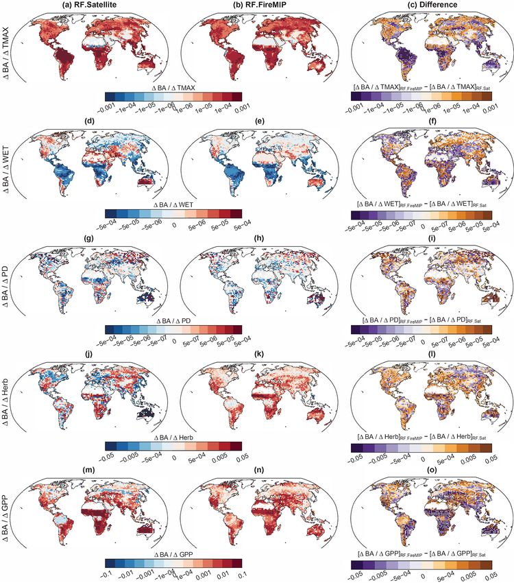
www.biogeosciences.net/16/57/2019/ Biogeosciences, 16, 57–76, 201968 M. Forkel et al.: Emergent relationships with respect to burned area Figure 6. Regional sensitivities of burned area to the driving factors for five selected variables (a–c) maximum temperature, (d–f) number of wet days per month, (g–i) population density, (j–l) herbaceous vegetation cover, and (m–o) precedent 6-monthly GPP. Sensitivities are slopes of a linear quantile regression fit to grid cell-level partial dependencies between burned area and the predictor variables as derived from satellite-derived “fm” RF experiments (left column) and model-derived RF experiments (middle column). The right column shows the difference between model- and satellite-derived sensitivities. Stippling indicates locations where fewer than two model-derived sensitivities are within the range of satellite-derived sensitivities. Sensitivities for individual satellite data sets and FireMIP models are shown in Figs. S18 to S27. Regions with missing data (white) had no vegetation cover (e.g. deserts, ice sheets), had no burned area (e.g. parts of the Amazon and tundra), or were not covered by the vegetation carbon map used (i.e. regions in southern Australia and New Zealand). Biogeosciences, 16, 57–76, 2019 www.biogeosciences.net/16/57/2019/
M. Forkel et al.: Emergent relationships with respect to burned area                                                           69

algorithm, we were able to diagnose reasons for these differ-      the shape of relationships, or the interactions between pre-
ences between data and models: fire-enabled DGVMs largely          dictor variables, unlike algorithms such as generalized addi-
reproduced data-derived relationships and sensitivities be-        tive/linear models (Bistinas et al., 2014; Forkel et al., 2017;
tween burned area and climate variables. However, mod-             Krawchuk et al., 2009). Other flexible algorithms such as
els showed very different relationships with socio-economic        maximum entropy have also been used in empirical fire mod-
variables and generally underestimated sensitivities to pre-       elling (Moritz et al., 2012; Parisien et al., 2016) with very
season plant productivity in all semi-arid ecosystems. As a        similar prediction performance and importance of variables
consequence, these results point towards fuel properties and       compared to random forest (Arpaci et al., 2014). In addition,
fuel dynamics, and human–fire interactions as components of        the emergent relationships between predictors and burned
fire-enabled DGVMs that should be the focus of future model        area that we identified here show the same directions as the
development. In the following, we will discuss methodolog-         relationships that were found in a previous study based on
ical aspects of our applied pattern-oriented model evaluation      generalized linear models (Bistinas et al., 2014). These find-
approach (Sect. 4.1), discuss controls on fire in data and mod-    ings suggest that the choice of machine learning algorithm
els (Sect. 4.2), and finally provide suggestions on how to im-     only marginally affects the direction and overall shape of the
prove fire-enabled DGVMs using current Earth observation           derived relationships.
data sets (Sect. 4.3).
                                                                   4.2   Controls on burned area
4.1   Pattern-oriented evaluation of DGVMs using
      machine learning                                             Following previous studies, we found that climate is the pri-
                                                                   mary control of global burned area which directly affects fire
Simply speaking, simulations of fire (e.g. burned area) in         through weather and fuel moisture conditions, and indirectly
DGVMs can be wrong because (1) the vegetation model                through ecosystem productivity, vegetation type, and fuel
simulates incorrect vegetation distributions, plant productiv-     loads (Archibald et al., 2013; Krawchuk and Moritz, 2011).
ity, and hence fuels, or (2) because the fire module mis-          Fire results from an interplay of several meteorological vari-
represents the response of fire to weather, humans, or fuel        ables, thereby maximum temperature is an important predic-
properties. Classical model benchmarking uses, for exam-           tor globally – especially in northern temperate and boreal
ple, maps of burned area, biomass, and tree cover to quan-         ecosystems. Fire-enabled DGVMs generally reproduced the
tify the model–data mismatch between these variables (Kel-         relationships with maximum temperature but overestimated
ley et al., 2013; Schaphoff et al., 2018). However, classi-        the sensitivity in grassland and savannah ecosystems on av-
cal model benchmarking does not allow one to disentangle           erage. Relationships and sensitivities with the number of wet
the individual effects of the vegetation or fire module on the     days showed larger differences among models and, when
simulated burned area, as errors in the simulated vegetation       compared to satellite-derived relationships, suggest that cli-
might be caused by errors in burned area and vice versa. Be-       mate effects on fuel moisture need to be improved in fire-
cause we use the same climate forcing, and vegetation state        enabled DGVMs.
variables derived from each model in our machine learning             As an indirect climate effect, we found that previous sea-
approach, we are able to evaluate the response of fire mod-        son plant productivity was among the most important predic-
els independent of their underlying DGVMs. This allows us          tor variables globally and was the dominant predictor with
to derive (as partial dependencies or individual conditional       the strongest sensitivity to burned area in semi-arid savan-
expectations) and evaluate the relationships between predic-       nah regions. It has long been recognized that the occurrence
tors and the response for each fire module separately. Hence,      and development of fires is affected by the production and
we are able to attribute deficiencies in fire-enabled DGVMs        accumulation of fuels (Krawchuk and Moritz, 2011; Pausas
to human- and productivity-influences on fire. Previously, a       and Ribeiro, 2013). Plant productivity in fire-prone semi-arid
similar approach also used a tree-based machine learning al-       ecosystems has a high year-to-year variability (Ahlström et
gorithm to evaluate drivers of soil carbon stocks in obser-        al., 2015). Our results demonstrate that the inter-annual vari-
vational databases and in Earth system models (Hashimoto           ability in productivity and hence fuel accumulation is an im-
et al., 2017). Unlike classical model benchmarking, such           portant driver of the variability in burned area. Most fire-
pattern-oriented model evaluation approaches help to diag-         enabled DGVMs poorly captured the importance, relation-
nose the reasons for model–data mismatches.                        ship, and sensitivity of previous-season plant productivity to
   The core of our pattern-oriented model evaluation is the        burned area. This may be a reason why they underestimate
application of a machine learning algorithm to learn emer-         observed variability in burned area and why they misrepre-
gent relationships from data or models. We used the random         sent trends in fire occurrence in Africa as well as globally
forest algorithm because this algorithm has previously been        (Andela et al., 2017).
used to identify drivers of burned area (Aldersley et al., 2011;      While climate and fuel controls when and where fires can
Archibald et al., 2009) and does not require any assump-           burn, humans are responsible for the majority of fire igni-
tions about the statistical distribution of predictor variables,   tions while also simultaneously suppressing fire. We found a

www.biogeosciences.net/16/57/2019/                                                             Biogeosciences, 16, 57–76, 2019
70 M. Forkel et al.: Emergent relationships with respect to burned area
strong decline of burned area with increasing population den- loads exist (van Leeuwen et al., 2014) and global maps of
sity between 0 and 20 people km−2 which confirms previous fuel properties are based on spatial extrapolations including
findings (Bistinas et al., 2014; Knorr et al., 2014). Human various assumptions and uncertainties (Pettinari and Chu-
effects on fire emerge from various activities such as tradi- vieco, 2016). As an alternative, hybrid data–model-based ap-
tional land use practices (shifting cultivation, hunting, graz- proaches such as land carbon cycle data assimilation systems
ing, and grassland burning), the use of fires for land clear- (Bloom et al., 2016) may provide consistent information to
ing or as tool in land conflicts, from prescribed small fires benchmark vegetation productivity, turnover, and litter fuel
within fire management, and from unintended or illegal ig- dynamics in DGVMs.
nitions (Archibald, 2016; Bowman et al., 2011; Lauk and Fire largely depends on the vegetation type (Rogers et al.,
Erb, 2009; van Marle et al., 2017). The modest performance 2015). Also our results show consistent land cover-specific
of random forest regarding reproducing satellite burned area relationships to burned area in satellite data, but these rela-
suggests that we did not capture the complexity of human– tionships differ among FireMIP models and in comparison
fire interactions with the set of predictor variables used. For to the satellite-derived relationships (Fig. S17). Vegetation
example, the complex non-monotonic relationship between types and associated morphological, biochemical, and struc-
burned area and cropland cover suggests that agricultural tural characteristics of plants affect the flammability and fire
land use has diverging effects on fire in different agricul- tolerance of vegetation (Archibald et al., 2018; Pausas et al.,
tural regions of the world (Fig. S13c) (Korontzi et al., 2006). 2017). Although global fire models have PFT-specific param-
However, alternative variables such as cattle density or the eterizations for flammability (Thonicke et al., 2010), such
night light-based index of socio-economic development were fire-relevant plant characteristics need to be incorporated in
highly correlated with population density or cropland cover DGVMs (Zylstra et al., 2016). Such efforts should be com-
at the coarse resolution of our analysis; therefore, they did plemented by calibrating DGVMs against satellite observa-
not add to prediction performance of random forest. At re- tions that provide relevant information about the spatial dis-
gional scales, land use or infrastructure-related variables are tributions of fuel structure (Pettinari and Chuvieco, 2016; Ri-
important predictors for fire (Archibald et al., 2009; Arpaci et año et al., 2002), fuel moisture content (Yebra et al., 2013,
al., 2014; Chuvieco and Justice, 2010; Parisien et al., 2010). 2018), fire ignitions and spread (Laurent et al., 2018), fuel
However, these regional findings also show that the impor- consumption (Andela et al., 2016), and fire radiative energy
tance of human-related predictors largely differs between re- (Kaiser et al., 2012). In summary, besides human–fire inter-
gions, which complicates its applicability for global-scale actions, we identified vegetation effects on fire as a main de-
fire modelling. However, random forest largely emulated the ficiency of fire-enabled dynamic global vegetation models in
simulated burned area from FireMIP models, which suggests simulating temporal dynamics of burned area.
that we indeed included the main predictors for the model
world. Although some newer global fire models include the
effects of cropland and pasture management on fires (Ra- Code availability. This analysis is based on R (version 3.3.2) us-
bin et al., 2018), the complexity of human–fire interactions ing the randomForest (version 4.6-12) and ICEbox (version 1.1.2)
currently lacks a solid and large-scale empirical basis that packages. R and previously mentioned packages are available from
would allow researchers to derive alternative formulations on the Comprehensive R Archive Network (CRAN, https://CRAN.
R-project.org/package=randomForest (Breiman and Cutler, 2018);
human–fire interactions for fire-enabled DGVMs.
ICEbox, https://CRAN.R-project.org/package=ICEbox (Goldstein
et al., 2017), last access: 9 January 2019).
4.3 Improving vegetation controls on fire in DGVMs
Our results demonstrate that the role of vegetation on fire Data availability. Data are available from the references as indi-
needs to be better represented in fire-enabled DGVMs to ac- cated in Table A1.
curately simulate the variability of burned area. The links be-
tween vegetation productivity, fuel production, and fire need
to be improved. Fuel production depends on plant productiv-
ity, and on the allocation, turnover, and respiration processes
of carbon in different fuel types. As a first step for model im-
provement, fire-enabled DGVMs need to be tested and pos-
sibly re-calibrated against observations or observation-based
estimates of plant productivity, above-ground biomass, and
carbon turnover (Carvalhais et al., 2014; Thurner et al., 2016,
2017). Beyond total above-ground biomass, the evaluation of
different fuel types (e.g. biomass in wood, canopy and un-
derstory, and litter size classes) is currently hampered by the
availability of data. Only a few in situ measurements of fuel
Biogeosciences, 16, 57–76, 2019 www.biogeosciences.net/16/57/2019/You can also read