Intercomparison of freshwater fluxes over ocean and investigations into water budget closure - HESS
←
→
Page content transcription
If your browser does not render page correctly, please read the page content below
Hydrol. Earth Syst. Sci., 25, 121–146, 2021
https://doi.org/10.5194/hess-25-121-2021
© Author(s) 2021. This work is distributed under
the Creative Commons Attribution 4.0 License.

Intercomparison of freshwater fluxes over ocean
and investigations into water budget closure
Marloes Gutenstein1 , Karsten Fennig1 , Marc Schröder1 , Tim Trent2 , Stephan Bakan3 , J. Brent Roberts4 , and
Franklin R. Robertson4
1 DeutscherWetterdienst, Offenbach, Germany
2 EarthObservation Science, University of Leicester, Leicester, UK
3 Max Planck Institute for Meteorology, Hamburg, Germany
4 NASA Marshall Space Flight Center, Huntsville, AL, USA

Correspondence: Marloes Gutenstein (marloes.gutenstein@dwd.de)

Received: 24 June 2020 – Discussion started: 30 July 2020
Revised: 6 November 2020 – Accepted: 20 November 2020 – Published: 7 January 2021

Abstract. The development of algorithms for the retrieval of      nity to investigate the consistency between E and P data sets.
water cycle components from satellite data – such as total        Over ocean, P (nearly) balances with E if the net transport
column water vapor content (TCWV), precipitation (P ), la-        of water vapor from ocean to land (approximated by over-
tent heat flux, and evaporation (E) – has seen much progress      ocean VIMD, i.e., ∇ · (vq)ocean ) is taken into account. On a
in the past 3 decades. In the present study, we compare six re-   monthly timescale, linear regression of Eocean − ∇ · (vq)ocean
cent satellite-based retrieval algorithms and ERA5 (the Euro-     with Pocean yields R 2 = 0.86 for ERA5, but smaller R 2 val-
pean Centre for Medium-Range Weather Forecasts’ fifth re-         ues are found for satellite data sets.
analysis) freshwater flux (E − P ) data regarding global and         Global yearly climatological totals of water cycle compo-
regional, seasonal and interannual variation to assess the de-    nents (E, P , E −P , and net transport from ocean to land and
gree of correspondence among them. The compared data sets         vice versa) calculated from the data sets used in this study
are recent, freely available, and documented climate data         are in agreement with previous studies, with ERA5 E and P
records (CDRs), developed with a focus on stability and ho-       occupying the upper part of the range. Over ocean, both the
mogeneity of the time series, as opposed to instantaneous ac-     spread among satellite-based E and the difference between
curacy.                                                           two satellite-based P data sets are greater than E − P , and
   One main finding of our study is the agreement of global       these remain the largest sources of uncertainty within the ob-
ocean means of all E − P data sets within the uncertainty         served global water budget.
ranges of satellite-based data. Regionally, however, signifi-        We conclude that, for a better understanding of the global
cant differences are found among the satellite data and with      water budget, the quality of E and P data sets needs to be
ERA5. Regression analyses of regional monthly means of E,         improved, and the uncertainties more rigorously quantified.
P , and E − P against the statistical median of the satellite
data ensemble (SEM) show that, despite substantial differ-
ences in global E patterns, deviations among E − P data are
dominated by differences in P throughout the globe. E − P         1   Introduction
differences among data sets are spatially inhomogeneous.
   We observe that for ERA5 long-term global E − P is very        The water and energy cycles are key components of Earth’s
close to 0 mm d−1 and that there is good agreement between        climate system. Energy exchange from water phase changes
land and ocean mean E − P , vertically integrated moisture        plays a direct role in atmospheric heating; therefore, precip-
flux divergence (VIMD), and global TCWV tendency. The             itation (P ) and evaporation (E) are two critical processes
fact that E and P are balanced globally provides an opportu-      connecting the land–ocean surface and overlying atmosphere
                                                                  (Trenberth et al., 2009). The difference between E and P

Published by Copernicus Publications on behalf of the European Geosciences Union.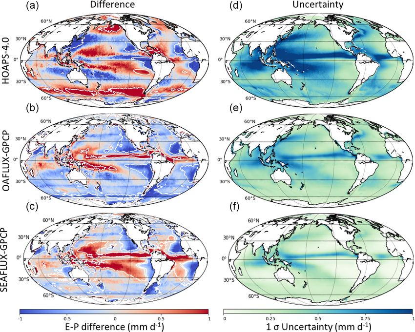
122                                                                        M. Gutenstein et al.: Freshwater fluxes over ocean

rates, E − P , is the freshwater flux from the surface to the at-   of these data sets, all freely available climate data records
mosphere, which is positive where E dominates and negative          (CDRs), characterized by the stability of input data and re-
where P dominates. Over the global oceans, total E − P is           trieval algorithms, emphasizing data homogeneity over local,
positive, as a considerable amount of water evaporates from         instantaneous accuracy. European Centre for Medium-Range
the oceans and is transported to land by advection, mainly          Weather Forecasts (ECMWF) ERA5 reanalysis data (Hers-
in the form of water vapor, where it precipitates. Averaged         bach et al., 2020) are included for comparison in the present
over a year, changes in atmospheric storage vanish, and net         study. Our main focus lies with the assessment of correspon-
negative E − P over land is balanced by continental runoff          dence among E − P data sets on a global and regional scale
of water into the ocean. Although numerous studies have ad-         by the intercomparison of six data sets and putting the re-
dressed the question of how variations in the ocean state af-       sults into perspective regarding uncertainty estimates. More-
fect the water cycle and freshwater fluxes with a particular        over, we investigate to what extent water budget closure is
view on global warming (Wentz et al., 2007; Trenberth et al.,       achieved by satellite-based over-ocean estimates by compar-
2007; Schlosser and Houser, 2007; Robertson et al., 2014),          ing with ERA5 data and previously published estimates of
a clear and consistent picture has yet to emerge – one of the       water cycle components.
significant challenges in climate science (Bony et al., 2015;          Here, we consider the atmospheric water vapor budget
Hegerl et al., 2014; Allan et al., 2020).                           with a focus on the oceans, where satellite observations of
   At long temporal and/or large spatial scales, the increases      E are available. The net change in atmospheric water vapor
in E and P with rising global temperature are relatively            content can be written as
small (2–3 % K−1 ) and are constrained by the energy budget.        δW
At smaller scales (less than approximately 4000 km and/or               = E − P − ∇ · (vq),                                     (1)
                                                                     δt
10 years) these changes can be much larger (or smaller) due
to dynamical contributions (Dagan et al., 2019; Yin and Por-        with W being the total column water vapor and ∇ · (vq) the
porato, 2019; Allan et al., 2020). The nature and extent of         moisture flux divergence, i.e., the amount of moisture re-
these changes, which affect the livelihoods of many millions        moved by dynamical transport from the considered volume.
of people, are difficult to model due to various counteracting      See Table 2 for all symbols and abbreviations. Compared to
influences such as forcing by clouds and aerosols, or land use      water vapor, the contributions of liquid water and ice are very
change (Allan et al., 2020). Close monitoring of E and P by         small (e.g., Berrisford et al., 2011) and can be safely ignored
(satellite) observations thus yields an important contribution      in the context of this study.
to a better understanding of impacts of climate change at re-          On a global scale ∇ ·(vq) vanishes (as the Earth is a closed
gional and local scales.                                            system), and Eq. (1) reduces to
   The study of the global water cycle is not only compelling
from a scientific point of view: it also aids the evaluation        1W = E − P ,                                                (2)
of climate models and reanalyses by verifying the degree
                                                                    where, for brevity, we write the W tendency during large
of consistency among the various components of the cycle.
                                                                    (monthly) time steps as 1W .
Such an approach is adopted here for the evaluation of satel-
                                                                       Assuming that 1W is small compared to E and P , Eq. (2)
lite observations of E and P , which, particularly over ocean,
                                                                    dictates that global total E must equal global total P . Hence,
are difficult to validate otherwise. The fact that the global
                                                                    an observed imbalance in global totals of E and P indi-
water cycle is closed puts a strong constraint on global to-
                                                                    cates either an inconsistency in E and P data sets or a
tal E and P fluxes. This has been exploited in various stud-
                                                                    change in the global water cycle, for example an increase
ies in the past (Trenberth et al., 2007, 2011; Schlosser and
                                                                    in the amount of atmospheric water vapor (possibly caused
Houser, 2007; Berrisford et al., 2011; Trenberth and Asrar,
                                                                    by global warming), invalidating the assumption that 1W is
2014; Trenberth and Fasullo, 2013; Seager and Henderson,
                                                                    negligible. Moreover, globally, E and P covary, meaning that
2013; Robertson et al., 2014) from which the general con-
                                                                    their interannual, seasonal, and even monthly variability are
clusion emerged that, although much progress has been made
                                                                    correlated.
regarding E and P estimates, observations and models still
                                                                       At regional scales and for monthly averages, 1W is small
require substantial improvements in accuracy to achieve bud-
                                                                    compared to E − P and ∇ · (vq), so that Eq. (1) can be ap-
get closure.
                                                                    proximated by
   Over the years, methods to determine E and P based
(mainly) on satellite data have been developed and repeat-          E − P = ∇ · (vq).                                           (3)
edly updated: HOAPS E and P (Andersson et al., 2017),
J-OFURO E (Tomita et al., 2019), IFREMER E (Bentamy                 This is particularly valid for the large ocean and land regions,
et al., 2013), SEAFLUX E (Roberts et al., 2020), OAFlux             and, since globally ∇ · (vq) = 0, from Eq. (3) it follows that
E (Yu et al., 2008), and GPCP P (GPCP, 2018) are among
the most widely used data sets. Acronyms are explained in           (E − P )ocean = ∇ · (vq)ocean = −∇ · (vq)land
Sect. 2 and listed in Table 1. We present an intercomparison                      = −(E − P )land ,                             (4)

Hydrol. Earth Syst. Sci., 25, 121–146, 2021                                           https://doi.org/10.5194/hess-25-121-2021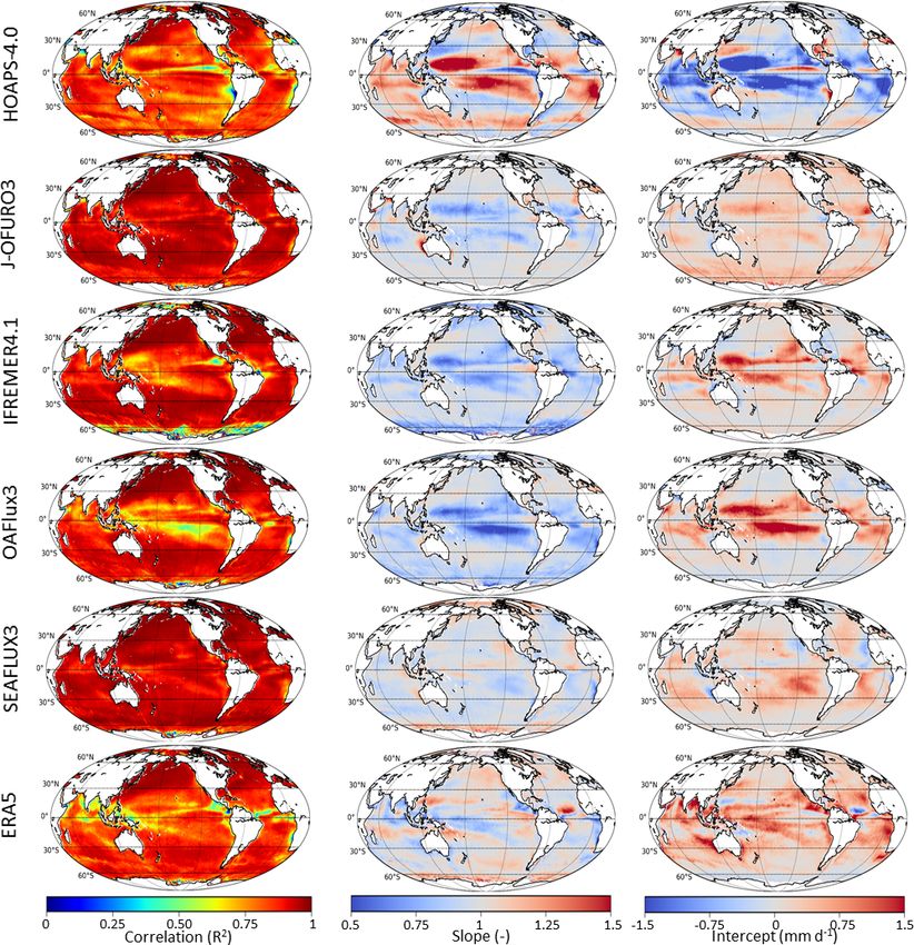
M. Gutenstein et al.: Freshwater fluxes over ocean                                                                                                                  123

Table 1. Compilation of the data sets used within this study. Most data sets contain more variables than those listed here.

  Acronym                 Data set name                                        Date range               Resolution      Variables           Reference
  ERA5                    ECMWF Reanalysis 5                                   Jan 1979 to present      0.25◦ × 0.25◦   E, P , TCWV, VIMD   Hersbach et al. (2020)
  GPCP-1DD V 1.3          Global Precipitation Climate Program                 Jan 1996–Dec 2017        1.0◦ × 1.0◦     P                   Huffman et al. (2001)
  HOAPS V4.0              Hamburg Ocean Atmosphere Parameters                  Jul 1987–Dec 2014        0.5◦ × 0.5◦     E, P , E − P        Andersson et al. (2010)
                          and Fluxes from Satellite
  J-OFURO V3              Japanese Ocean Flux Data Sets with Use of            Jan 1988–Dec 2013        0.25◦ × 0.25◦   LHF, E − P          Tomita et al. (2018)
                          Remote-Sensing Observations
  OAFlux                  Objectively Analyzed Air-sea Fluxesa                 1958–2019 (monthly)      1.0◦ × 1.0◦     E                   Yu et al. (2008)
  V3                                                                           1985–2017 (daily)
  IFREMER V4.1            Institut Français de recherche pour                  Jan 1992–Dec 2018        0.25◦ × 0.25◦   LHF, SST            Bentamy et al. (2013)
                          l’exploitation de la mer
  SEAFLUX V3              Sea Flux Project                                     Jan 1988–Dec 2018        0.25◦ × 0.25◦   LHF, SST            Roberts et al. (2020)

∗ ftp://ftp.whoi.edu/pub/science/oaflux/data_v3 (last access: January 2021).

Table 2. Abbreviations and symbols of variables used throughout                              spatial averages, as random errors (no covariance) disap-
the paper.                                                                                   pear for large numbers of data points, whereas systematic
                                                                                             errors (100 % covariance) do not. When there is a lack of in-
  Variable                                              Abbreviation      Symbol             formation on error covariances, OAFlux3 and SEAFLUX3
  Air density                                           –                 ρ                  monthly mean uncertainty estimates are similarly treated to
  Evaporation rate                                      E                 E                  having 100 % covariance. An estimate of uncertainty is pro-
  Latent heat flux                                      LHF               Ql
  Near-surface (10 m) humidity                          –                 qa
                                                                                             vided with ERA5 data in the form of results from a 10-
  Near-surface (10 m) wind speed                        –                 u                  member ensemble (Hersbach et al., 2020).
  Precipitation rate                                    P                 P                     In the following section, we provide some background on
  Runoff                                                R                 R                  E and P retrievals and introduce the E, P , and other data
  Sea surface humidity                                  –                 qs
  Sea surface temperature                               SST               Ts                 sets used for our study. Section 3 details the methods applied
  Latent heat of evaporation of water                   –                 LE                 to the various data sets to enable a fair comparison. Results of
  Total column water vapor                              TCWV              W                  our analyses are presented and discussed in Sects. 4–5, and
  TCWV tendency                                         1TCWV             1W
                                                                                             we close our study with a set of conclusions and recommen-
  Turbulent exchange coefficient                        –                 CE
  Vertically integrated moisture flux divergence        VIMD              ∇ · (vq)           dations.

                                                                                             2       Data sets
with subscripts denoting summation over ocean or land. This
separation into land and ocean contributions allows us to as-                                In this intercomparison study, we assess the degree of
sess the consistency of different E and P data sets, as satellite                            agreement between five satellite-based E retrievals, two
E data are not available over land.                                                          observation-based P retrievals, and a reanalysis data set. In
   In addition to the spatiotemporal distributions of indi-                                  this section, the retrieval algorithms will be briefly intro-
vidual budget terms, for example E − P , information on                                      duced: for more details, please refer to the literature listed
the accuracy and precision of that value is of importance.                                   in Table 1.
Uncertainty estimates indicate whether observed differences                                     The retrieval of E from satellite observations is challeng-
– between data sets (e.g., observations and models), over                                    ing. It is determined from the bulk flux parameters near-
time (trends, variability), or in space – are statistically rel-                             surface wind speed and humidity gradient near the surface.
evant. Moreover, they play a major role in data assimilation.                                Wind speed can be retrieved from satellite passive microwave
Quantification of retrieval uncertainty, however, is a difficult                             brightness temperature (BT) measurements, and BTs have
task, particularly for nonlinear retrieval algorithms such as                                also some sensitivity to near-surface specific humidity. Spe-
those used to retrieve E and P from satellite observations.                                  cific humidity at the ocean surface is derived from sea sur-
Of the E CDRs investigated here, HOAPS-4.0, OAFlux3,                                         face temperature (SST). All satellite-based E algorithms use
and SEAFLUX3 provide monthly mean uncertainty ranges.                                        reanalysis data to some extent, and, vice versa, ERA5 also
In HOAPS, random and systematic uncertainty components                                       assimilates satellite data. Hence, these products cannot be
are provided separately (Kinzel et al., 2016), allowing error                                considered completely independent, and the distinction be-
propagation along with the calculation of temporal and/or                                    tween “satellite data” and “reanalysis” is somewhat artificial

https://doi.org/10.5194/hess-25-121-2021                                                                         Hydrol. Earth Syst. Sci., 25, 121–146, 2021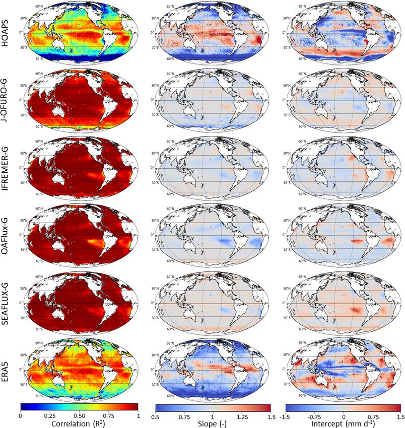
124                                                                       M. Gutenstein et al.: Freshwater fluxes over ocean

and not always appropriate. However, for historical reasons       stable fundamental climate data records (see, e.g., Wentz
– and for lack of a suitable alternative – we will retain these   et al., 2013; Sapiano et al., 2013; Berg et al., 2018; Fennig
terms throughout this paper.                                      et al., 2020), which then serve as input to various satellite re-
   The main characteristics of the evaporation retrieval from     trievals. Slight differences in calibration approaches lead to
passive microwave data are common to all satellite algo-          differences in FCDRs that propagate into the retrieved data.
rithms, but there is quite some variation regarding the input     Issues with sensor stability, especially with SSM/I and SS-
of Level 1 (calibrated observations) and Level 2 (retrieval re-   MIS sensors, usually express themselves as slow drifts or
sults) data, as will be discussed below. First, we will give a    sudden jumps of the global mean.
brief description of the retrieval basics, followed by details
of the various satellite algorithms.                              2.1.1   HOAPS-4.0

2.1   Evaporation data records                                    HOAPS (Andersson et al., 2010) relies almost completely on
                                                                  satellite data, as it only uses an ERA-Interim profile clima-
The liquid-water-equivalent evaporation rate, E, is calculated    tology as a priori starting point for the 1D-Var retrieval of u
from the latent heat flux Ql as follows:                          and the humidity profile (Graw et al., 2017). The only other
      Ql                                                          auxiliary data set is the daily Optimum Interpolated Sea Sur-
E=       ,                                                 (5)    face Temperature (OISST; Reynolds et al., 2007), version 2,
      LE
                                                                  derived from AVHRR satellite data. OISST provides SST at
where LE is latent heat of evaporation of water. The latent       a depth of 0.5 m which is transformed to a skin SST using the
heat flux, in turn, is parameterized according to the bulk flux   approach by Donlon et al. (2002), which is then used for the
algorithm (based on the Monin–Obukhov similarity theory           determination of qs . The parameterization described in Ben-
representation of fluxes in terms of mean quantities):            tamy et al. (2003) is used to determine qa . For calculation
                                                                  of the flux parameters Ql and E, HOAPS-4.0 uses COARE
Ql = ρLE CE u(qs − qa ),                                   (6)    version 2.6a (Bradley et al., 2000), which is nearly identical
                                                                  to COARE-3.0 (Fairall et al., 2003). HOAPS-4.0 is a CDR
with being ρ the density of air; CE the coefficient of tur-
                                                                  derived from the CM SAF (Climate Monitoring Satellite Ap-
bulent exchange; u the wind speed at 10 m height relative
                                                                  plication Facility) BT FCDR (Fennig et al., 2017, 2020)
to the ocean surface current speed; and qs and qa the spe-
                                                                  and is available at 0.5◦ and 6-hourly (except E − P ) and
cific humidity at the sea surface and at 10 m height, respec-
                                                                  monthly resolution from July 1987 to December 2014 (An-
tively. Whereas qa and u are derived from satellite obser-
                                                                  dersson et al., 2017). HOAPS data can be obtained from
vations of BT, ρ, qs , and LE are derived from their depen-
                                                                  https://wui.cmsaf.eu (last access: January 2021).
dences on SST and/or air temperature. The turbulent ex-
change coefficient CE is obtained from the Coupled Ocean-
Atmosphere Response Experiment (COARE) version 3.0 al-            2.1.2   J-OFURO3
gorithm (Fairall et al., 1996, 2003). The algorithm iteratively
                                                                  The latest update to J-OFURO involved improvements in the
estimates stability-dependent scaling parameters and wind
                                                                  methods of flux retrieval and expansion of the data set in
gustiness to account for sub-scale variability.
                                                                  terms of time range and parameters (Tomita et al., 2019). The
   Most of the data sets used here do not explicitly contain E;
                                                                  algorithm is similar to that described above. In addition to
therefore, we calculated those from monthly means of Ql and
                                                                  BT from SSM/I and SSMIS (from Remote Sensing Systems
SST using Eq. (5) and LE (in J kg−1 ) given by (Henderson-
                                                                  (RSS), Wentz et al., 2013), J-OFURO3 uses BT data from
Sellers, 1984)
                                                                  AMSR-E and AMSR2 (JAXA Version 3 and 2.1, respec-
                                      2                         tively), and TMI (1B11 Version 7 from NASA–GES DISC)
                     6          Ts
LE = 1.91846 × 10 ×                       ,                 (7)   for the retrieval of flux parameters. To determine qa , a pa-
                            Ts − 33.91
                                                                  rameterization based on BTs, total column water vapor, and
where Ts is SST in kelvin. The slight difference with the def-    water vapor scale height was developed using match-ups of
inition of LE used in the COARE-3.0 algorithm causes neg-         in situ buoy- and ship-based qa and DMSP-F13 BTs from
ligible differences of 0.03–0.04 % for Ts between 278 and         eight channels (Tomita et al., 2018). From the instantaneous
298 K.                                                            qa values, gridded daily averages are determined and inter-
   The BT observations common to satellite-based retrievals       calibrated to DMSP-F13 qa to remove systematic differences
of ocean turbulent fluxes come from the Special Microwave         caused by the use of different FCDRs. The Ts required for
Imager (SSM/I; Hollinger et al., 1990) and Special Mi-            the calculation of qs and other flux parameters is the me-
crowave Imager/Sounder (SSMIS; Liman et al., 2008) in-            dian value of an ensemble of 12 in situ, satellite-based, and
struments on the Defense Meteorological Satellite Program         reanalysis data sets. Other auxiliary data sets include water
(DMSP) platforms F08–F18. These data were corrected and           vapor surface mixing ratios from ERA-Interim (Dee et al.,
intercalibrated using various approaches to create FCDRs,         2011), OSTIA sea ice concentration (Donlon et al., 2012),

Hydrol. Earth Syst. Sci., 25, 121–146, 2021                                         https://doi.org/10.5194/hess-25-121-2021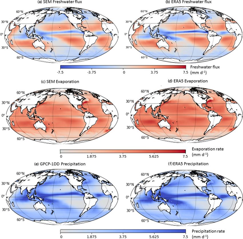
M. Gutenstein et al.: Freshwater fluxes over ocean                                                                          125

and air temperature from NCEP–DOE reanalysis (Kanamitsu           mission Level 1C intercalibrated BTs (Berg et al., 2018). Fol-
et al., 2002). Near-surface wind speed is determined as the       lowing the results of Roberts et al. (2019), the retrieval al-
simple mean of values derived from microwave radiometers          gorithms now include additional a priori information on the
and scatterometers (Tomita et al., 2019). J-OFURO3 is avail-      vertical stratification of water vapor and lower-tropospheric
able at 0.25◦ and daily resolution from 1988 to 2013. It was      stability. A total of 14 passive microwave imagers – includ-
acquired from https://j-ofuro.scc.u-tokai.ac.jp/ (last access:    ing SSM/I, SSMIS, TMI, AMSR-E, AMSR-2, and GMI – are
January 2021).                                                    used for satellite retrievals, and double differences are used
                                                                  to intercalibrate all estimates to the GPM GMI radiometer.
2.1.3   OAFlux3                                                   The satellite retrievals are made in clear and cloudy scenes
                                                                  but are screened for precipitating conditions. A Kalman
Satellite data used for the production of OAFlux3 data            smoother is then applied to the retrieved estimates to blend
include wind speed from active (scatterometer) and pas-           the MERRA-2 (Modern-Era Retrospective analysis for Re-
sive (radiometer) microwave instruments, SST from OISST           search and Applications, Version 2; Gelaro et al., 2017) back-
(Reynolds et al., 2007), and qa from the Goddard Satellite-       ground with satellite observations in an hourly gap-free anal-
Based Surface Turbulent Fluxes Dataset Version 2 and 2c           ysis. A diurnally varying sea surface skin temperature from
(GSSTF2.0; Chou et al., 2003; Shie et al., 2009). These are       the SEAFLUX CDR (Clayson and Brown, 2016) is used to-
merged with NCEP and ERA40 reanalysis data using weight-          gether with the near-surface meteorology to estimate fluxes
ing factors that put more emphasis on satellite data (for u) or   using the COARE 3.5 algorithm (Edson et al., 2013). Uncer-
on reanalyses (qa ), or weights both equally (Ts ) whenever       tainties are estimated for the individual near-surface mete-
satellite data are available (Yu et al., 2008). OAFlux3 data      orology as a blending of the retrieval and background errors
are available from 1958 to 2018 (monthly) or 1985 to 2017         through application of the Kalman smoother. Estimates of the
(daily) at 1◦ resolution from ftp://ftp.whoi.edu/pub/science/     surface flux uncertainties are computed using standard prop-
oaflux/data_v3 (last access: January 2021).                       agation of error techniques through the bulk flux algorithm.
2.1.4   IFREMER4.1
                                                                  2.1.6   ERA5
Similar to J-OFURO and OAFlux, IFREMER’s ocean flux
retrieval algorithm is based on a synergy of remote sens-         ERA5 is the current operational reanalysis running at
ing and reanalysis data (Bentamy et al., 2013). The cur-          ECMWF, the European Centre for Medium-Range Weather
rent version 4.1 contains, among other things, latent heat        Forecasts. Compared to its predecessor, ERA-Interim, ERA5
flux (LHF) and SST at daily and monthly, 0.25◦ resolution         includes improved model physics, improved data assimila-
from 1992 to 2018. The BTs used for retrievals are intercal-      tion techniques, and higher spatial (31 km) and temporal (1 h)
ibrated by Colorado State University (CSU; Sapiano et al.,        resolution. These lead to a gain in forecasting skill of up
2013), except for data beyond June 2017, where CSU data           to 1 d compared to ERA-Interim (Hersbach et al., 2020).
end and a switch to BTs from RSS (Wentz et al., 2013)             Among many other observations, ERA5 assimilates the CM
is made. Intercalibrated scatterometer wind data (Bentamy         SAF BT FCDR (Fennig et al., 2017); conditions for SST
et al., 2017a) are supplemented by wind speeds determined         are prescribed using HadISST2.1 (Kennedy et al., 2016) and
by RSS from the SSM/I, SSMIS, and WindSat instruments.            OSTIA (Donlon et al., 2012) from September 2007 onwards
SST are from OISST (Reynolds et al., 2007). The model re-         (Hersbach et al., 2020). ERA5 encompasses data from 10 re-
lating BTs to qa using satellite–in situ data match-ups was       analysis runs at a reduced spatial resolution of 62 km, al-
updated from Bentamy et al. (2003) and now includes two           lowing estimation of the uncertainty range from ensemble
additional terms: Ts and Ta − Ts (with Ta the air temper-         statistics. The analysis presented here is performed with the
ature at 10 m height from interpolated ERA-Interim data;          ECMWF ensemble mean, whereas uncertainty is determined
Bentamy et al., 2013). IFREMER4.1 data were obtained via          from the ensemble. Both data sets were interpolated to 1◦
https://wwz.ifremer.fr/oceanheatflux/Data (last access: Jan-      resolution at ECMWF.
uary 2021).                                                          The monthly averaged data set, available from the Coper-
                                                                  nicus Climate Data Store (https://cds.climate.copernicus.eu/,
2.1.5   SEAFLUX3                                                  last access: January 2021), contains, among many other
                                                                  things, total column water vapor (TCWV), vertically inte-
The SEAFLUX3 data set consists of the near-surface mete-          grated moisture flux divergence (VIMD), total precipitation,
orology and surface turbulent fluxes of heat, moisture, and       and evaporation rates (ECMWF, 2019). Monthly averages
momentum for the period 1988–2018 at an hourly, 25 km             are calculated from daily means starting at 00:00 UTC and
resolution (Roberts et al., 2020). An extension of the Roberts    ending at 00:00 UTC the following day (ECMWF, 2020).
et al. (2010) neural network retrieval has been developed to      Evaporation rates are derived from the gradients of specific
estimate near-surface wind speed, humidity, and air temper-       humidity between the surface and the lowest model level
atures from the Global Precipitation Measurement (GPM)            (10 m for ERA5) as described above (ECMWF, 2016). The

https://doi.org/10.5194/hess-25-121-2021                                         Hydrol. Earth Syst. Sci., 25, 121–146, 2021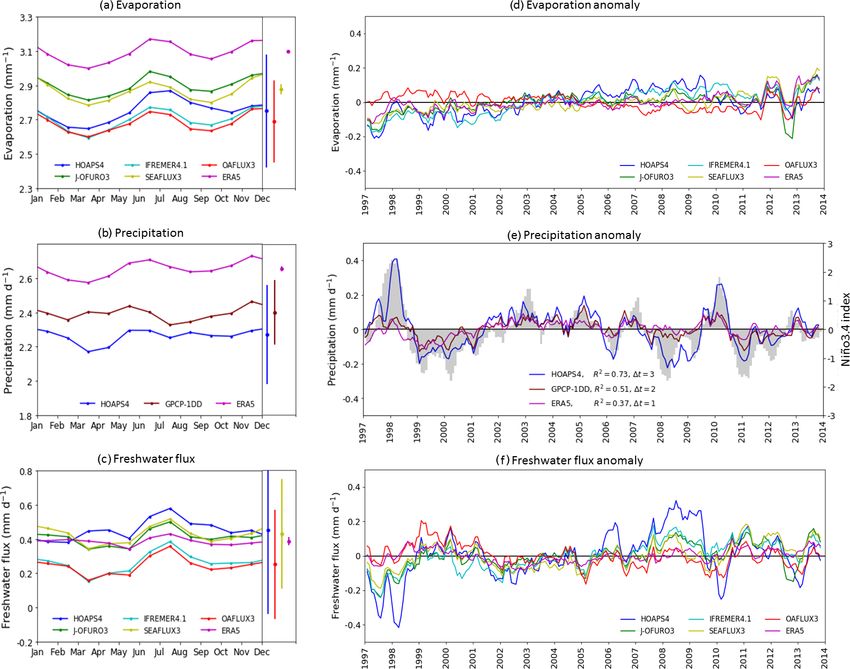
126                                                                     M. Gutenstein et al.: Freshwater fluxes over ocean

main differences between the satellite-based retrievals de-      ing biases of HOAPS Level 2 E with respect to collocated in
scribed here and ERA5 determination of E are the consis-         situ ship-based data into equally populated E, u, Ts , and W
tency of atmospheric variables involved (u, qa , qs ) and the    bins. The mean and standard deviation of the biases are as-
high temporal sampling rate: monthly means are determined        sumed to represent the systematic and random components
from (daily means of) hourly data from forecasts initial-        of the 2σ uncertainty range, respectively, which is probably
ized daily at 06:00 and 18:00 UTC. Moreover, satellite-based     a conservative estimate. When the approach is taken of de-
data sets only provide fluxes over ocean, whereas ERA5           termining uncertainty ranges as a function of turbulent flux
contains data over land and ocean. VIMD – i.e., the total        parameters, these can also be assigned to times and regions
amount of water vapor removed from the atmospheric col-          not covered by the ship-based reference data set (Liepert and
umn by dynamical transport – is provided in ERA5 as a grid-      Previdi, 2012). For the current study, we calculated the mean
ded monthly mean field. We calculated the TCWV tendency          uncertainty by averaging the systematic uncertainty compo-
in month x from monthly mean ERA5 data by subtracting            nent. The random component is negligible when averaging
TCWV of month x + 1 from TCWV of month x − 1, then               long time series. The HOAPS P data set does not contain
dividing by 30 d per month to obtain the mean TCWV ten-          uncertainty information; instead, a constant relative 1σ un-
dency in km3 d−1 . This was converted to units of mm d−1 by      certainty range of 13 % was assumed, based on a comparison
multiplication with the Earth’s surface area for comparison      with ship-based in situ data (Burdanowitz, 2017). The total
with freshwater fluxes.                                          E − P uncertainty was determined by error propagation.
                                                                    Bias errors given in the OAFlux data set were computed
2.2   Precipitation data records                                 based on the uncertainty ranges of individual input data sets,
                                                                 assuming no correlation between uncertainties from differ-
Microwave-based retrievals of precipitation are based on         ent data sets (Yu et al., 2008). Like for HOAPS uncertainty
the interaction of liquid or solid hydrometeors with the up-     ranges, the OAFlux bias error was simply averaged for our
welling radiation field. In HOAPS-4.0, P is determined by        investigations.
a neural network retrieval trained on profiles from an ERA-         Uncertainties in SEAFLUX arise both from comparisons
Interim climatology (Andersson et al., 2010). The training       of the individual retrieval errors (e.g., wind speed, humidity,
data set consists of 1 month (August 2004) of assimilated        air temperature) evaluated against quality-controlled buoy
SSM/I BTs and the corresponding ERA-Interim P (Bauer             archives and from errors arising as a result of gap-filling
et al., 2006).                                                   through application of a Kalman smoother. Individual re-
   There are a multitude of global precipitation products in     trievals were generally found to be unbiased globally, but
existence (see, e.g., Kidd and Huffman, 2011; Tapiador           some conditional biases likely remain. The total uncer-
et al., 2017), but for this study we selected GPCP as the P      tainty is a measure of the reduction in retrieval uncertainties
data set with which to calculate E−P (except for the HOAPS       through combination of multiple sensors at each location and
product, which makes use of its own P data) because it is        time and increases in uncertainty related to sampling inho-
generally regarded as the data set that performs best glob-      mogeneities. As the length of time grows between any given
ally. Moreover, J-OFURO also makes use of GPCP P to de-          time and the previous or next observation, the sampling un-
termine E − P (Tomita et al., 2019).                             certainty increases. Thus the SEAFLUX uncertainties gener-
   The Global Precipitation Climatology Project–One-             ally capture random retrieval uncertainties and sampling un-
Degree Daily data set (GPCP-1DD; denoted GPCP here-              certainty but do not contain conditional systematic errors as
after) contains P estimated from a combination of data from      developed for HOAPS. However, we note that the retrieval
ground-based rain gauges and satellites – the latter including   error itself does likely contain some components of condi-
near-infrared, passive, and active microwave observations        tional systematic biases even though the unconditional biases
(Huffman et al., 2001). Daily global precipitation rates are     remain small.
provided by GPCP-1DD at 1◦ resolution for the time range            In contrast to the monthly GPCP product, GPCP-1DD
1996–2017. We calculate monthly mean P from version 1.3          Version 1.3 does not provide explicit uncertainty estimates;
GPCP-1DD (GPCP, 2018), because the spatial resolution of         hence here we assume a constant relative 1σ uncertainty
the monthly product is not sufficient for our purposes. These    range of 8 %. This is the estimated bias error for GPCP data
data were obtained from https://rda.ucar.edu/datasets/ds728.     over the tropical oceans (Adler et al., 2012), which is where
5/ (last access: January 2021).                                  most of the P signal originates. Over the global oceans, the
                                                                 bias error was estimated at 10 %, but Adler et al. (2012) con-
2.3   Errors, biases, and uncertainty                            sidered this an upper bound.
                                                                    In contrast to uncertainty ranges estimated by comparing
Four out of seven data sets analyzed here contain explicit in-   with other (e.g., in situ) data sets, the uncertainty of ERA5
formation on uncertainty. HOAPS contains estimates of ran-       data is described by the standard deviation and the range
dom and systematic bias errors (Kinzel et al., 2016; Liepert     of the ensemble, consisting of 10 separate reanalysis runs
and Previdi, 2012). The errors in E were obtained by separat-    (Hersbach et al., 2020). We determined these statistics after

Hydrol. Earth Syst. Sci., 25, 121–146, 2021                                        https://doi.org/10.5194/hess-25-121-2021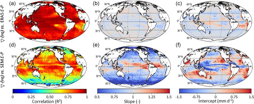
M. Gutenstein et al.: Freshwater fluxes over ocean                                                                             127

averaging of the data: first, the mean (e.g., global monthly       (510 × 106 , 350 × 106 , or 160 × 106 km2 , respectively). Sea-
mean) of each individual ensemble member was calculated,           sonally varying numbers of observations screened out due
and then standard deviation and range were determined. Note        to sea ice are neglected. Most comparisons in this study are
that ERA5 ensemble statistics should be interpreted in a rela-     shown in area-specific units, but for the comparison of global
tive sense (i.e., ensemble spread is larger where uncertainty is   totals over land and ocean presented in Sect. 4.6, data were
higher), as the numerical values are overconfident (ECMWF,         converted to area-integrated units (km3 yr−1 ) so that the to-
2020).                                                             tals balance.
                                                                      Global total runoff from ERA5 and other data sets was
                                                                   determined by calculating the area integral of all points.
3   Methods

HOAPS is the only satellite data set containing E, P , and         4     Results
E − P data from a single source (i.e., microwave BTs).
Within the HOAPS algorithm, E −P is obtained by subtract-          4.1    Freshwater flux climatology
ing monthly mean P from E (Andersson et al., 2010). For
this study, the data were remapped from 0.5 to 1◦ . For the        Freshwater flux climatologies obtained from 17 years of data
J-OFURO3 freshwater flux product, monthly mean GPCP-               (1997–2013) were determined from satellite ensemble me-
1DD P is subtracted from the corresponding J-OFURO E               dian (SEM) and ERA5 data. They are shown in Fig. 1a and
(Tomita et al., 2019). We determined E − P of the other            b, to illustrate the overall spatial distribution of mean E − P .
satellite-based data sets by subtracting monthly mean GPCP         The chosen time range is the largest common time range of
P from the respective monthly mean E. These data sets will         the data sets used in this study. Note that ERA5 data were
be denoted as IFREMER-G, SEAFLUX-G, and OAFlux-                    matched to satellite data coverage.
G to indicate that GPCP data were subtracted. J-OFURO,                Regions where mean P > E are dominated by atmo-
IFREMER, and SEAFLUX do not provide E; therefore we                spheric freshwater outflux (into the ocean), appear in blue in
calculated those from their respective LHF and SST data us-        Fig. 1a and b, and are concentrated at the Intertropical Con-
ing Eqs. (5) and (7). The calculation of E from Ql was per-        vergence Zone (ITCZ) and the Pacific warm pool. In the sub-
formed at 0.5◦ and monthly resolution. Applying the same           tropics, E generally outweighs P . At higher latitudes P and
method of calculating E from HOAPS monthly mean LHF                E are approximately equal, but with a tendency to E−P < 0.
and SST data causes negligible differences with monthly            Comparison of panels c–f with a and b shows that the E − P
mean E determined from instantaneous LHF and SST data              pattern is mainly determined by P in the tropical and high-
(root mean square differences of ≤ 0.01 mm d−1 for individ-        latitude regions but determined by E in the subtropical re-
ual grid boxes during 1997–2013). All E data were conser-          gions. The agreement between SEM and ERA5 E − P cli-
vatively remapped to 1◦ to match GPCP resolution prior to          matologies is good, yet some systematic differences can be
subtraction of P . Similarly, ERA5 E − P was determined by         observed. Due to higher P in the ITCZ, ERA5 shows more
subtracting monthly mean P from E at 1◦ resolution.                negative E − P there. Conversely, the overall higher E level
   All comparisons presented here are performed with col-          in ERA5 causes E − P values larger than those found for
located data; i.e., only grid boxes (at x, y, and t) present       SEM over most of the global oceans. Excessive E was also
in all data sets were used to create climatological or global      found to produce high E − P in ERA-Interim (Brown and
averages. A more accurate collocation procedure would be           Kummerow, 2014).
performed at shorter, for example daily, timescale, because           The deviations are more apparent when climatological dif-
differences in filtering of high-precipitation scenes (where E     ferences are analyzed. For this comparison we select ERA5
retrieval is impaired) and selection of included satellite in-     as a reference due to its spatiotemporal completeness and
struments lead to differences in sub-monthly sampling. This        because it is the only “other” data set (i.e., not satellite
was, however, not feasible in this study, as HOAPS and J-          data), keeping in mind that ERA5 data very likely also
OFURO E −P data are only provided at monthly resolution.           have inaccuracies and/or biases. Figure 2 shows climato-
   The satellite reference data set used in regional compar-       logical difference plots of HOAPS (upper panel), OAFlux-
isons is determined by the statistical median of the satellite-    G (middle panel), and SEAFLUX-G (lower panel) with
based data ensemble and therefore does not include ERA5.           collocated ERA5 data. Although HOAPS differences with
The median is chosen over the mean to exclude outliers.            ERA5 appear larger to the eye, root mean squared differ-
In the following, this reference data set is abbreviated SEM       ences are 0.6 mm d−1 for each of the three comparisons:
(satellite ensemble median).                                       0.60 mm d−1 for HOAPS, 0.58 mm d−1 for SEAFLUX-G,
   Global averages were determined by converting the area-         and 0.57 mm d−1 for OAFlux-G. As already seen in Fig. 1,
specific unit of mm d−1 (equivalent to kg m−2 d−1 ) to units       differences are not homogeneously distributed over the
of km3 d−1 ; computing the global, ocean, or land mean;            globe. The HOAPS difference plot is characterized by an al-
and multiplying with the corresponding total surface area          ternating pattern of positive and negative deviations. Stronger

https://doi.org/10.5194/hess-25-121-2021                                           Hydrol. Earth Syst. Sci., 25, 121–146, 2021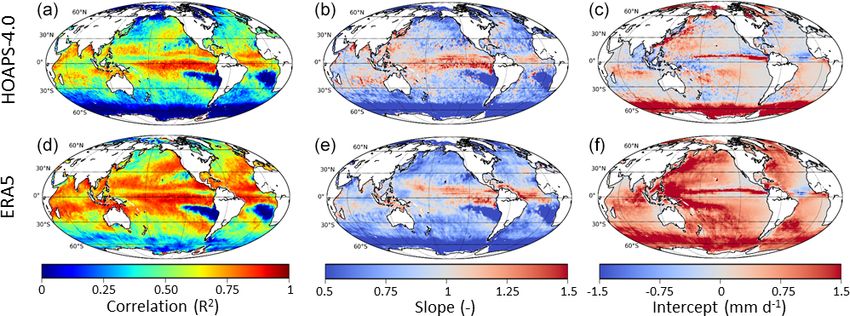
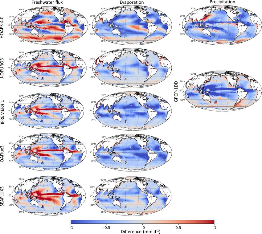
128                                                                           M. Gutenstein et al.: Freshwater fluxes over ocean

Figure 1. Satellite ensemble median (SEM) and ERA5 climatologies (1997–2013) of freshwater flux (a, b) and evaporation (c, d), and GPCP
and ERA5 precipitation (e, f). ERA5 data coverage was reduced to match satellite data, and data over land were discarded from panels (e)
and (f). See the text for details.

HOAPS E in the subtropical central north and eastern South            Atlantic Ocean, except in the upwelling regions on the west
Pacific produces elevated E − P compared to ERA5. In con-             coasts of Africa and the Americas. The difference plots of
trast, elevated ERA5 E over the East China Sea combines               J-OFURO and IFREMER-G with ERA5 are not shown here
with smaller ERA5 P in the region, resulting in higher ERA5           but are very similar to the lower left panel because the dif-
E − P . The positive bands on either side of the Equator are          ferences in P between GPCP and ERA5 are larger than dif-
due to higher HOAPS E, whereas the negative E − P dif-                ferences in E in most regions. All plots, including difference
ferences at the Equator are due to smaller HOAPS P . The              climatologies of E and P , can be found in the Appendix,
negative deviations to the east and west of Australia are             Fig. A1.
also due to differences in P , whereas the deviations at lat-            To investigate where the differences are significant, the
itudes > 40◦ S are due in equal parts to E and P . The dif-           right column of Fig. 2 presents the 1σ uncertainty range
ferences between OAFlux-G and ERA5 are mainly due to                  from HOAPS (upper panel), OAFlux-G (middle panel), and
P , apart from the regions in the subtropical Pacific and At-         SEAFLUX-G (lower panel). Moreover, regions where the
lantic Oceans, where OAFlux E is smaller than ERA5 E.                 difference between satellite E−P and ERA5 E−P is greater
SEAFLUX-G shows slightly larger differences with ERA5.                than the 2σ uncertainty range are enclosed by white con-
In the band within 30◦ of the Equator, SEAFLUX yields                 tour lines in the left panels. The ERA5 E − P uncertainty
higher E than ERA5 (and OAFlux) in most of the Pacific and            shows a pattern similar to that of OAFlux-G but is a factor of

Hydrol. Earth Syst. Sci., 25, 121–146, 2021                                              https://doi.org/10.5194/hess-25-121-2021
M. Gutenstein et al.: Freshwater fluxes over ocean                                                                        129

Figure 2. Difference maps of HOAPS (a), OAFlux-G (b), and SEAFLUX-G (c) climatological mean E − P minus the corresponding
collocated ERA5 climatology (1997–2013). HOAPS (d), OAFlux-G (e), and SEAFLUX-G (f) climatological mean 1σ uncertainty. White
lines in the left panels enclose regions where the difference with ERA5 E − P exceeds the 2σ uncertainty range.

10 smaller than the uncertainties estimated for satellite data   cles were determined for the overlapping time range (1997–
and therefore adds a negligible component to the total uncer-    2013) and are shown in Fig. 3a–c. HOAPS, ERA5, OAFlux,
tainty estimate. The HOAPS uncertainty range is larger than      SEAFLUX, and GPCP uncertainty ranges are presented in
HOAPS-ERA5 E − P differences over most of the globe.             the boxes attached to the right of panels a–c. Dots show the
This is mainly due to P , for which we assumed 13 % un-          climatological mean value, and error bars indicate the asso-
certainty. The deviations > 1 mm d−1 in the oceans’ desert       ciated 1σ uncertainty. Subtracting the seasonal cycle from
regions (off the west coasts of Peru and southern Africa) and    the respective monthly mean time series yields global ocean
in the higher latitudes are clearly outside the 2σ uncertainty   anomalies of E − P , E, and P , which are presented as 3-
ranges. In contrast, OAFlux-G E − P deviations are larger        month running means in panels d–f. Seasonal and interan-
than the estimated 2σ uncertainties in the ITCZ, on the west     nual variability are on the same order of magnitude, which
coasts of the Pacific and Atlantic Ocean, in the Arabian Sea,    can be seen by comparing the left panels with those on the
and at southern high latitudes. Again, the uncertainty range     right (the y axis spans 1 mm d−1 in all panels).
is mainly given by P , for which we assumed a relative un-          There are substantial deviations between E, P , and E − P
certainty of 8 %. Due to the small uncertainty estimates in      data. Fig. 3a shows that a difference of about 0.2 mm d−1
SEAFLUX, all of the larger differences with ERA5 in the          is found between OAFlux and J-OFURO E. An additional
Atlantic and Pacific Ocean are significant.                      discrepancy of 0.2 mm d−1 exists between J-OFURO and
                                                                 ERA5. E data from HOAPS, IFREMER, and OAFlux are
4.2   Intercomparison of freshwater flux over ocean:             much closer to each other: satellite-based E all falls within
      global means                                               the OAFlux uncertainty range (red error bars), whereas the
                                                                 ERA5 climatological mean E does not fall within the larger
Monthly mean E, P , and E − P of six (or three) data             HOAPS uncertainty range. The HOAPS uncertainty range is
sets were collocated (see Sect. 3) and averaged over the         much larger than the seasonal variation, which indicates that
global oceans (80◦ S–80◦ N). Climatological seasonal cy-

https://doi.org/10.5194/hess-25-121-2021                                        Hydrol. Earth Syst. Sci., 25, 121–146, 2021
130 M. Gutenstein et al.: Freshwater fluxes over ocean
Figure 3. Climatological (1997–2013) seasonal cycle of global ocean mean evaporation rate (a), precipitation rate (b), and freshwater flux (c).
HOAPS, ERA5, OAFlux, SEAFLUX, and GPCP mean values and associated 1σ uncertainty ranges are shown in the boxes to the right of the
panels. Monthly mean anomaly (with respect to the climatological seasonal cycle depicted on the left) over the global oceans (80◦ S–80◦ N)
of evaporation rate (d), precipitation rate (e), and freshwater flux (f). The anomaly data are smoothed using a 3-month running mean. Panel
(e) additionally displays the Niño3.4 index shifted by +3 months (right y axis). The legend shows the correlation coefficient of the Niño3.4
index with P anomalies and the time lag of highest correlation (1t in months). Ticks on the time axis mark January of the indicated year.
it is likely overestimated, which may be due to the assump- comparison of E − P (not specific E or P algorithm issues),
tion of 100 % covariance for systematic uncertainty. we only describe the observed differences between P (and
Fig. 3b shows that the seasonal cycle of global ocean E) data sets to obtain a better understanding of differences
mean P is shallow, and the two satellite-based data sets agree between E − P data.
within the GPCP uncertainty for 10 months of the year. Like Apart from HOAPS E − P in March–April, all satellite
for E, we find substantial differences among the three P data sets agree on phase and amplitude of the E −P seasonal
data sets: there is a deviation of about −0.1 mm d−1 between cycle (Fig. 3c). ERA5 shows hardly any dependence on sea-
HOAPS and GPCP, and ERA5 shows values that are about son, as the magnitude of the summer maximum is smaller in
0.25 mm d−1 higher than GPCP, which was also found by ERA5 due to the relatively larger summer P maximum. The
Hersbach et al. (2020). These differences can, in part, be ex- monthly and interannual variability of ERA5 E − P is, like
plained by differences in P frequency distributions and, in the seasonal cycle, of smaller amplitude than that of satel-
particular, by the fraction of rain occurrences, which is much lite data, which is caused by the high degree of coherence
lower in HOAPS than in GPCP or ERA5. This will be dis- between E and P , and will be discussed in more detail in
cussed in Sect. 5. Since in this paper the focus is on the inter- Sect. 4.5. Because, compared to satellite data, ERA5 E and
Hydrol. Earth Syst. Sci., 25, 121–146, 2021 https://doi.org/10.5194/hess-25-121-2021M. Gutenstein et al.: Freshwater fluxes over ocean 131
P are biased high by about the same amount, E − P is close correlation with SEM is found for J-OFURO and SEAFLUX,
to the satellite data. HOAPS yields the highest E − P due with R 2 exceeding 0.75 essentially everywhere.
to its low mean P . All E − P data are contained within the The middle panels of Fig. 4 display the slope of the lin-
HOAPS and OAFlux uncertainty ranges. ear regression. A slope greater (smaller) than 1 implies an
The E anomalies in Fig. 3d display a high degree of cor- overestimation (underestimation), particularly of large val-
relation on a monthly timescale. On a multi-annual scale ues, compared to SEM. HOAPS overestimates E in the trop-
all data sets show some degree of variability, which is ics, except in an area in the eastern Pacific at 0–5◦ N, where
most likely linked to sensor and intercalibration issues (e.g., a < 1. J-OFURO, IFREMER, and OAFlux each yield slopes
Robertson et al., 2020), and the variability is not consistent. < 1 within 30◦ of the Equator and slopes close to 1 every-
For example, the slow, decadal-scale oscillation observed in where else (apart from the band with a < 1 seen in IFRE-
HOAPS and IFREMER appears to be in anti-phase compared MER at high southern latitudes). Of those three E data sets,
to OAFlux. The three P data sets yield interannual variations OAFlux displays the largest deviations from a = 1. In con-
with amplitudes that are similar in amplitude to those found trast, SEAFLUX yields slopes close to unity over the whole
for E and show a high degree of correspondence in their globe. An inhomogeneous pattern is found for ERA5, but the
monthly and interannual variability – apart from the stronger slope is generally close to 1. A small region in the tropical
dependence of HOAPS on ENSO (El Niño–Southern Oscil- Atlantic stands out due to its large slope, and since this is not
lation) phase. This is a known characteristic of HOAPS data seen in any of the satellite data sets, it must be a feature in
(see, e.g., Andersson et al., 2011; Masunaga et al., 2019) and ERA5 data.
is most apparent in panel e, where the Niño 3.4 SST index The patterns in the middle panels are nearly all mirrored
(Trenberth and Stepaniak, 2001) is plotted in gray bars along in the right panels; i.e., wherever large values are overesti-
with P anomalies: HOAPS P correlates with Niño 3.4 if a mated (a > 1), small values are underestimated (b < 0), and
lag of 3 months is taken into account (R 2 = 0.73). Appar- vice versa. All data sets thus appear to agree on intermedi-
ent agreement is found among all E − P anomalies (panel ate values. Overall, the correspondence between E data sets
f) – again apart from the ENSO-related deviations found in is best in the subtropics, while the largest deviations appear
HOAPS P . The agreement among E − P anomalies is best mainly in the tropics. This is due to the frequent occurrence
in the “quiet” ENSO years (2001–2005), but this is proba- of weather conditions in which the moisture stratification de-
bly a coincidence as the spread in E − P in other years is parts substantially from typical conditions to which the re-
mainly due to differences in E and not in P . Note that dif- trieval algorithms of near-surface moisture are tuned. Ac-
ferences between J-OFURO-G, IFREMER-G, SEAFLUX- counting for this dependence on moisture stratification, as
G, and OAFlux-G are due to differences in E, as in all cases in the SEAFLUX and J-OFURO algorithms, improves re-
GPCP P was used for the calculation of E − P . trieval results appreciably compared to in situ measurements
(Roberts et al., 2019).
4.3 Intercomparison of freshwater flux over ocean: Figure 5 shows the same analysis for P from HOAPS (up-
time series on regional scales per panels) and ERA5 (lower panels). The correlation coef-
ficient between HOAPS and GPCP P is > 0.75 in the ITCZ
In this section, we investigate the temporal correlation of wa- and about 0.5 for most of the global oceans. In the oceans’
ter cycle components on regional scales. This approach will deserts R 2 < 0.25 is found, which is mostly due to the small
help to elucidate differences between the various data sets by dynamic range of mean P . Compared to GPCP, HOAPS un-
uncovering in which regions the differences are particularly derestimates P in this region, as a < 1. At latitudes pole-
large (or small). As a reference for the E and E − P compar- ward of 50◦ similarly small R 2 values are found that are due
isons, we use SEM, a data set determined by the statistical in part to the small dynamic range and in part to difficulties
median of all satellite data sets. Since we use only two satel- pertaining to the detection of snow by passive microwave in-
lite P data sets, GPCP is selected as a reference for the P struments (Tapiador et al., 2017; Kidd and Huffman, 2011).
comparison. We determine correlation coefficient, slope, and HOAPS underestimates high P here and overestimates small
intercept of the linear regression (y = ax+b) between 1◦ ×1◦ P (b > 0 mm d−1 ) compared to GPCP. Very similar patterns
monthly means (not anomalies) of each data set, y, and the are seen for ERA5, although in general the correlation co-
reference, x, to examine where estimates are most consistent. efficient is higher than for HOAPS. ERA5 is biased high
The results are shown for all six E data sets in Fig. 4, almost everywhere compared to GPCP. Both HOAPS and
where the left column displays the correlation coefficient. In ERA5 show a smaller range of P in the Southern Oceans,
the top row, HOAPS yields R 2 > 0.75 over most of the globe, as the slope is less than 0.5, but the large intercept indicates
with some notable exceptions in the ITCZ and at the Peruvian an overestimation of small P compared to GPCP. The narrow
coast. The other satellite data yield higher correlation coeffi- band of R 2 < 0.75 and b > 1 mm d−1 at the Equator is also
cients. The correlation pattern of ERA5 with SEM is similar found in both HOAPS and ERA5.
to that found for HOAPS, although the tropical areas with For E −P , the results of the regression analysis are shown
R 2 < 0.75 are not at the same locations. The highest overall in Fig. 6. The highest correlation coefficients (and slopes and
https://doi.org/10.5194/hess-25-121-2021 Hydrol. Earth Syst. Sci., 25, 121–146, 2021132 M. Gutenstein et al.: Freshwater fluxes over ocean Figure 4. Correlation, slope, and intercept of the linear regression of monthly mean E from (top to bottom) HOAPS, J-OFURO, IFREMER, OAFlux, SEAFLUX, and ERA5 with satellite ensemble median (SEM) monthly mean E (1997–2013). intercepts closest to 1 and 0 mm d−1 ) are found among the for E−P than for P . In summary, the correlation patterns for data sets calculated with GPCP P . This shows that most of HOAPS and ERA5 indicate agreement on the seasonal cycle the variability in E − P is due to differences in P . Since in the tropics, a result found previously by Brown and Kum- GPCP P is used in four out of five data sets included in merow (2014), although we find that its amplitude is reduced the SEM, those data sets show high correlations, whereas in the GPCP-based E − P data (Fig. 3). Less agreement is HOAPS and ERA5 yield patterns very similar to those found found in the Southern Oceans, where GPCP-based E − P is for the P comparison in Fig. 5. Nevertheless, both for ERA5 underestimated relative to SEM. At the midlatitudes, the re- and HOAPS the correlation in most of the tropics is higher gression with SEM yields slopes near 1 and intercepts close Hydrol. Earth Syst. Sci., 25, 121–146, 2021 https://doi.org/10.5194/hess-25-121-2021
M. Gutenstein et al.: Freshwater fluxes over ocean 133
Figure 5. Correlation, slope, and intercept of the linear regression of monthly mean P from HOAPS (a–c) and ERA5 (d–f) with GPCP
monthly mean P (1997–2013).
to 0 mm d−1 for ERA5 and HOAPS, but the correlation is over ocean; the error bars on the over-land E − P are smaller
less than in the tropics, probably due to the smaller dynamic than the graph’s line width. This is due in equal parts to E
range of E − P . and P , which have similar ensemble standard deviations (not
In the present study, we compare satellite-based E − P shown). For the time range shown in Fig. 7 global E − P is
with ERA5 E − P because we are also examining the sep- seen to oscillate around 0 mm d−1 , meaning that the ERA5
arate contributions from E and P . It can, however, be argued water budget is closed on a yearly timescale (in agreement
that VIMD from reanalysis is a more reliable quantity than with the findings by Hersbach et al., 2020). The seasonal cy-
reanalysis E − P , since VIMD is calculated from the state cle is mainly driven by increased evapotranspiration of veg-
variables wind and water vapor, whereas E and P are derived etation on land and peaks in northern hemispheric summer
from model physics (e.g., Trenberth et al., 2011). We verified due to the larger fraction of land in the Northern Hemisphere.
that in ERA5 the agreement between E − P and ∇ · (vq) is Precipitation shows a similar seasonal cycle over land but
generally good, as shown in Appendix B. Hence, changes to does not completely cancel out in E −P due to a slight phase
the plots in Fig. 6 are minor when ERA5 ∇ · (vq) is used to shift with respect to the E seasonal cycle (not shown).
calculate the regression with SEM E − P instead of ERA5 Figure 7 shows that monthly means of global E − P and
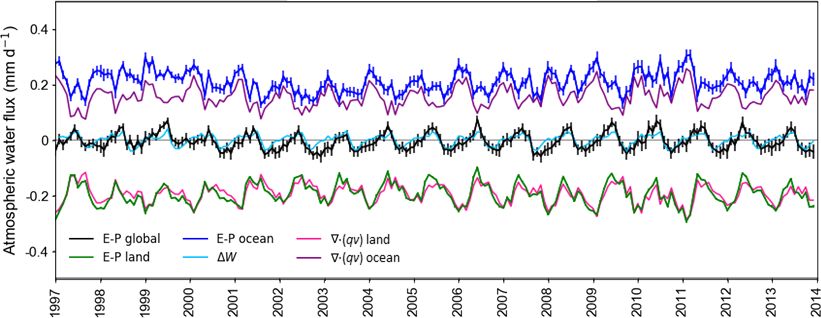
E − P , as shown in Fig. A2. 1W (light blue line) display a high degree of coherence, as
expected from Eq. (2). This is an indication that the (atmo-
4.4 Examination of the water budget in ERA5 spheric) water cycle is well represented in ERA5.
Globally, VIMD is zero, as no water vapor is transported
One way of investigating the consistency of different water out of (or into) the Earth system. However, we find ERA5
cycle components is determining if the global water budget global total VIMD to be −0.04 mm d−1 : a small value within
(Eq. 1) is closed. However, satellite E −P data sets are avail- the standard deviation of the ensemble of single grid boxes,
able over ocean only, so we revert to a comparison with gap- but significant and on the order of the amplitude of the
free reanalysis data. There is no internal constraint for bud- seasonal cycle of net E − P on a global scale. The de-
get closure in ERA reanalyses (Berrisford et al., 2011; Hers- viation from zero is due to the fact that VIMD is calcu-
bach et al., 2020), and as the budget was not closed in ERA- lated in grid point space (and not in the model’s spectral
Interim, it is worthwhile to investigate ERA5’s behavior in space), where the mathematical constraint of net zero di-
this regard. Monthly mean total ERA5 E − P over the globe, vergence is not enforced (Paul Berrisford, personal com-
the ocean, and land is shown in Fig. 7 in black, blue, and munication, October 2020). Interestingly, VIMD over land
green, respectively. The mean values over the globe and land (pink) agrees well with over-land E−P , whereas VIMD over
were scaled by their surface area relative to the ocean surface ocean (purple line) is smaller than over-ocean E − P also by
area (i.e., they were multiplied by 510/350 and 160/350, re- −0.04 mm d−1 . Based on the results of the regression anal-
spectively) to obtain consistency with the over-ocean means ysis shown in the upper panels of Fig. A2 we speculate that
shown in Fig. 3. The error bars on ERA5 data depict the stan- discrepancies between E − P and ∇ · (vq) over the ocean’s
dard deviation of the 10-member ensemble. Nearly all of the
uncertainty in global mean E − P is due to the uncertainty
https://doi.org/10.5194/hess-25-121-2021 Hydrol. Earth Syst. Sci., 25, 121–146, 2021You can also read