The retrieval of snow properties from SLSTR Sentinel-3 - Part 2: Results and validation
←
→
Page content transcription
If your browser does not render page correctly, please read the page content below
The Cryosphere, 15, 2781–2802, 2021
https://doi.org/10.5194/tc-15-2781-2021
© Author(s) 2021. This work is distributed under
the Creative Commons Attribution 4.0 License.

The retrieval of snow properties from SLSTR Sentinel-3
– Part 2: Results and validation
Linlu Mei1 , Vladimir Rozanov1 , Evelyn Jäkel2 , Xiao Cheng3 , Marco Vountas1 , and John P. Burrows1
1 Instituteof Environmental Physics, University of Bremen, Bremen, Germany
2 Leipzig Institute for Meteorology, University of Leipzig, Leipzig, Germany
3 School of Geospatial Engineering and Science, Sun Yat-Sen University, Zhuhai, 519082, PR China

Correspondence: Linlu Mei (mei@iup.physik.uni-bremen.de)

Received: 16 September 2020 – Discussion started: 7 October 2020
Revised: 15 May 2021 – Accepted: 18 May 2021 – Published: 18 June 2021

Abstract. To evaluate the performance of the eXtensible         (RMSEs) of SGS and SSA are around 12 µm and 6 m2 /kg.
Bremen Aerosol/cloud and surfacE parameters Retrieval           (2) For SPS, aggregate SPS retrieved by XBAER algorithm
(XBAER) algorithm, presented in the Part 1 companion pa-        is likely to be matched with rounded grains while single SPS
per to this paper, we apply the XBAER algorithm to the Sea      in XBAER is possibly linked to faceted crystals.
and Land Surface Temperature Radiometer (SLSTR) instru-            The comparison with aircraft measurements, during the
ment on board Sentinel-3. Snow properties – snow grain size     Polar Airborne Measurements and Arctic Regional Climate
(SGS), snow particle shape (SPS) and specific surface area      Model Simulation Project (PAMARCMiP) campaign held in
(SSA) – are derived under cloud-free conditions. XBAER-         March 2018, also shows good agreement (with R = 0.82 and
derived snow properties are compared to other existing satel-   R = 0.81 for SGS and SSA, respectively). XBAER-derived
lite products and validated by ground-based and aircraft        SGS and SSA reveal the variability in the aircraft track of the
measurements. The atmospheric correction is performed on        PAMARCMiP campaign. The comparison between XBAER-
SLSTR for cloud-free scenarios using Modern-Era Retro-          derived SGS results and the Moderate Resolution Imaging
spective Analysis for Research and Applications (MERRA)         Spectroradiometer (MODIS) Snow-Covered Area and Grain
aerosol optical thickness (AOT) and the aerosol typing strat-   size (MODSCAG) product over Greenland shows similar
egy according to the standard XBAER algorithm. The opti-        spatial distributions. The geographic distribution of XBAER-
mal SGS and SPS are estimated iteratively utilizing a look-     derived SPS over Greenland and the whole Arctic can be rea-
up-table (LUT) approach, minimizing the difference between      sonably explained by campaign-based and laboratory inves-
SLSTR-observed and SCIATRAN-simulated surface direc-            tigations, indicating a reasonable retrieval accuracy of the re-
tional reflectances at 0.55 and 1.6 µm. The SSA is derived      trieved SPS. The geographic variabilities in XBAER-derived
for a retrieved SGS and SPS pair. XBAER-derived SGS,            SGS and SSA both over Greenland and Arctic-wide agree
SPS and SSA have been validated using in situ measure-          with the snow metamorphism process.
ments from the recent campaign SnowEx17 during February
2017. The comparison shows a relative difference between
the XBAER-derived SGS and SnowEx17-measured SGS of
less than 4 %. The difference between the XBAER-derived         1   Introduction
SSA and SnowEx17-measured SSA is 2.7 m2 /kg. XBAER-
derived SPS can be reasonably explained by the SnowEx17-        Change in snow properties is both a consequence and a driver
observed snow particle shapes. Intensive validation shows       of climate change (Barnett et al., 2005). Snow cover and
that (1) for SGS and SSA, XBAER-derived results show high       snow season, especially in the Northern Hemisphere, are re-
correlation with field-based measurements, with correlation     ported by different models to decrease due to climate change
coefficients higher than 0.85. The root mean square errors      (Liston and Hiemstra, 2011). The reduction in snow cover
                                                                leads to a change in the surface energy budget (Cohen and

Published by Copernicus Publications on behalf of the European Geosciences Union.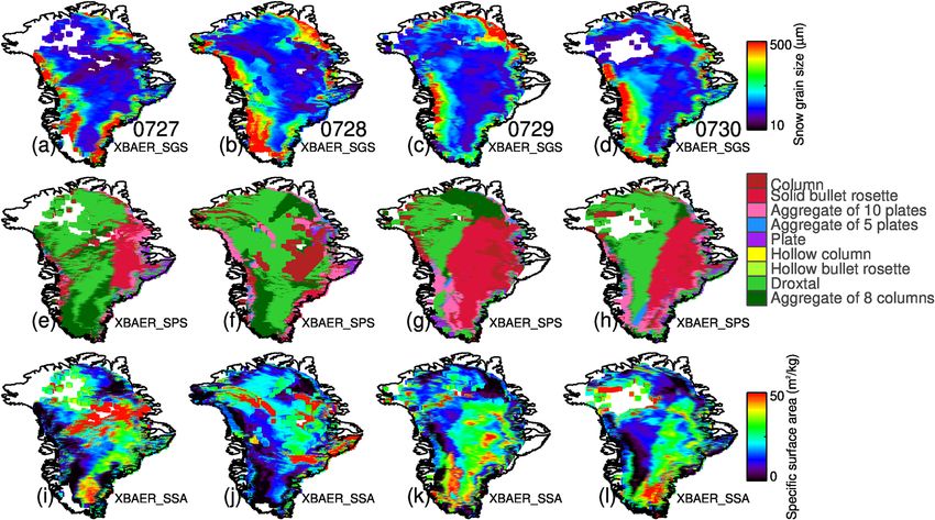
2782                                                   L. Mei et al.: The retrieval of snow properties from SLSTR Sentinel-3

Rind, 1991; Henderson et al., 2018), a reduction in Asian           al., 2009). The MODSCAG algorithm can provide the snow
summer rainfall (Liu and Yanai, 2002; Zhang et al., 2019),          cover fraction and snow albedo besides SGS on a pixel base.
a loss of Arctic plant species (Phoenix, 2018), and other im-       Topographic effects in MODSCAG are not considered, and
pacts on societies and ecosystems (Bokhorst et al., 2016).          the MODSCAG product tends to overestimate SGS (Mary
Snow may influence the climate through both direct and in-          et al., 2013). Other retrieval algorithms have also been de-
direct feedbacks (Lemke et al., 2007). The direct feedback          signed for and tested on the MODIS instrument (Stamnes et
is the snow–albedo feedback, and the indirect feedbacks in-         al., 2007; Aoki et al., 2007; Hori et al., 2007). Jin et al. (2008)
volve atmospheric circulation. The snow–albedo feedback             retrieved SGS over the Antarctic continent using MODIS
describes the mechanism by which melting snow (the ab-              data based on an atmosphere–snow coupling radiative trans-
sence of snow cover), caused by global warming, reflects less       fer model. Lyapustin et al. (2009) proposed a fast retrieval
solar radiation and further enhances the warming (Thackeray         algorithm for SGS at a 1 km spatial resolution using MODIS
and Fletcher, 2016). The snow indirect feedbacks describe           observations. The algorithm is based on an analytical asymp-
the impact of snow property change on monsoonal and an-             totic radiative transfer model. Negi and Kokhanovsky (2011)
nual atmospheric circulation (Lemke et al., 2007; Gastineau         proposed the use of the asymptotic radiative transfer (ART)
et al., 2017). However, the snow cover may be declining even        theory to retrieve SGS. The retrieved snow albedo and grain
faster than thought due to large uncertainties in how mod-          size from Negi and Kokhanovsky (2011) were validated and
els describe the snow feedback mechanisms (Flanner et al.,          showed good accuracy for clean and dry snow. However, po-
2011). The uncertainties in describing the snow feedback            tential problems have been reported for dirty snow (e.g., soot
mechanisms are largely introduced by the uncertainties in           and/or dust contamination). The Snow Grain Size and Pollu-
knowledge of snow properties (Hansen et al., 1984; Groot            tion (SGSP) algorithm retrieves SGS and pollution amount
Zwaaftink et al., 2011; Sarangi et al., 2019). Snow properties      based on a snow model (Zege et al., 1998), without a priori
depend on snow age, moisture, and surrounding temperatures          assumptions about SPS (Zege et al., 2011). The SGSP al-
(LaChapelle, 1969; Sokratov and Kazakov, 2012).                     gorithm has been validated using in situ measurements over
   Model simulations and field-based measurements provide           central Antarctica, and an underestimation of SGSP-derived
valuable information of snow properties (e.g., snow grain           SGS was reported under a large solar zenith angle (Zege et
size (SGS), snow particle shape (SPS), specific surface area        al., 2011; Carlsen et al., 2017). The algorithm is currently
(SSA)) for the understanding of changing snow and its cor-          implemented for the MODIS instrument and provides opera-
responding impact on climate change. Satellite observations         tional daily snow products (Wiebe et al., 2011). New instru-
offer another effective way to derive those snow properties         ments such as Hyperion on board Earth Observing-1 (EO-1)
on a large scale with a high quality (e.g., Painter et al., 2003,   and OLCI have also been used to derive SGS (Zhao et al.,
2009; Stamnes et al., 2007; Lyapustin et al., 2009; Wiebe           2013; Kokhanovsky et al., 2019). The algorithm proposed by
et al., 2013). The similarities and differences in the required     Kokhanovsky et al. (2019) is conceptually based on an ana-
snow parameters and their accuracy between the snow re-             lytical ART model, which estimates snow reflectance by the
mote sensing community and other communities (e.g., field           given SGS and ice absorption (Kokhaovksy et al., 2018). The
measurement community) are discussed in detail in the Part 1        snow grains in the ART model are described as a fractal.
companion paper (Mei et al., 2021a). In this paper, SGS (ef-           Snow particle shape is a fundamental parameter needed to
fective radius) is defined as 3V /(4Ap ), where V and Ap are        describe snow properties (Räisänen et al., 2017). The SPS
the volume and average projected area, respectively.                keeps relatively stable before falling on the ground under
   Different retrieval algorithms to derive SGS have been           cold and dry conditions, while it has large variabilities un-
developed for different instruments. The Airborne Visi-             der warm and wet conditions (Dang et al., 2016). The In-
ble/Infrared Imaging Spectrometer (AVIRIS) and Thematic             ternational Classification for Seasonal Snow on the Ground
Mapper (TM) on board Landsat are pioneer instruments used           (ICSSG) has grouped the SPS into nine main morphologi-
for the retrieval of SGS (Hyvarinen and Lammasniemi, 1987;          cal shapes: precipitation particles (PP), machine-made snow
Li et al., 2001). Painter et al. (2003, 2009) retrieved SGS         (MM), decomposing and fragmented (DF) precipitation par-
using AVIRIS and Moderate Resolution Imaging Spectro-               ticles, rounded grains (RG), faceted crystals (FC), depth hoar
radiometer (MODIS) data, exploring the information from             (DH), surface hoar (SH), melt forms (MF), and ice forma-
both visible and near-infrared spectral channels. There are         tions (IF) (Fierz et al., 2009). Another classification system,
several available satellite SGS products for MODIS (Klein           named “global classification” was proposed in Nakaya and
and Stroeve, 2002; Painter et al., 2009; Rittger et al., 2013)      Sekido (1938) and has been updated recently by Kikuchi
and its successor, the Visible Infrared Imaging Radiometer          et al. (2013). The global classification is obtained based on
Suite (VIIRS) (Key et al., 2013). For instance, the MODIS           the SPS. The information in Kikuchi et al. (2013) is quali-
Snow-Covered Area and Grain size (MODSCAG) product                  tatively used to understand the satellite-derived SPS in this
is created utilizing a spectral mixture analysis method based       paper. Due to the complexity of the ice crystal shape, sim-
on the prescribed endmember. The endmember is a spec-               plified ice crystal shapes, such as fractal (Macke et al., 1996;
trum library for snow, vegetation, rock, and soil (Painter et       Kokhanovsky et al., 2019) and droxtal (Pirazzini et al., 2015),

The Cryosphere, 15, 2781–2802, 2021                                                     https://doi.org/10.5194/tc-15-2781-2021
L. Mei et al.: The retrieval of snow properties from SLSTR Sentinel-3                                                         2783

have been used in some satellite retrievals and model sim-          rosette, hollow column, plate, aggregate of 5 plates, aggre-
ulations. However, previous investigations show that non-           gate of 10 plates, solid bullet rosette, column) (Yang et al.,
fractal snow types occur more frequently in reality (Gor-           2013) are used to describe the snow optical properties and to
don and Taylor, 2009; Comola et al., 2017). Information on          simulate the snow surface reflectance at 0.55 and 1.6 µm.
SPS, even limited or inaccurate, is extremely helpful and ur-          As mentioned in the Part 1 companion paper, the nine
gently needed for a better understanding of different snow          SPSs of Yang et al. (2013) used in the XBAER algorithm
types (Picard et al., 2009). The widely used spherical-shape        are proven to be a new option to describe the ice crystal lo-
assumption in field-based measurements (e.g., Flanner and           cal optical properties for the snow community (e.g., Saito et
Zender, 2006) is not optimal for satellite-oriented retrievals      al., 2019; Pohl et al., 2020; Mei et al., 2021b), and we would
because the spherical-shape assumption cannot produce the           also like to emphasize several more points to avoid misun-
angular distribution of snow reflectance with the required ac-      derstandings between different scientific communities.
curacy (Leroux and Fily, 1998; Jin et al., 2008; Dumont et             Difference between field-measured and satellite-derived
al., 2010; Mei et al., 2021b), which will introduce an unac-        SPS. A field-measured SPS is an optical shape for a single ice
ceptable magnitude of uncertainty in the satellite-retrieved        crystal, while satellite-derived SPS is an averaged radiative
snow properties. Some attempts to derive ice crystal shape          shape over a certain geographic area. The geographic area is
in ice clouds can be found in previous publications (Mc-            determined by the instrument spatial resolution (1 km is used
Farlane et al., 2005; Cole et al., 2014). However, there is         in this study). Thus it is unreasonable to directly compare
no publication with respect to the retrieval of the ice crystal     a kilometer average radiative shape to a single-ice-crystal
shape in the snow layer using passive multi-spectrum satellite      shape. However, for a region with a similar snow metamor-
observations. Although habit mixture models are preferable          phism process (Colbeck, 1980, 1983), the field-measured
for the description of snow grain shapes (Saito et al., 2019;       SPS may provide some representative information with re-
Tanikawa et al., 2020; Pohl et al., 2020), the information con-     spect to if the ice crystal shape is convex (e.g., spherical
tent from satellite observation is limited compared to field-       shape) or non-convex (aggregate shape), which is also crit-
based measurements. Thus, an optimal single shape, which            ical for further applications. This fundamental difference be-
provides the best agreement between simulation and satellite        tween field-measured and satellite-derived SPS means that
observation (e.g., top-of-atmosphere (TOA) reflectance), is         only a qualitative evaluation of the satellite-retrieved SPS is
also needed.                                                        possible. Please note that this spatial-resolution issue is more
   A few attempts have been proposed to retrieve SSA from           than just a typical “general scale issue” because it fully de-
spaceborne observations. The retrieval of SSA is actually           pends on the parameters retrieved, especially on their inho-
performed based on the pre-retrieved SGS with an assump-            mogeneity.
tion of a known SPS. Mary et al. (2013) retrieved SSA over             Requests to describe snow properties in the radiative
mountain regions using MODIS data, assuming a spherical             transfer theory. There is another way to describe snow prop-
ice crystal shape. The algorithm performs a topographic cor-        erties in the radiative transfer theory. This manner needs no
rection for the surface reflectance to achieve a better retrieval   knowledge with respect to SPS but uses an assumption of a
accuracy. The overall difference, compared to field measure-        stochastic medium. However, in this manner, there are also
ments, is 9.4 m2 /kg. Xiong and Shi (2018) retrieved SSA us-        parameters (e.g., mean photon path length) which cannot be
ing a snow reflectance model. The model simulates the light         validated. It is worth noticing that all manners, for the re-
scattering process using a Monte Carlo method and shows             trieval of snow properties from satellites, need to make some
an improvement in the bidirectional reflectance, thus a bet-        assumptions. These assumptions are fundamentally needed
ter retrieval accuracy of SSA, compared to the spherical as-        for a specific retrieval algorithm (Langlois et al., 2020).
sumption. The overall difference, compared to field measure-           Different radiative transfer models used for snow com-
ments, is about 6 m2 /kg.                                           munity. For the widely used asymptotic radiative transfer
   This paper, as in the Part 1 companion paper, applies the        (ART) model, even though the users do not highlight the is-
eXtensible Bremen Aerosol/cloud and surfacE parameters              sues linked to SPS, these issues exist. (1) The original ART
Retrieval (XBAER) algorithm to the Sea and Land Surface             model (Zege et al., 2004; Kokhanovsky and Zege, 2004) is
Temperature Radiometer (SLSTR) on board Sentinel-3 to de-           derived based on the assumption of a second-generation frac-
rive SGS, SPS and SSA. The general concept is to use the            tal for the ice crystal shape. (2) In the updated ART model
channels, which are sensitive to SGS and SPS, simultane-            (Kokhnaovsky et al., 2018), g and B parameters are intro-
ously. The channels used in XBAER algorithms are 0.55 and           duced. The g parameter depends on both SGS and SPS. The
1.6 µm. An optimal SGS and SPS pair is achieved by min-             B parameter depends strongly on SPS (Libois et al., 2014).
imizing the difference in atmosphere-corrected directional          Even though one can state that the g and B parameters can
surface reflectances between satellite observations and SCI-        be fitted to real observations, several issues linked to the as-
ATRAN simulations. SSA is then calculated based on the              sumption of SPS occur: (1) the accuracy of using a single g
retrieved SGS and SPS. Nine predefined ice crystal parti-           parameter to describe the complicated particle phase func-
cle shapes (aggregate of 8 columns, droxtal, hollow bullet          tion needs to be checked and (2) the ART model is designed

https://doi.org/10.5194/tc-15-2781-2021                                                  The Cryosphere, 15, 2781–2802, 2021
2784                                                  L. Mei et al.: The retrieval of snow properties from SLSTR Sentinel-3

for a medium with weak absorption properties; thus it can-
not be used for certain SGSs and SPSs, especially for long
wavelengths (e.g., 1.6 µm). In short, we cannot really avoid
making certain (explicit or hidden) assumptions about SPS
if it is not iteratively retrieved in the algorithm, like in the
XBAER algorithm.
   Highlighting with respect to the XBAER-retrieved SPS. We
believe our work, as a first step/attempt, provides a new and
useful approach and some new and useful information for
the SPS. However, we should not over-interpret the shape we
retrieved.
   This paper is structured as follows: instrument characteris-
tics of SLSTR and the field-based measurements and aircraft        Figure 1. Geographic distribution of the validation sites. The colors
measurements used for validation are described in Sect. 2.         represent the type of each site, and the site name used in this paper
                                                                   is indicated near each site.
Section 3 describes the method including cloud screening,
atmospheric correction and the flowchart of the XBAER al-
gorithm. Some selected data products and comparisons with
MODIS products and field-based measurements are shown              ments because of cloud coverage. This paper focuses on the
in Sect. 4. The comparison with the recent campaign mea-           Sentinel-3a satellite for the periods of February 2016 (launch
surement is presented in Sect. 5. A discussion to illustrate a     month of Sentinel-3a) and December 2020. The field-based
time series of the retrieval results is shown in Sect. 6. The      measurements from both permanent sites and campaign sites
conclusions are given in Sect. 7.                                  for the focal time period are collected. Figure 1 shows the ge-
                                                                   ographic distribution of the validation sites. The site names
                                                                   used in this paper are listed near each site. Since XBAER re-
2     Data                                                         trieves SGS, SPS and SSA simultaneously, the SnowEx cam-
                                                                   paign, which provides the three parameters as well, will be
2.1    SLSTR instrument
                                                                   introduced in detail first.
After the loss of Environmental Satellite (Envisat) on                The National Aeronautics and Space Administration
12 April 2012, the European Space Agency (ESA)                     (NASA) established a terrestrial hydrology program
launched Sentinel-3A and Sentinel-3B in February 2016              (SnowEx mission) in order to better quantify the amount of
and April 2018, respectively. As the successor of Advanced         water stored in snow-covered regions (Kim et al., 2017). The
Along-Track Scanning Radiometer (AATSR) on board En-               measurements for the first year (2016–2017) were carried
visat, Sentinel satellites take the SLSTR instrument. The          out during February 2017 (between 8 and 25 February 2017)
SLSTR instrument has similar characteristics to AATSR (see         at Grand Mesa and the Senator Beck Basin in Colorado
Table 1 for details). The instrument has nine spectral bands       (hereafter referred to as SnowEx17) (see Fig. 2a) (Elder
in the visible and infrared spectral range. It also has dual-      et al., 2018). Grand Mesa is a forest region covered by
view observation capability with swath widths of 1420 and          relatively homogeneous snow cover with an area size similar
750 km for nadir and oblique directions, respectively. The         to airborne instrument swath widths (Brucker et al., 2017)
SLSTR and AATSR dual-view observations of the Earth’s              (see Fig. 2c). The Senator Beck Basin site has complex
surface make surface bidirectional reflectance distribution        topography and is covered by snow. The campaign used
function (BRDF) effect estimation possible, which is widely        more than 30 remote sensing instruments, and most of the
used to retrieve both surface and atmospheric geophysi-            instruments are from the NASA except some instruments
cal parameters (Popp et al., 2016). Besides the heritage of        such as ESA’s radar (Kim et al., 2017). The snow pit
AATSR, some new features (wider swath, new spectral bands          measurements provide information on snow grain size and
and higher spectral resolution for certain bands) have been        type/shape, stratigraphy profiles, and temperatures with
included in SLSTR instrument (https://sentinel.esa.int/web/        certain information about surface conditions (e.g., snow
sentinel/technical-guides/sentinel-3-slstr/instrument, last ac-    roughness) (Rutter et al., 2018). The SnowEx17 campaign
cess: 13 June 2021).                                               provides seven different shapes (new snow, rounds, facets,
                                                                   mixed forms, melt–freeze, crust and ice lens). Table 2
2.2    Ground-based measurements                                   lists both the SnowEx17-measured snow grain shapes and
                                                                   SPSs defined in Yang et al. (2013). The SPSs defined by
The validation of satellite-derived snow properties is chal-       ICSSG are also listed in the table, and the possible linkage
lenging due to (i) limited available field-based measure-          between Yang et al. (2013) SPS and ICSSG SPS (named SPS
ments and (ii) the difficulties of spatial–temporal colloca-       similarity) will be discussed later. The measurements have
tion between satellite observations and field-based measure-       been publicly released at http://nsidc.org/data/snowex (last

The Cryosphere, 15, 2781–2802, 2021                                                     https://doi.org/10.5194/tc-15-2781-2021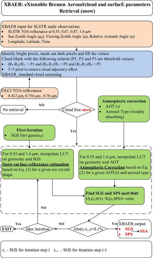
L. Mei et al.: The retrieval of snow properties from SLSTR Sentinel-3                                                        2785

Table 1. Instrument characteristics of AATSR and SLSTR.

                                          SLSTR                                     AATSR
                         Band     Central wavelength    Resolution   Band    Central wavelength   Resolution
                         no.                    (µm)          (m)     no.                  (µm)         (m)
                         1                     0.555           500      4                0.555         1000
                         2                     0.659           500      5                0.659         1000
                         3                     0.865           500      6                0.865         1000
                         4                     1.375           500
                         5                     1.610           500      7                1.610         1000
                         6                      2.25           500
                         7                      3.74          1000      1                 3.74         1000
                         8                     10.85          1000      2                10.85         1000
                         9                        12          1000      3                   12         1000
                         10                     3.74          1000
                         11                    10.85          1000

                                                                        The SPS and SSA measurements around Inuvik, North-
                                                                     west Territories of Canada (68.73◦ N, 133.49◦ W), cover the
                                                                     period of November 2018–March 2019. There were three de-
                                                                     ployments, the freeze-up period (November 2018), the storm
                                                                     input period (January 2019) and the metamorphosis period
                                                                     (March 2019) (King et al., 2019).
                                                                        The SSA measurements above the French Alps (45.04◦ N,
                                                                     6.41◦ W) were collected in the snow seasons during 2016–
                                                                     2018 (Tuzet et al., 2020). The measurements for the 2016–
                                                                     2017 period provide SSA profile information with a vertical
                                                                     resolution of 3 cm using the DUFISSS instrument (Gallet et
                                                                     al., 2009). For the period of 2017–2018, the measurements
                                                                     were obtained with a vertical resolution of 6 cm using the
                                                                     Alpine Snowpack Specific Surface Area Profiler (Libois et
Figure 2. Photos taken during the SnowEx campaign. (a) An            al., 2014). The uncertainty is estimated to be 10 %.
overview of the campaign environment around the Senator Beck            The SGS measurements were obtained over Nagaoka,
Basin site. (b) Location of the SnowEx campaign (red rectangles).
                                                                     Japan (37.41◦ N, 138.88◦ W) (Yamaguchi et al., 2019;
(c) An overview of the campaign environment around the Grand
                                                                     Avanzi et al., 2019). The observations during January 2017–
Mesa site. (Credit: Roy A. Langlois and Lisa Brucker at the Na-
tional Snow and Ice Data Center, University of Colorado, Boulder.)   March 2018 are used in this paper.
                                                                        The SGS measurements were obtained over Xinjiang
                                                                     province during a different period (Chen et al., 2020); the
                                                                     dataset around the site (44.146◦ N, 85.848◦ E) for the period
access: 13 June 2021). The data were collected in SnowEx20           November 2018–November 2019 is used in this paper.
for the period of 27 January and 12 February 2020.                      The SSA measurements at Dome C (75◦ S, 123◦ E) in
   The measurements over Greenland are obtained by the               Antarctica cover the period of 2016–2018, and the accuracy
EastGRIP team over 75.63◦ N, 36.004◦ W. Detailed informa-            of the measurements is better than 15 % (Picard et al., 2016).
tion about the site can be found at https://eastgrip.org (last       The data were collected using a self-designed and assembled
access: 13 June 2021). The data have been used to validate           instrument, named Autosolexs, which can be used to mea-
the SGS and SSA derived from OLCI (Kokhanvosky et al.,               sure the snow properties for several years under the harsh
2018). The same dataset, covering the period of May 2017             environment.
and August 2018 is used in this paper. SGS or SSA is calcu-
lated using the relationship between SSA and SGS if SSA or           2.3    Aircraft observations
SGS is not measured.
   The SSA measurements at Nunavut, northern Canada                  During the Polar Airborne Measurements and Arctic Re-
(69.20◦ N, 104.80◦ W), were obtained using the instrument            gional Climate Model Simulation Project (PAMARCMiP)
described by Montpetit et al. (2012). The observation period         campaign held in March and April 2018, ground-based and
covers April 2018.                                                   airborne observations of surface, cloud and aerosol proper-

https://doi.org/10.5194/tc-15-2781-2021                                                    The Cryosphere, 15, 2781–2802, 2021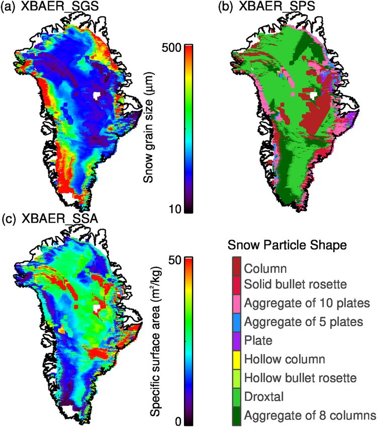
2786                                                   L. Mei et al.: The retrieval of snow properties from SLSTR Sentinel-3

Table 2. Snow grain type (shape) provided by Yang et al. (2013), in situ measurements in the SnowEx campaign and by ICSSG. Please note
here the grain type by Yang et al. (2013) measured in SnowEx and provided by ICSSG given in the same line have no 1 : 1 linkage.

ties were performed near the Villum Research Station (North          applied according to the procedure described by Wendisch et
Greenland). One of the most important objectives of the              al. (2004). The retrieval of the snow grain sizes is based on
PAMARCMiP 2018 campaign was to quantify the physical                 the method described in Carlsen et al. (2017) which uses a
and optical properties of snow, sea ice and the atmosphere           modified approach presented by Zege et al. (2011).
(Egerer et al., 2019; Nakoudi et al., 2020). Airborne spec-
tral irradiance measurements by the Spectral Modular Air-
borne Radiation Measurement System (SMART) on board                  3     Methodology
the Polar 5 research aircraft operated by the Alfred-Wegener-
Institut were used to derive snow grain sizes along the flight       3.1    Cloud screening
track. The SMART provides solar up- and downward spec-
tral irradiances in the range between 0.4–2.0 µm. The optical        The algorithm synergistically uses SLSTR and OLCI data to
inlets are actively horizontally stabilized with respect to air-     identify clouds over the snow surface. The criteria for cloud
craft movement (Wendisch et al., 2001) within 5◦ pitch and           screening over snow using SLSTR and OLCI measurements
roll angles. In particular, for high solar zenith angles (SZAs)      can be found in Istomina et al. (2010) and Mei et al. (2017),
as presented during PAMARCMiP (about an 80◦ SZA), mis-               respectively. Short summaries of Istomina et al. (2010) and
alignment of the optical inlets implies significant measure-         Mei et al. (2017) are presented below, and more details can
ment uncertainties (Wendisch et al., 2001). Further uncer-           be found in the original publications. The algorithm proposed
tainties are related to the spectral and radiometric calibra-        by Istomina et al. (2010) for the SLSTR instrument utilizes
tion, as well as to the correction of the cosine response which      spectral behavior differences at SLSTR visible and thermal
sums to a total wavelength-dependent uncertainty (1 sigma)           infrared channels, and this algorithm was updated later by
for the irradiances ranging between 3 % and 14 % (Jäkel et           Jafariserajehlou et al. (2019). Relative thresholds are deter-
al., 2015). The derivation of the surface albedo from aircraft       mined based on radiative transfer simulations under various
observations requires atmospheric corrections due to the at-         atmospheric and surface conditions. The method proposed
mospheric attenuation and scattering by gases and aerosols.          by Mei et al. (2017b) for the OLCI instrument uses differ-
Therefore an iterative method to correct for these effects was       ent cloud characteristics: cloud brightness, cloud height and

The Cryosphere, 15, 2781–2802, 2021                                                      https://doi.org/10.5194/tc-15-2781-2021
L. Mei et al.: The retrieval of snow properties from SLSTR Sentinel-3                                                                         2787

cloud homogeneity. The TOA reflectance at 0.412 µm, the ra-                          as weakly absorbing according to a previous investigation
tio of TOA reflectance at 0.76 and 0.753 µm, and the standard                        (Mei et al., 2020b).
deviation of TOA reflectance at 0.412 µm are used to charac-
terize cloud brightness, cloud height and cloud homogene-                            3.3    XBAER algorithm
ity, respectively. A pixel is identified as a cloud-free snow
pixel when both SLSTR and OLCI identify it as a cloud-                               The theoretical background of the retrieval algorithm is
free snow pixel. Identified clouds can be surrounded by a so-                        given in Sect. 4 of the companion paper. The XBAER algo-
called “twilight zone” (Koren et al., 2007), which can extend                        rithm consists of three stages to derive SGS, SPS and SSA:
more than 10 km from a cloud pixel to a cloud-free area. The                         (1) derivation of SGSs for each predefined SPS, (2) selec-
surrounding 5 × 5 pixels of an identified cloud pixel will be                        tion of the optimal SGS and SPS pairs for each scenario, and
marked as a cloud to avoid the twilight zone effect. A more                          (3) calculation of SSA for each retrieved SGS and SPS. This
detailed description of this cloud screening method can be                           section describes some implementation details such as the se-
found in Mei et al. (2020a). Additionally, TOA reflectance at                        lection of the first guess for the retrieval parameters and the
0.55 µm is required to be higher than 0.5 to avoid dark ice                          flowchart of the algorithm.
and dirty snow.                                                                         A reasonable first-guess value for the iteration process
                                                                                     can significantly reduce the computation time, which is im-
3.2    Atmospheric correction                                                        portant for retrievals of atmospheric and surface proper-
                                                                                     ties over large geographic and temporal scales with differ-
Due to the low atmospheric aerosol loading over the Arc-                             ent instrument spatial resolutions. The first guess of SGS
tic snow-covered regions (e.g., Greenland), atmospheric cor-                         in the XBAER algorithm is obtained employing the semi-
rection using path radiance representation (Chandrasekhar,                           analytical snow reflectance model (Kokhanovsky and Zege,
1950; Kaufman et al., 1997) can provide accurate estima-                             2004; Kokhanovsky et al., 2018). Details of using this model
tion of surface reflection even under relatively large SZAs                          to derive SGS can be found in Lyapustin et al. (2009). Due to
(Lyapustin, 1999). The TOA reflectance at selected channels                          the different band settings in MODIS and SLSTR (SLSTR
(0.55 and 1.6 µm) is described by the path radiance represen-                        has no 2.1 µm channel like MODIS), one non-absorption
tation (Chandrasekhar, 1950; Kaufman et al., 1997) as                                channel (0.55 µm) and one absorption channel (1.6 µm) are
                                                                                     used in our SLSTR retrieval algorithm.
R(θ, θ0 , ϕ, τ, AT) = R 0 (θ, θ0 , ϕ, τ, AT)                                            Figure 3 shows the flowchart of how XBAER derives
       T (θ, θ0 , τ, AT)A                                                            SGS, SPS and SSA. The flowchart includes pre-processing of
   +                      ,                                                    (1)
        1 − s(τ, AT)A                                                                cloud screening using the synergy of OLCI and SLSTR and
                                                                                     the atmospheric correction using MERRA providing AOT
where R 0 (θ, θ0 , ϕ, τ, AT) is the TOA reflectance calculated                       and a weakly absorbing aerosol type. The SGS and SPS are
assuming a black surface (surface reflectance equals 0) un-                          obtained using the LUT-based minimization routine. SSA is
der a viewing zenith angle (VZA), solar zenith angle (SZA)                           then calculated using the retrieved SGS and SPS.
and relative azimuth angle (RAA) of θ, θ0 and ϕ. τ and AT
are aerosol optical thickness (AOT) and aerosol type (Mei
et al., 2017a). T (θ, θ0 , τ, AT) is the total (diffuse and direct)                  4     Results and comparison
transmittance from the sun to the surface and from surface
to the satellite; s(τ, AT) is spherical albedo; A is Lambertian                      Greenland is the largest ice-covered land mass in the North-
surface albedo. The spherical albedo is the fraction of the in-                      ern Hemisphere and the biggest cryospheric contributor to
cident solar radiation diffusely reflected over all directions                       the global sea-level rise (Ryan et al., 2019). XBAER-derived
(albedo of an entire planet). The Lambertian surface albedo                          SGS, SPS and SSA over Greenland enable a good under-
is defined as the ratio of reflected to incident flux. The at-                       standing of the retrieval accuracy with a large and repre-
mospheric correction is performed based on the following                             sentative geographic scale. Kokhanovsky et al. (2019) re-
equation:                                                                            ported that July is an optimal month to analyze satellite-
                                                                                     derived snow properties over Greenland because Greenland
A=                                                                                   has a strong snow particle metamorphism process (SPMP)
                R(θ, θ0 , ϕ, τ, AT) − R 0 (θ, θ0 , ϕ, τ, AT)
                                                                                     due to higher temperatures in July (Nakamura et al., 2001).
                                                                           .   (2)   The SPMP, affected strongly by temperature, is a dominant
(R(θ, θ0 , ϕ, τ, AT) − R 0 (θ, θ0 , ϕ, τ, AT))s(τ, AT) + T (θ, θ0 , τ, AT)
                                                                                     factor for the variabilities in SGS, SPS and SSA (LaChapelle,
The atmospheric correction is based on the look-up table                             1969; Sokratov and Kazakov, 2012; Saito et al., 2019). Snow
(LUT) pre-calculated using the radiative transfer code SCI-                          particle size increases dramatically and the ice crystal parti-
ATRAN (Rozanov et al., 2014). The radiative transfer cal-                            cles are compacted in the strong SPMP (Aoki et al., 1999;
culations were performed assuming AOT values provided by                             Nakamura et al., 2001; Ishimoto et al., 2018).
Modern-Era Retrospective Analysis for Research and Appli-
cations (MERRA) simulations, and aerosol type was defined

https://doi.org/10.5194/tc-15-2781-2021                                                                   The Cryosphere, 15, 2781–2802, 2021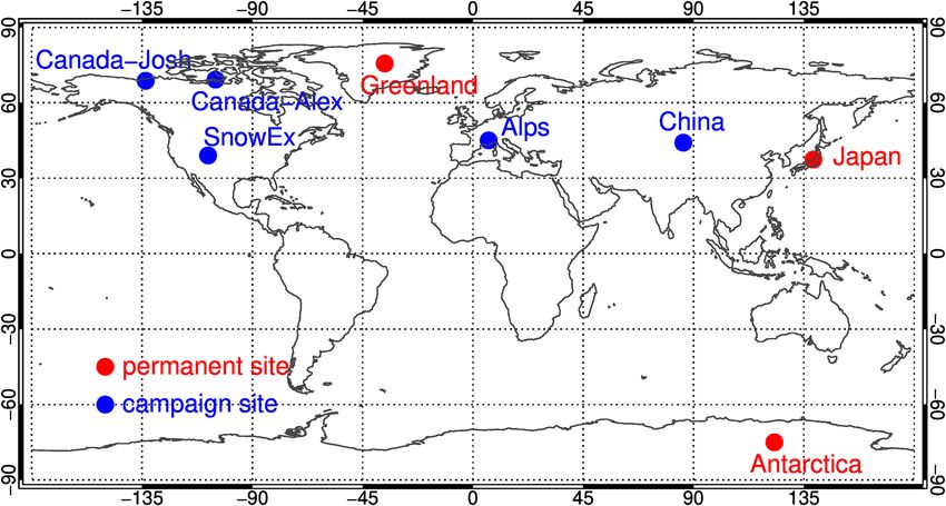
2788 L. Mei et al.: The retrieval of snow properties from SLSTR Sentinel-3
ular, central Greenland has a significantly higher elevation,
and the impacts of imperfect atmospheric correction on re-
trieved snow properties are ignorable. The lower temperature
under higher-elevation regions has a weaker SPMP, produc-
ing more irregular SPS. The opposite situation is the case in
the coastline regions over Greenland. Since Fig. 4 is com-
posited by three different SLSTR orbits, the geometrically
shaped features in eastern Greenland are caused by the effec-
tive Lambertian albedo assumption in the XBAER algorithm.
This assumption introduces additional bias under large view-
ing zenith angle conditions, which occurs at the edge of each
SLSTR orbit.
Figure 5 shows XBAER-retrieved SGS, SPS and SSA for
28 July 2017. Since there are no available products of SPS
and SSA from MODSCAG, it is a great challenge to make
a similar comparison to that in the case of SGS. Fortunately,
campaign-based and laboratory investigations provide valu-
able information on typical snow shapes at different times
and locations with a wide range of atmospheric conditions.
According to Kikuchi et al. (2013), the typical SPSs in the
polar regions include column crystal (e.g., solid column,
bullet-type crystal) with SGSs of about 50 µm for solid col-
umn and between 100 and 500 µm for bullet type, and the
germ of ice crystal group with SGSs of less than 50 µm.
Saito et al. (2019) pointed out that SPSs of fresh snow in
the polar regions are typically a mixture of irregular shapes
such as column and plate-like. Ishimoto et al. (2018) found
that aged snow can have an aggregate structure. The optical
properties of small ice crystal particles in aged snow may be
well-characterized by granular/roundish shapes, while SPSs
tend to be irregular or severely roughened shapes during the
SPMP (Ishimoto et al., 2018). Pirazzini et al. (2015) investi-
gated the impact of ice crystal sphericity on the estimation of
snow albedo and found droxtal is a reasonable assumption to
take ice particle non-sphericity into account. The above con-
Figure 3. Flowchart of the XBAER retrieval algorithm. clusions can be used as a qualitative reference to understand
the satellite-derived SPS. In the meantime, a large proportion
of ice sheet melts during the warm July, which unequivocally
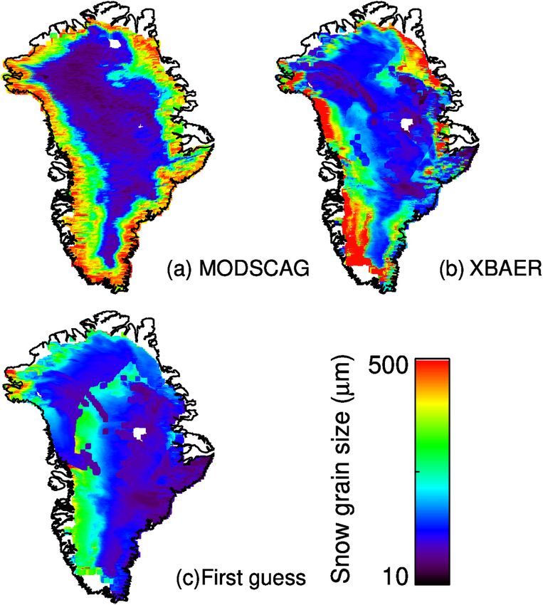
Figure 4 shows an example of the XBAER-derived SGS leads to rounded coarse grains very quickly. According to
on 28 July 2017 from SLSTR, XBAER first guess, and its Fig. 5, central Greenland is largely covered by small parti-
comparison with the same scenario from the MODSCAG cles with a roundish/droxtal shapes, while coastline regions
product (Painter et al., 2009). Here we chose MODIS on are covered by particles with aggregated shapes (aggregate
Aqua rather than MODIS on Terra to avoid the impact of of 8 columns, aggregate of 5 plates, aggregate of 10 plates)
instrument degradation of MODIS on Terra (Lyapustin et al., with large particle sizes, which is essentially attributed to
2014). The visualization of XBAER-derived SGS is shown the different SPMPs over different regions of Greenland.
to be between 10 and 500 µm. The XBAER first guess has Bullet-type crystal (solid bullet rosette) occurred with SGSs
in general a low value (Lyapustin et al., 2009) as com- of about 100 µm. The examples shown in Fig. 5 can be rea-
pared to XBAER and MODSCAG results. The XBAER- and sonably explained by previous publications (Kikuchi et al.,
MODSCAG-derived SGSs show good agreement on the ge- 2013; Pirazzini et al., 2015; Ishimoto et al., 2018; Saito et
ographic distribution. The slight difference in cloud-covered al., 2019).
regions (white parts) is explained by the different overpass The geographic distribution of SSA is somehow anti-
time between SLSTR and MODIS. Both algorithms demon- correlated with the geographic distribution of SGS, due
strate that SGSs in central Greenland are smaller than those to the definition of SSA. Most SSAs fall into the range
at coastline regions. This is attributed to the geographic dis- of 10–40 m2 /kg, which agrees with previous publication
tribution of surface temperature over Greenland. In partic- (Kokhanovsky et al., 2019). A change in SSA occurs espe-
The Cryosphere, 15, 2781–2802, 2021 https://doi.org/10.5194/tc-15-2781-2021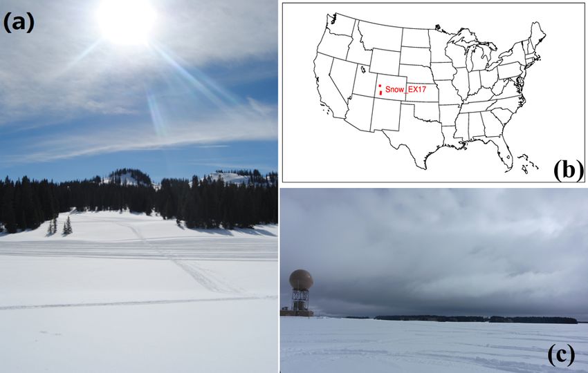
L. Mei et al.: The retrieval of snow properties from SLSTR Sentinel-3 2789
cially after snowfall (Carlsen et al., 2017; Xiong and Shi,
2018). Since SSA contains information on both SGS and SPS
and field measurements provide SSA, the validation of SSA
can be also used as “indirect quantitative validation” of SPS,
which will be quantitatively presented in the next section.
5 Validation
In this section, we will quantitatively validate XBAER-
derived snow properties with field-measured data and aircraft
measurements.
5.1 Validation using the observations of the SnowEx17
campaign
In order to have a quantitative evaluation of XBAER-derived
SGS, SPS and SSA, we have collocated the SLSTR ob-
servations with recent campaign measurements provided by
SnowEx17 and SnowEx20, as described in Sect. 2. Due
to overpass time and cloud cover, only limited match-ups
between XBAER retrievals and SnowEx17 and SnowEx20
measurements have been obtained. No match-up is obtained Figure 4. A comparison of the MODSCAG SGS (a), XBAER-
for SnowEx20. derived SGS (b) and first guess (c) over Greenland on 28 July 2017.
Table 3 summarizes match-up information. The first three
columns in Table 3 show the observation times and loca-
tions (longitude and latitude). The fourth and fifth columns
indicate the cloud conditions. Cloud conditions in Ta-
ble 3 are given in three categories: cloud-free snow, cloud-
contaminated snow and cloud-covered snow. These three cat-
egories are classified by the XBAER cloud identification re-
sults (see Sect. 3.1) and are illustrated by the RGB compo-
sition figures, covering the SnowEx campaign area, as pre-
sented in Fig. 6. An optically thin cloud over a melting snow
layer, a thick cloud over snow and snow scenarios are pre-
sented in Fig. 6a, b and c, respectively. The cloud optical
thickness (COT), estimated using the independent XBAER
cloud retrieval algorithm, as presented in Mei et al. (2018),
is ∼ 0.5 and ∼ 10 for 9 and 11 February, respectively.
Even though the synergistical use of SLSTR and OLCI
provides valuable information for separating cloud and snow,
the identification of an optically thin cloud above a snow
layer is a great challenge due to the similar wavelength de-
pendence of snow and cloud reflectance, especially between
snow and ice cloud (Mei et al., 2020b). The identification of
the cloud from an underlying snow layer in XBAER relies
mainly on the O2 channel of the OLCI instrument, which
provides the cloud height information (Mei et al., 2017b).
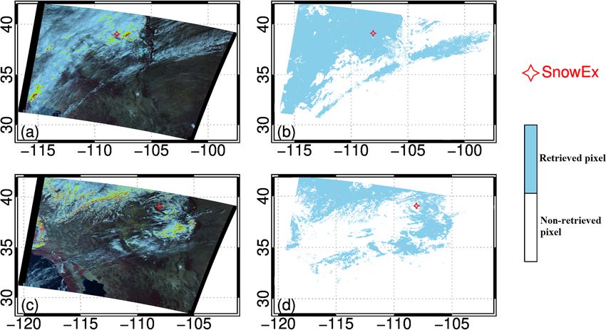
Figure 7 shows the performance of XBAER cloud identifica-
tion results for cloud contamination and cloud-covered snow
scenarios. The red star indicates the measurement location.
The zoomed-in images around the measurement site are pre-
Figure 5. XBAER-derived SGS, SPS and SSA over Greenland for
sented in Fig. 6. XBAER cloud screening shows, in general,
the same scenario as in Fig. 4.
good performance according to the RGB visual interpreta-
tion. However, part of the thin cirrus cloud on the 9 Febru-
https://doi.org/10.5194/tc-15-2781-2021 The Cryosphere, 15, 2781–2802, 2021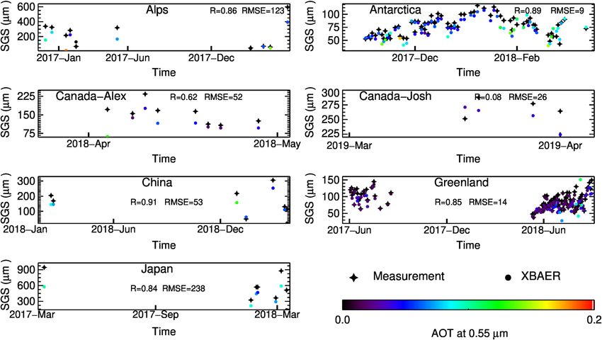
2790                                                       L. Mei et al.: The retrieval of snow properties from SLSTR Sentinel-3

Table 3. Information of match-ups between SnowEx and SLSTR during February 2017.

                                  Date         Long (◦ )     Lat (◦ )   COT     Comment
                                  9 Feb     −108.1092       39.0369     ∼ 0.5   cloud-contaminated snow
                                  11 Feb    −108.0462       39.0278     ∼ 10    cloud-covered snow
                                  22 Feb    −108.0634       39.0444         0   cloud-free snow
                                  22 Feb    −108.0625       39.0459         0   cloud-free snow
                                  22 Feb    −108.0617        39.047         0   cloud-free snow

Figure 6. Zoom of the RGB composition figures (created using
ESA official SLSTR software SNAP) for the three selected dates
presented in Table 3. The yellow point indicates the SnowEx instru-
ment position.
                                                                         Figure 7. The RGB composition (a, c) for 9 (a) and 22 (c) February
                                                                         when XBAER detected cloud-free snow and provided the retrieval.
                                                                         The XBAER cloud screening results (b, d) for the corresponding
ary is not correctly avoided. For 9 February, XBAER cloud                days are given in (b) and (d). “Retrieved pixel” refers to cloud-
identification gives a result of clean snow while it contains a          free snow. “Non-retrieved pixel” refers to the area where XBAER
thin cloud above a snow layer. For the 11 February, XBAER                retrieval is not performed; this includes (1) snow-free and cloud-
has successfully detected the cloud from an underlying snow              free, (2) cloud above snow, and (3) cloud above snow-free.
layer. For a comprehensive investigation of XBAER-derived
snow properties under all snow–cloud-coupled conditions,
the match-up on 11 February 2017 (shown in grey) has been                surements, especially for the 22 February. The average ab-
manually set to “cloud-free snow”. The reason for perform-               solute difference is less than 10 µm (4 % in relative differ-
ing the validation for different cloud conditions is that the            ence). The relatively large SGS (≥ 250 µm) caused mainly
satellite retrieval can only be performed under cloud-free               by the warm-up on the 21 February (see the comment in Ta-
conditions, while field measurements may be obtained un-                 ble 5, reported by campaign participators) led to a quicker
der cloud conditions, especially when fresh snow proper-                 snow metamorphism process, forming large ice crystal parti-
ties are measured. Thus, the field-based measurements un-                cles. MODSCAG only provides retrieval results for 9 and 11
der full-cloud or partly cloudy conditions are still valuable in         February. The results from XBAER and MODSCAG agree
the validation process (Jeoung et al., 2020). According to the           well. This possibly indicates similar performance between
sensitivity study, cloud contamination leads to an underesti-            XBAER and MODSCAG.
mation of SGS and the overestimation of SSA, depending on                   An underestimation is found for the first match-up on the
the cloud fraction.                                                      9 February. This is explained by the cirrus cloud contami-
   Table 4 summarizes the comparison between XBAER re-                   nation as presented in Fig. 11. According to an independent
trieval results, the MODSCAG product and SnowEx17 cam-                   XBAER cloud retrieval (Mei et al., 2018), the COT is ∼ 0.5;
paign measurements. The first three columns in Table 4                   cloud contamination with a COT of 0.5 introduces a ∼ 30 %
are the same as those of Table 3, showing the observa-                   underestimation according to Fig. 11 in the Part 1 companion
tion time and locations (longitude and latitude). The second             paper. So for SGS = 100 µm, provided by SnowEx, XBAER
three columns are the SnowEx17-measured SGS. Since the                   is expected to have a theoretically retrieved SGS of ∼ 70 µm,
SnowEx17 provides the SGS profile up to a 1 m depth, the                 while a value of 78.2 µm is obtained from the real satellite re-
minimum (SnowEx_min), average (SnowEx_avg) and max-                      trieval. In order to further confirm this negative bias feature
imum (SnowEx_max) values of SGS are listed in Table 3.                   caused by cloud contamination, the 11 February retrieval (a
The last two columns are MODSCAG- and XBAER-derived                      snowstorm at the measurement site is reported by campaign
SGS. For the four cloud-filter-passed match-ups, XBAER-                  participators), although filtered by the XBAER cloud screen-
derived SGS shows good agreement with SnowEx17 mea-                      ing routine, is forced to retrieve the fully cloud-covered sce-

The Cryosphere, 15, 2781–2802, 2021                                                          https://doi.org/10.5194/tc-15-2781-2021
L. Mei et al.: The retrieval of snow properties from SLSTR Sentinel-3 2791
nario as a cloud-free case. According to the theoretical in- Table 6 shows the comparison of SSA. For the three
vestigations presented in the Part 1 companion paper, for cloud-free samples, the difference in XBAER-derived SSA
COT ≥ 5, the XBAER algorithm retrieves the cloud effective and SnowEx17-measured SSA is 2.7 m2 /kg, which is sig-
radius rather than SGS. The retrieved ice crystal size depends nificantly smaller than what has been reported by previous
on the cloud effective radius of the cloud above the under- publications. For instance, the differences between satellite
lying snow layer. The independent XBAER cloud retrieval retrievals and field measurements are reported to be 9 and
provides an SGS value of ∼ 38, while 32.3 µm is obtained by ∼ 6 m2 /kg in Mary et al. (2013) and Xiong and Shi (2018).
the XBAER snow retrieval, for a reference value of 100 µm An interesting case is observed for the two samples on
as provided by SnowEx17 measurement. This is consistent 22 February. The SGSs show the same values for these two
with a typical ice cloud effective radius (King et al., 2013; match-ups (both are 254.4 µm from XBAER and 250 µm
Mei et al., 2018) under a snowstorm condition. from SnowEx); however, ground-based measurement shows
Table 5 shows the same match-up information as in Ta- almost 2 times the difference in SSA (29.8 vs. 14.6 m2 /kg)
ble 4 but for SPS. We would like to highlight again that the for these two samples, which is due to the different SPSs.
SPSs proposed by Yang et al. (2013) are used for the radia- SnowEx shows that the SPSs are new snow and facets for
tive transfer calculation. From a single-ice-crystal point of these two samples, respectively. XBAER-derived SSAs are
view, those shapes are very unlikely to occur exactly in re- 24.5 and 12.9 m2 /kg, which agrees well with SnowEx mea-
ality. This is similar to the issue in field measurements. In surement. Since both SnowEx and XBAER provide very sim-
field-based measurements, a spherical-shape assumption is ilar SGSs (250 µm vs. 254.4 µm), the agreement of SSA indi-
widely used (e.g., the calculation of SSA from SGS); how- cates that XBAER-derived aggregate of 8 columns is com-
ever, a pure spherical shape is also very unlikely to occur parable to “new snow”, while XBAER-derived droxtal is
in natural snow. To have a reasonable comparison between somehow “identical” to facets in SnowEx. Cloud contami-
satellite-derived SPS and field-measured SPS, the quantita- nation introduces an overestimation of SSA, especially for
tive information of “roundish” or “irregular” shapes from 11 February. According to the investigation from the com-
both satellite and field measurement communities may be an panion paper, for reference SSAs of 37.3 and 25.9 m2 /kg,
option. Under this comparison strategy, a “droxtal” shape de- SSA is expected to be ∼ 65 and > 100 m2 /kg for cloud con-
rived from satellite observation is somehow identical with a tamination with COT ∼ 0.5 and 10, respectively. The real
“spherical shape” in field measurement. satellite retrieval values are 56.5 and 136.8 m2 /kg.
The second and third columns in Table 5 show SnowEx17- The above validation for the retrieval of SGS, SPS and
measured and XBAER-derived SPS. The abbreviations of the SSA using the XBAER algorithm, although with limited
SPS are listed in Table 2. The fourth–sixth columns are the samples, indicates the consistency of the sensitivity study
temperature, wetness of snow and the comments provided from the Part 1 companion paper and the retrieval results in
by campaign participants, respectively. Previous publications Part 2, as presented in this section.
show that ice cloud and fresh snow are best described by
aggregate of 8 columns (Platnick et al., 2017; Järvinen et 5.2 Validation using the observations of other
al., 2018). Both 9 and 11 February are retrieved to be ag- campaigns
gregate of 8 columns because both of them are affected by
ice cloud. The first sample on 22 February is reported to be For comprehensive validation, we have analyzed the rest of
aggregate of 8 columns and the observation of SnowEx17 the sites besides the SnowEx site. The comparison is per-
is fresh snow. The SPS of the second sample on 22 Febru- formed based on the daily mean observation following the
ary is “facet” while XBAER says droxtal, indicating possible method from Wiebe et al. (2011). We have restricted the
linkage between XBAER-derived droxtal and field-measured SGS in the range of 0–300 µm, while the SSA is in the
facet. It is interesting to compare the SPS for the third sam- range of 0–100 m2 /kg. Thus there may be a slightly differ-
ple on 22 February. The SPSs are round and aggregate of ence in the number of total match-ups for SGS and SSA.
8 columns for the SnowEx17 measurement and XBAER re- Figure 8 shows the comparison between XBAER-derived
trieval, respectively. The atmospheric condition is reported snow properties and field-based measurements. Both SGS
to be “windy”, and the snow layer is wind-affected and not and SSA show good correlation between XBAER-derived
very well banded ice crystal. The ice crystal shape in blowing and field-based measurements, with correlation coefficients
snow is likely to be irregular and aggregated (Lawson et al., larger than 0.85. A clear underestimation of SGS, especially
2006; Fang and Pomeroy, 2009; Beck et al., 2018), which for large SGS values, is observed. This can also been seen
is strongly affected by the near-surface processes (Beck et from the slope of the regression (slope = 0.67). XBAER
al., 2018). Snow grains may also become rounded due to shows good agreement with field-based measurements, es-
sublimation in blowing snow (Domine et al., 2009). The pecially for SGSs smaller than 150 µm. The underestimation
wind blowing snow may be well-represented optically by an occurs mainly over regions with complicated surface con-
“aggregate-of-8-columns” shape, as retrieved by XBAER. ditions and/or large aerosol loading. In general, we can see
larger deviation from the 1 : 1 line when AOT values are
https://doi.org/10.5194/tc-15-2781-2021 The Cryosphere, 15, 2781–2802, 20212792 L. Mei et al.: The retrieval of snow properties from SLSTR Sentinel-3
Table 4. The comparison between SnowEx SGS measurements, XBAER- and MODSCAG-retrieved SGS during February 2017.
Date Long Lat SnowEx_min SnowEx_avg SnowEx_max MODSCAG XBAER
(◦ ) (◦ ) (µm) (µm) (µm) (µm) (µm)
9 Feb −108.1092 39.0369 50 100 150 90 78.2
11 Feb −108.0462 39.0278 50 100 200 40 32.3
22 Feb −108.0634 39.0444 100 250 500 – 254.4
22 Feb −108.0625 39.0459 150 250 400 – 254.4
22 Feb −108.0617 39.047 100 200 300 – 215.7
Table 5. The comparison between SnowEx snow grain shape and XBAER-retrieved SGP during February 2017.
Date SnowEx shape XBAER shape Temperature (◦ ) Wetness Comment
9 Feb Rounds col8e 0.2 Wet –
11 Feb New snow col8e −2.5 Middle Storm snow, some grapple, some aggregation of crystals
22 Feb New snow col8e −5.1 Dry Surface has sparse surface hoar, affected by yesterday’s
warm-up, a few crust fragments
22 Feb Facets droxa −3.6 Dry Very very thin layer of tiny surface facets, still standing,
not well formed
22 Feb Rounds col8e −1.8 Dry Surface very wind affected, very thin (3 mm) melt–
freeze layer, not very well banded
Table 6. The comparison between SnowEx SSA and XBAER- The comparison between XBAER-derived and field-
retrieved SSA during February 2017. measured SSA shows no significant under-/overestimation
(slope = 1) with a correlation coefficient R = 0.93. XBAER-
Date Long Lat SnowEx XBAER derived SSAs are, in general, larger than field-based mea-
(◦ ) (◦ ) (m2 /kg) (m2 /kg) surements. This can be explained by the use of different SPS
9 Feb −108.1092 39.0369 37.3 56.5 assumptions. In the XBAER algorithm, for the match-ups
11 Feb −108.0462 39.0278 25.9 136.8 shown in Fig. 8, most SPSs are non-convex, while the con-
22 Feb −108.0634 39.0444 18.5 17.4 vex SPS is used for field-measured values. We recall that for
22 Feb −108.0625 39.0459 14.6 12.9 the same SGS, a non-convex particle leads to a larger SSA,
22 Feb −108.0617 39.047 29.8 24.5 compared to a convex particle. The impact of aerosol con-
tamination, compared to surface conditions, seems to play a
major role in the observed overestimations.
larger. This agrees with a major finding in the Part 1 com- The potential linkage between XBAER-derived SPS and
panion paper, that is, aerosol contamination introduces un- field-measured SPS is also presented in Fig. 8. This is
derestimation of SGS. For instance, large AOT values can named SPS similarity in this paper. The SPS similarity is de-
be seen over China, while strong underestimation of SGS is fined as the ratio of the match-up number for a given SPS
also observed. For the Alps and two Canadian (Canada-Alex, pair (XBAER-retrieved SGS from Yang et al., 2013, field-
Canada-Josh) sites, the AOT values are fairly low; the under- measured ICSSG SPS) to the total match-up number. The
estimation may be explained by the strong surface inhomo- higher the SPS similarity, the higher chance this SPS pair
geneity (possibly due to different surface types in one satel- may occur in reality, indicating the higher possibility that
lite pixel). For sites Greenland and Antarctica, where AOT the retrieved Yang et al. (2013) SPS may have a closer re-
values are low and the surface is covered mainly by snow, lationship with ICSSG SPS. According to Fig. 8, we can
XBAER shows good performance. This can be confirmed see that aggregate of 8 columns, solid bullet rosette and col-
by the root mean square error (RMSE) values. The RMSE umn show stronger linkage with the rounded grains while
values in Fig. 8 are calculated only for site Greenland and droxtal, plate and column show stronger linkage with the
Antarctica, to avoid the large outliers over other sites (please faceted crystals. This may lead to an imperfect and highly
note other sites provide quite a limited number of match-ups; uncertain linkage between XBAER-derived SPS and the IC-
see Fig. 9). The RMSE value is 12 µm. SSG SPS. Aggregate SPS in XBAER is likely to be matched
with rounded gains, while single SPS in XBAER is possi-
The Cryosphere, 15, 2781–2802, 2021 https://doi.org/10.5194/tc-15-2781-2021L. Mei et al.: The retrieval of snow properties from SLSTR Sentinel-3 2793
bly linked to faceted crystals. There is also possible linkage cle in Fig. 11a. The corresponding time periods are indicated
between XBAER SGS and ICSSG SPS, for instance, aggre- by the light-red-shaded area. Camera observations along the
gate of 8 columns and plate with precipitation particles, solid flight track have revealed an increase in surface roughness
bullet rosette with depth hoar, and droxtal and plate with sur- in this area. Note that the flight altitude varied for the flight
face hoar. The above linkage also indicates that aggregate of section shown in Fig. 11a. Due to the low sun (SZA ≈ 80◦ ),
8 columns (linked to rounded grains and precipitation par- such a non-smooth surface produces a significant fraction of
ticles) may represent fresh snow, while droxtal (linked to shadows which lowers the measured albedo. Consequently,
faceted crystals and surface hoar) may represent aged snow. the retrieved SGS is affected in particular for the lowest flight
This agrees with the previous analysis over Greenland. section when SMART collects the reflected radiation with a
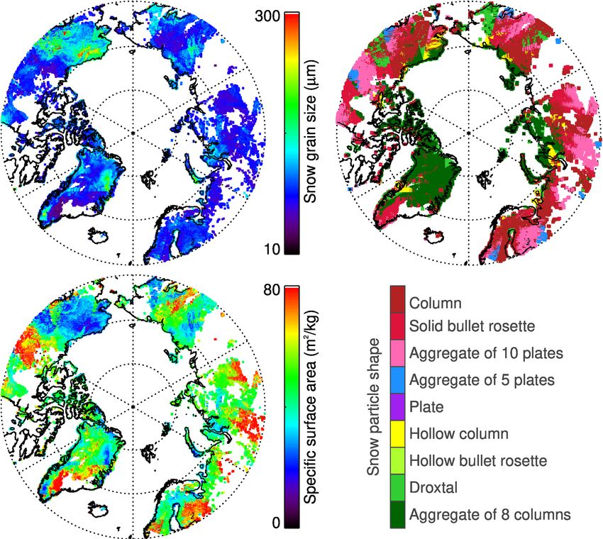
Figures 9 and 10 show the time series of SGS and SSA high spatial resolution. This might explain why the deviation
over each site. We can see that sites Greenland and Antarc- of the retrieved SGS values in this area are largest around
tica provide most of the match-ups. Both SGS and SSA 13:00 UTC when flight altitude was in the range of 100 m.
show good agreement between XBAER-derived and field- The SGS retrieval based on the algorithm suggested by
measured values over these two sites. For SGS, the correla- Zege et al. (2011) and Carlsen et al. (2017) gives the optical
tion coefficients are 0.85 and 0.89 and the RMSEs are 14 and radius of the snow grains such that the SSA can be derived
9 µm, respectively. For SSA, those values are 0.84 and 0.89 applying Eq. (A1) from the companion paper. The map of
for the correlation coefficient and 8 and 7 m2 /kg for RMSE, the SSA (Fig. 11c) reflects a similar pattern to that observed
respectively. Although the other sites provide limited match- for the SGS, showing an inverse behavior to that depicted
ups, they still give helpful information for the understanding in Fig. 11a. On average, XBAER (mean SSA 24 ± 3 m2 /kg)
of impacts of surface and atmospheric conditions. In gen- and SMART (mean SSA 21 ± 5 m2 /kg) agree within the 1σ
eral, sites China and Japan show large AOT values, leading to standard deviation. The correlation of SSA between XBAER
underestimation of SGS and overestimation of SSA. For the and SMART is similar to that for the SGS with a correlation
two Canadian sites (Canada-Alex, Canada-Josh), the under- coefficient R of 0.81 and RMSE of 2.0 m2 /kg. A comprehen-
/overestimation of SSA and SGS may largely be explained sive comparison between XBAER and SMART is given in
by the surface condition. The Alps site seems to be affected Jäkel et al. (2021).
by both surface and atmospheric impacts. Since XBAER is also designed to support the MOSAiC
campaign on an Arctic-wide scale (Mei et al., 2020c), it is
5.3 Validation using the observations of aircraft important to have an overview of how snow properties look
campaign on an Arctic-wide scale for the existing campaign. Figure 12
shows the SGS, SPS and SSA geographic distribution over
The optical snow grain size over Arctic sea ice was de- the whole Arctic for 26 March 2018. Northern Greenland,
rived from airborne SMART measurements as described in North America and central Russia show large snow particles,
Sect. 2.3. Figure 11a shows the retrieved grain size along the especially over North America. And the SPS shows more
flight track (black-encircled area) taken on 26 March 2018 diversity in lower latitudes compared to the central Arctic,
between 12:00 and 14:00 UTC north of Greenland. During indicating a stronger SPMP. An aggregated shape such as
this period of cloudless conditions, a Sentinel-3 overpass aggregate of 8 columns is the dominant shape in the cen-
(12:29 UTC) delivered SGS data based on the XBAER al- tral Arctic, while column is one of the dominant shapes in
gorithm as displayed in the background of this map with lower latitudes. SSA shows large values in the lower-latitude
a 1 km spatial resolution. In general, lower SGSs were ob- Arctic (northern Canada, southern Greenland, western Nor-
served by both methods in the vicinity of Greenland, while way, southern Finland, northern Russia), while the values are
in particular in the northeast region of the map (dashed red smaller in the central Arctic.
circle in Fig. 11a) SGS values of up to 350 µm were de-
rived from the aircraft albedo measurements. The XBAER
algorithm also reveals higher values in this region. For a di- 6 Discussion
rect comparison, XBAER data were allocated to the time se-
ries of the SMART measurements along the flight track. Af- The above analysis shows the promising quality of XBAER-
terwards all successive SMART data points assigned to the derived SGS, SPS and SSA results. The XBAER-retrieved
same XBAER location were averaged to compile a joint time SGS, SPS and SSA can be used to understand the change
series of both datasets as displayed in Fig. 11b. Overall a in snow properties temporally. Even though the snow meta-
correlation coefficient of R = 0.82 and an RMSE of 12.4 µm morphism depends on the environmental conditions, Aoki
were derived, where SMART (mean SGS 165 ± 40 µm) gen- et al. (2000) and Saito et al. (2019) pointed out that a 4 d
erally shows larger grain sizes than XBAER (mean SGS timescale is a reasonable time span to see the temporal
138 ± 21 µm). The course of the SGS follows a similar pat- change in snow properties. Figure 13 shows XBAER-derived
tern for both methods, with the largest deviations when the SGS (upper panels), SPS (middle panels) and SSA (lower
aircraft measured in the area depicted by a dashed red cir- panels) over Greenland during 27–30 July 2017. Large vari-
https://doi.org/10.5194/tc-15-2781-2021 The Cryosphere, 15, 2781–2802, 2021You can also read