Projections of shipping emissions and the related impact on air pollution and human health in the Nordic region
←
→
Page content transcription
If your browser does not render page correctly, please read the page content below
Atmos. Chem. Phys., 21, 12495–12519, 2021
https://doi.org/10.5194/acp-21-12495-2021
© Author(s) 2021. This work is distributed under
the Creative Commons Attribution 4.0 License.

Projections of shipping emissions and the related impact
on air pollution and human health in the Nordic region
Camilla Geels1,2 , Morten Winther1 , Camilla Andersson3 , Jukka-Pekka Jalkanen4 , Jørgen Brandt1,2 , Lise M. Frohn1,2 ,
Ulas Im1,2 , Wing Leung3 , and Jesper H. Christensen1,2
1 Department of Environmental Science, Aarhus University, Frederiksborgvej 399, P.O. Box 358, 4000 Roskilde, Denmark
2 iCLIMATE,  Interdisciplinary Centre for Climate Change at Aarhus University, Aarhus, Denmark
3 Swedish Meteorological and Hydrological Institute, 60176 Norrköping, Sweden
4 Atmospheric Composition Research, Finnish Meteorological Institute, P.O. Box 503, 00101 Helsinki, Finland

Correspondence: Camilla Geels (cag@envs.au.dk)

Received: 16 December 2020 – Discussion started: 9 February 2021
Revised: 22 June 2021 – Accepted: 5 July 2021 – Published: 19 August 2021

Abstract. International initiatives have successfully brought     within the Nordic region approximately 9900 persons died
down the emissions, and hence also the related negative im-       prematurely due to air pollution in 2015 (corresponding to
pacts on environment and human health, from shipping in           approximately 37 premature deaths for every 100 000 inhab-
Emission Control Areas (ECAs). However, the question re-          itants). When including the projected development in both
mains as to whether increased shipping in the future will         shipping and land-based emissions, this number is estimated
counteract these emission reductions. The overall goal of         to decrease to approximately 7900 in 2050. Shipping alone is
this study is to provide an up-to-date view on future ship        associated with about 850 premature deaths during present-
emissions and provide a holistic view on atmospheric pol-         day conditions (as a mean over the two models), decreasing
lutants and their contribution to air quality in the Nordic       to approximately 600 cases in the 2050 BAU scenario. In-
(and Arctic) area. The first step has been to set up new and      troducing a HFO ban has the potential to lower the number
detailed scenarios for the potential developments in global       of cases associated with emissions from shipping to approx-
shipping emissions, including different regulations and new       imately 550 in 2050, while the SECA scenario has a smaller
routes in the Arctic. The scenarios include a Baseline sce-       impact. The “worst-case” scenario of no additional regula-
nario and two additional SOx Emission Control Areas (SE-          tion of shipping emissions combined with a high growth in
CAs) and heavy fuel oil (HFO) ban scenarios. All three sce-       the shipping traffic will, on the other hand, lead to a small
narios are calculated in two variants involving Business-As-      increase in the relative impact of shipping, and the number
Usual (BAU) and High-Growth (HiG) traffic scenarios. Ad-          of premature deaths related to shipping is in that scenario
ditionally a Polar route scenario is included with new ship       projected to be around 900 in 2050. This scenario also leads
traffic routes in the future Arctic with less sea ice. This has   to increased deposition of nitrogen and black carbon in the
been combined with existing Current Legislation scenarios         Arctic, with potential impacts on environment and climate.
for the land-based emissions (ECLIPSE V5a) and used as
input for two Nordic chemistry transport models (DEHM
and MATCH). Thereby, the current (2015) and future (2030,
2050) air pollution levels and the contribution from ship-        1   Introduction
ping have been simulated for the Nordic and Arctic areas.
Population exposure and the number of premature deaths at-        The shipping sector plays a key role for tourism and the trans-
tributable to air pollution in the Nordic area have thereafter    portation of goods in Europe and beyond (EEA, 2017). Due
been assessed by using the health assessment model EVA            to the use of fossil fuels, shipping activities lead to emissions
(Economic Valuation of Air pollution). It is estimated that       of important air pollutants like nitrogen oxides (NOx ), sul-
                                                                  fur dioxide (SO2 ), primary particles with a diameter of less

Published by Copernicus Publications on behalf of the European Geosciences Union.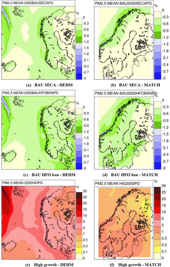
12496      C. Geels et al.: Projections of shipping emissions and the related impact on air pollution in the Nordic region

than 2.5 µm (PPM2.5 ) and black carbon (BC). The many neg-        the western part of the Mediterranean (up to 45 %) and along
ative impacts related to these air pollutants and compounds       the northern European coast (10 %–15 %). However, a signif-
subsequently formed in the atmosphere are well established.       icant contribution from ships to air quality was also reported
Nitrogen deposition is a threat to sensitive ecosystems, and      in Madrid area, Spain, despite the inland location of the city
increasing deposition is associated with loss of biodiversity     (Nunes et al., 2020). A health assessment for eight European
(Bobbink et al., 2010), while compounds such as ozone (O3 ),      Mediterranean coastal cities found that shipping emissions
nitrogen dioxide (NO2 ) and fine particulate matter (PM2.5 )      can be related to about 5.5 premature deaths per year for ev-
are known to have negative impacts on human health (as re-        ery 100 000 inhabitants in the eight cities (Viana et al., 2020).
viewed in, e.g. WHO, 2013; Pope et al., 2020), even in the           In the Arctic, shipping can also be an important source
Nordic area where there are relatively low exposure levels        for pollution in an otherwise clean and pristine environment
(Raaschou-Nielsen et al., 2020). Components like BC are           (Schmale et al., 2018). With decreasing sea ice extent in a
also very important in relation to the climate system (Bond       warming Arctic, new trans-Arctic shipping routes are becom-
et al., 2013) and lead to warming, especially in the Arctic re-   ing more likely (Corbett et al., 2010), and this can increase
gion (AMAP, 2011). In recognition of the negative impacts,        the traffic in the area and add to the air pollution levels in the
sulfur emissions from ships have been regulated by establish-     high Arctic (Winther et al., 2014, 2017).
ing Sulfur Emission Control Areas (SECAs) for the Baltic             In the current study, we take on a Nordic perspective in or-
and North seas, as well as close to the North American coast-     der to make an updated analyses of future shipping emissions
line and Puerto Rico. In addition to these regional reductions,   and the impacts these emissions have on health and environ-
a global shift to low-sulfur fuels was required from 2020 on-     ment. We have the following two overall aims.
wards. This reduction was decided by the Marine Environ-
                                                                    1. We aim to set up shipping emission scenarios that in-
ment Protection Committee under the International Maritime
                                                                       clude several options to limit ship emissions, ranging
Organization in 2016, considering the health and climate im-
                                                                       from additional fuel quality requirements (Heavy fuel
pact of reducing sulfur emissions (Sofiev et al., 2018). Fur-
                                                                       Oil ban), which go beyond the already agreed global
ther, a NOx Emission Control Area (NECA) was established
                                                                       sulfur cap, and an expansion of the existing ECA ar-
for North America, and new ships built after 2016 will need
                                                                       eas. Thus, the scenarios include a Baseline scenario and
to comply with IMO Tier III emission requirements, which
                                                                       two additional SOx Emission Control Area (SECA) and
will reduce NOx emissions from these ships by 80 % when
                                                                       heavy fuel oil (HFO) ban scenarios. All three scenarios
compared to Tier I level. Similar rules will be applied to the
                                                                       are calculated in two variants involving Business-As-
Baltic Sea and North Sea areas from 2021 onwards. Ship-
                                                                       Usual (BAU) and High-Growth (HiG) traffic scenarios
ping activity is nevertheless predicted to increase (e.g. Cor-
                                                                       and an additional Polar route scenario is also included,
bett et al., 2010), and the global Fourth IMO Greenhouse Gas
                                                                       which includes new ship traffic routes due to less Arctic
(GHG) study (Faber et al., 2020) projects a strong growth
                                                                       sea ice in the future. The work reported here is based on
up to 2050, with GHG emission levels ranging from 90 %–
                                                                       vessel-level modelling of ship emissions using realistic
150 % of 2008 levels regardless of the measures currently in
                                                                       traffic data to describe the spatio-temporal variation of
force.
                                                                       traffic patterns.
   According to a recent study of Sofiev et al. (2018), ship-
ping is responsible for about 266 000 premature deaths glob-        2. We also aim to assess the contribution from shipping
ally, even after the 2020 sulfur reduction is implemented.             emissions to air pollution in the Nordic and Arctic area
This reduction is estimated to decrease the human health               and the potential benefits of the mitigation options in-
effects by 137 000 deaths, especially in Asia and India but            cluded in the shipping emission scenarios. This is done
to a significantly lower extent in the Northern Hemisphere,            by applying two chemical transport models (DEHM and
where sulfur emissions are already regulated by existing SE-           MATCH) set up with land-based and shipping emis-
CAs. For Europe, an earlier study estimated that up to 50 000          sions and analysing maps of the modelled air pollu-
premature deaths per year can be associated with emissions             tion concentrations resulting from all emissions and the
from shipping (Brandt et al., 2013b). More recently, a study           share related to shipping. It is expected that models with
zoomed in on the Baltic Sea region and estimated that Baltic           different physical descriptions and setups show some
PM2.5 emissions from shipping caused up to 2300 premature              differences in modelled air pollution, and by using two
deaths in the surrounding countries in 2016, which was a re-           models an indication of the related uncertainties is dis-
duction of 37 % compared to before a SECA was enforced in              played. The included emissions represent present-day
the Baltic (Barregard et al., 2019). Overall, the impacts will         conditions and future projections towards 2050. For the
be largest in coastal areas, and a review has previously found         Nordic area, we focus mainly on total PM2.5 (the sum of
that shipping emissions contribute to 1 %–14 % of the PM2.5            primary emitted components, e.g. black carbon and sec-
levels and 7 %–24 % of the NO2 levels in coastal areas in Eu-          ondary formed aerosols), while for the Arctic we focus
rope (Viana et al., 2014). Aksoyoglu et al. (2016) found the           on the deposition of nitrogen and black carbon. Further-
contribution from shipping to the total PM2.5 to be largest in         more, the modelled concentration maps serve as input

Atmos. Chem. Phys., 21, 12495–12519, 2021                                          https://doi.org/10.5194/acp-21-12495-2021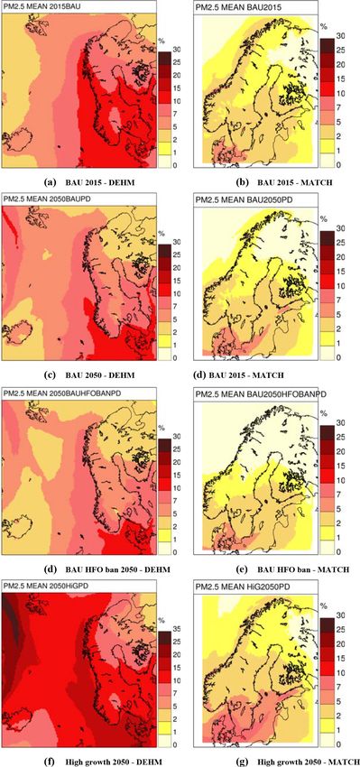
C. Geels et al.: Projections of shipping emissions and the related impact on air pollution in the Nordic region           12497

       to the health impact assessment system EVA (Economic       2.1.2   Traffic activity data in the DCE ship emission
       Valuation of Air pollution) in order to assess the over-           model
       all impacts of air pollution on the human health in the
       Nordic area and the changes in health impacts resulting    The ship activity data used in the DCE ship emission model
       from the different ship emission scenarios. The focus      are provided by the Danish Maritime Authority (DMA)
       here is on mortality and the number of premature deaths    based on AIS signals received from terrestrial base stations
       associated with exposure to air pollution.                 and from satellites equipped with AIS receivers for the area
                                                                  north of 60◦ N. The data represent the years 2012–2016, di-
                                                                  vided into 0.5◦ longitude × 0.225◦ latitude grid cells with a
2     Materials and methods                                       monthly resolution. The ships are classified into 14 ship types
                                                                  and 16 ship length categories, and data for total sailed dis-
2.1     Setup of shipping emission inventories
                                                                  tance and average sailing speeds are provided stratified into
The background data for the emission scenarios is traffic data    the different ship type–length–average speed combinations
for the area north of 60◦ N, emission factors, and scenario-      that have been recorded in the individual cells.
specific emission inventories from the ship emission model           A weighted and consolidated ship activity data set for a
developed at the Danish Centre for Environment and En-            base year was prepared for the DCE ship emission model
ergy (DCE) at Aarhus University (Winther et al., 2017). In        based on the 5-year ship activity data provided by DMA in
order to obtain a spatial coverage of the entire Nordic area      order to avoid inexpedient temporal and spatial specific fluc-
and the Arctic, the DCE emission inventories are combined         tuations in traffic records and in order to achieve a uniform
with a global CO2 ship emission inventory produced with           grid cell reference system for the emission projection calcu-
the Ship Traffic Emissions Assessment Model (STEAM) for           lations.
2015 (Johansson et al., 2017).                                       The traffic scaling factors used in the DCE ship emission
                                                                  model for traffic projections are derived from traffic growth
2.1.1    STEAM model                                              factors in the Corbett et al. (2010) Business-As-Usual (BAU)
                                                                  and High-Growth (HiG) scenarios by referring the DCE ship
Global emission data from the STEAM model (developed at           types to the Corbett et al. (2010) ship types and by using Cor-
the Finnish Meteorological Institute) from an earlier study       bett traffic growth factors evolved from the base year. Fuel
(Johansson et al., 2017) were applied in this work. The           efficiency improvements for future ships are modelled from
model uses global Automatic Identification System (AIS)           EEDI fuel efficiency regulations agreed by Marpol 83/78 An-
data to describe shipping activity and it applies vessel-level    nex VI and mandatory from 1 January 2013 for newly built
modelling using technical descriptions of each ship in the        ships larger than 400 GT. For further explanations regarding
global fleet (Jalkanen et al., 2009, 2012; Johansson et al.,      ship activity data, traffic scaling factors and EEDI factors,
2013, 2017). Details of the method and the numerical re-          see Winther et al. (2017).
sults for emissions used in this study can be found in Johans-
son et al. (2017). The AIS data from terrestrial and satel-       2.1.3   Scenarios
lite networks were purchased from Orbcomm Ltd. (Rochelle
Park, USA), and the technical details database was acquired       The current study includes a Baseline emission projection
from IHS Markit (IHS Markit Global Headquarters, fourth           scenario and two additional emission projections: a SECA
floor Ropemaker Place, 25 Ropemaker Street, London EC2Y           (Sulfur Emission Control Area) scenario and an HFO (heavy
9LY, UK). Emissions for ships were modelled without con-          fuel oil) ban scenario (see Table 1). The Baseline scenario
sidering weather effects (wind, waves, ice, currents) and thus    forms the basis for the SECA and HFO ban scenarios.
represent ideal conditions, which may introduce uncertain-           All three scenarios use the BAU and HiG traffic activity
ties when compared to real emissions and fuel consump-            projections explained above in Sect. 2.1.2, and the scenarios
tion. Regardless, average absolute deviation of the STEAM-        further assume an increasing amount of liquefied natural gas
predicted fuel consumption for any single ship is around          (LNG) fuel being used as a substitution for heavy fuel oil
19 %, whereas inventory-level totals are equivalent to those      in the inventory area throughout the projection years. The
reported in the EU Monitoring, Reporting and Verification         scenarios use the “low case” LNG fuel share of total marine
system (EU, 2015). These comparisons were made for more           fuel consumption, which is 2 %, 4 % and 8 % in the years
than 2550 vessels reporting their fuel consumption during the     2020, 2030 and 2050, respectively, as described in the IMO
reporting year 2019.                                              third GHG study published by IMO (2015).
                                                                     The Baseline scenario assumes an increase in the use
                                                                  of exhaust gas cleaning systems (EGCS) for SO2 emission
                                                                  abatement in the case of ships using HFO with a high content
                                                                  of sulfur. In the Baseline scenario inside the existing SECA
                                                                  zones (i.e. American, North Sea and Baltic Sea SECAs), the

https://doi.org/10.5194/acp-21-12495-2021                                       Atmos. Chem. Phys., 21, 12495–12519, 2021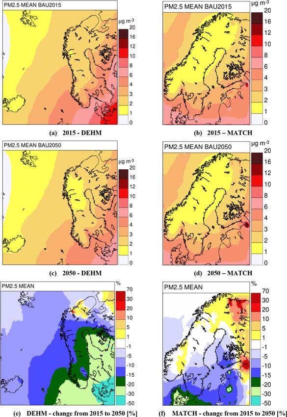
12498      C. Geels et al.: Projections of shipping emissions and the related impact on air pollution in the Nordic region

Table 1. Total shipping emissions for the Nordic (d03) domain for the base year 2015; the Baseline, SECA, and HFO ban BAU scenarios in
2020, 2030, and 2050; and percent changes between Baseline and SECA/HFO ban scenario results in 2020, 2030, and 2050.

                                                              BAU                                   HiG
                          Scenario     Year    Fuel   CO2     SO2     NOx     BC     Fuel   CO2     SO2    NOx      BC
                                                Mt     Mt      Kt      Kt      Kt     Mt     Mt      Kt     Kt       Kt
              Total       Base year    2015     9.6    30.3   59.6    719    0.80     9.6   30.3    59.6    719    0.80
                          Baseline     2020    10.2    32.1   23.4    739    0.75    10.7   33.9    24.7    781    0.79
                                       2030    10.9    34.3   24.1    574    0.81    12.5   39.2    27.5    661    0.93
                                       2050    13.3    41.6   27.2    292    0.97    18.3   57.0    37.5    400    1.35
              % change    SECA         2020       0       0   −31        0    −2        0      0    −31        0    −2
                                       2030       0       0   −29        0    −2        0      0    −29        0    −2
                                       2050       0       0   −27        0    −1        0      0    −27        0    −1
                          HFO ban      2020       0       0   −33        0    −9        0      0    −33        0    −9
                                       2030       0       0   −32        0   −12        0      0    −32        0   −13
                                       2050       0       0   −31        0   −16        0      0    −31        0   −17

fuel type switches from HFO to marine diesel and marine              2.45 % HFO is used with a removal efficiency equivalent to
gas oil (MDO/MGO) for ships using HFO that do not have               Fs = 0.1 %. EGCS systems are included in the emission pro-
an EGCS installed (Winther et al., 2017). Outside the exist-         jections from 2020 onwards (Sect. 2.2.3). For MDO/MGO,
ing SECAs, the latter ships use 0.5 % HFO after the global           Fs equals 0.08 %, as monitored by IMO (2016).
sulfur cap introduction in 2020.                                        The BC emission factors used in this project are measured
   In the SECA scenario, the existing SECA zones (i.e.               values by Aakko-Saksa et al. (2016). The BC emission fac-
American, North Sea and Baltic Sea SECAs) are expanded               tors for 2.45 % HFO, 0.5 % HFO and MDO/MGO are 0.155,
to cover the entire inventory area. The SECA scenario takes          0.065 and 0.056 g kg−1 fuel, respectively. For HFO-fuelled
into account the Baseline shares of LNG fuel consumption             ships with EGCS, an average BC removal efficiency of 40 %
and EGCS installations. Further into the SECA scenario, the          is assumed (i.e. 0.093 g kg−1 fuel) based on the available data
fuel shifts from HFO to MDO/MGO outside the existing SE-             from the literature (ICCT, 2015; Lack and Corbett, 2012;
CAs to ships using HFO and not using EGCS.                           Johnson et al., 2016). For LNG, a BC emission factor of
   In the HFO ban scenario, no use of HFO by ships is al-            0.00155 g kg−1 fuel is used, derived as 1 % of the BC emis-
lowed at all in the inventory area. The HFO ban scenario             sions for HFO (ICCT, 2015).
includes the consumption of LNG as assumed in the Base-                 The full set of basis emission factors is not shown here,
line scenario. The remaining part of the HFO consump-                but they are explained in more detail in Winther et al. (2017).
tion not being substituted by LNG is assumed to switch to            However, aggregated from ship type, engine type, fuel type
MDO/MGO in the entire inventory area.                                and engine production year, fuel-related emission factors for
                                                                     2015 and the forecast years 2020, 2030 and 2050 are shown
2.1.4   Emission factors                                             in Fig. S1 in the Supplement that have been derived from the
                                                                     fuel and emission results presented above. The development
The specific fuel consumption factors (SFCs) and NOx emis-           of the emission factors reflects the emission technology im-
sion factors (g kWh−1 ) for HFO and MDO/MGO used in                  provements (for NOx ) and fuel sulfur content and the Base-
the calculations are classified according to engine type and         line shares of LNG fuel consumption and EGCS installations
engine production year (Ministry of Transport, 2015; MAN             (for SO2 and BC). The emission factors applied (Fig. S1) in-
Energy Solutions, 2012). The CO2 emission factors (g kg−1            clude the emission factor adjustments made in the calcula-
fuel) come from Nielsen et al. (2019). For LNG, the source           tions in order to account for engine load variations (Winther
of SFCs, NOx and CO2 emission factors is IMO (2015).                 et al., 2017).
   The SO2 emission factors are proportional with the fuel
sulfur content (Fs), or the sulfur removal efficiency in             2.1.5   Scaling of the global CO2 ship emission inventory
cases regarding ships with EGCS installed. For HFO-fuelled
ships without EGCS installed, Fs corresponds to the global           In order to cover the entire Nordic area and the Arctic and
IMO monitoring value of 2.45 % for 2015 (IMO, 2016)                  make use of already well-defined and elaborated scenarios
and the global fuel sulfur cap of 0.5 % for 2020 onwards.            for shipping in the Arctic, the global CO2 ship emission in-
For HFO-fuelled ships with EGCS installed, by assumption             ventory produced with the STEAM model for 2015 is used

Atmos. Chem. Phys., 21, 12495–12519, 2021                                             https://doi.org/10.5194/acp-21-12495-2021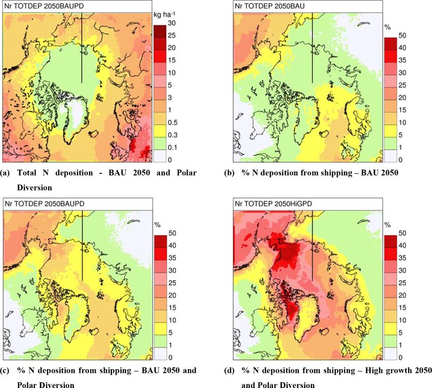
C. Geels et al.: Projections of shipping emissions and the related impact on air pollution in the Nordic region             12499

                                                                   istry transport model (CTM) originally developed in the early
                                                                   1990s to study the atmospheric transport of sulfur dioxide
                                                                   and sulfate into the Arctic (Christensen, 1997). The model
                                                                   has been modified, extended and updated continuously since
                                                                   then and now includes a comprehensive chemical scheme,
                                                                   detailing 80 chemical species and 158 chemical reactions, in-
                                                                   cluding a Volatile Basis Set (VBS) for describing secondary
                                                                   organic aerosols (SOA) (see, e.g. Brandt et al., 2012, for a de-
                                                                   tailed description of DEHM, and Bergstrøm et al., 2012, for a
                                                                   description of the VBS part). In the current study, DEHM has
                                                                   been set up with a main domain covering the Northern Hemi-
                                                                   sphere and part of the Southern Hemisphere and a resolution
                                                                   of 150 km × 150 km. Within this domain, a nested domain
                                                                   (d02) with a resolution of 50 km × 50 km covers the Arctic
                                                                   and Europe and a second nested domain (d03) with a reso-
                                                                   lution of 16.67 km × 16.67 km covers the Nordic region (see
                                                                   Fig. 1).
                                                                      The meteorological data driving DEHM are calculated us-
                                                                   ing the WRF model (Skamarock et al., 2008), set up with
                                                                   the same domains and nests as DEHM, and forced with
Figure 1. The study area as defined by the three domains used in   ERA-Interim meteorology (Dee et al., 2011). Natural emis-
the DEHM model (d01–d03) and the domain used in the MATCH
                                                                   sions like sea salt and biogenic volatile organic compounds
model (m).
                                                                   (VOCs) are calculated online in the model as a function
                                                                   of meteorological parameters (described in Soares et al.,
in combination with the Arctic fuel consumption and emis-          2016; Zare et al., 2012, 2014). The anthropogenic emis-
sion scenarios calculated with the DCE ship emission model         sions for the current and future periods are based on the
for 2015, 2020, 2030 and 2050 (Winther et al., 2017). The          global 0.5◦ × 0.5◦ ECLIPSE V5a data sets including sec-
STEAM data stops at 74◦ N, and thus the area beyond this is        toral emissions (https://www.iiasa.ac.at/web/home/research/
covered by the DCE model.                                          researchPrograms/air/Global_emissions.html, last access:
   The ship types defined in the DCE ship emission model are       16 July 2015). We apply the future Baseline scenario assum-
mapped into the ship types defined in the STEAM model.             ing current legislation (CLE) for the air pollution compo-
Subsequently, the STEAM 2015 CO2 emission results per              nents (see Klimont et al., 2017, for an overview). The pro-
ship type, together with aggregated fuel-related CO2 emis-         jected changes in the land-based emissions in the applied do-
sion factors per ship type for 2015 derived from the DCE           mains in DEHM are given in Table S1 in the Supplement.
model, are used to calculate fuel consumption results spe-         The shipping emissions in ECLIPSE V5a have been replaced
cific for each ship type. A spatial distinction is made between    with the new shipping emissions described in Sect. 2.1. We
SECA and non-SECA sea areas in the calculations.                   have run the model for the meteorological year 2015 (with
   In each of the scenarios, for a given scenario year and ship    December 2014 as spin up) with a combination of land-
type, the percentage change in total fuel consumption ob-          based ECLIPSE V5a and new shipping emissions represent-
tained with the DCE model from 2015 to the scenario year           ing the years 2015, 2030 and 2050. This is done in order
is then used to scale the 2015 STEAM model fuel consump-           to isolate the impact from emission changes. Additionally,
tion, in order to calculate STEAM-related fuel consumption         we have made simulations with and without a new polar di-
results for the scenario year in question.                         version route and simulations where the shipping emissions
   STEAM-related emission results are subsequently ob-             have been reduced by 30 % (i.e. multiplied by 0.7). By scal-
tained as the product of (1) the aggregated emission factors       ing the results afterwards, the impact from shipping alone
obtained with the DCE ship emission model for each sce-            can be analysed, but non-linear effects of atmospheric chem-
nario, scenario year, and STEAM ship type and (2) the cor-         istry are still included. In total, 22 simulations have been
responding fuel consumption. The final emission data set for       made with the DEHM model (an overview of model runs is
2015 and the scenario years are monthly files with a spatial       given in Table S2 in the Supplement). The Baseline simula-
resolution of 0.1◦ × 0.1◦ .                                        tion with 2015 BAU emissions has been evaluated by com-
                                                                   parison to European observations of the components relevant
2.2   The DEHM model                                               for the health assessment (PM2.5 , NO2 and O3 ), and a suf-
                                                                   ficiently good agreement between model and observations
The Danish Eulerian Hemispheric Model (DEHM) is a state-           is seen both in terms of level (fractional bias for daily val-
of-the-art three-dimensional, Eulerian, atmospheric chem-          ues in 2015: −0.09, 0.03 and 0.05 for PM2.5 , NO2 , and O3 )

https://doi.org/10.5194/acp-21-12495-2021                                        Atmos. Chem. Phys., 21, 12495–12519, 2021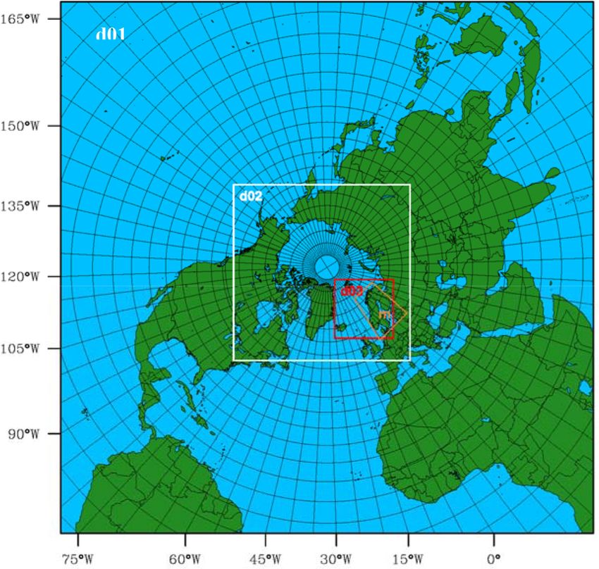
12500     C. Geels et al.: Projections of shipping emissions and the related impact on air pollution in the Nordic region

and variability (correlations for daily values in 2015: 0.79,    lation coefficients of daily mean PM10 , PM2.5 , O3 and NO2
0.73 and 0.93; see the Supplement for details). Furthermore,     are −11 %/0.59, −13 %/0.67, 1.6 %/0.70 and −5.9 %/0.58,
the DEHM model is one of the core models in the Coper-           respectively). An evaluation of MATCH for the Fennoscan-
nicus Atmosphere Monitoring Service (CAMS) providing             dia region for the year 2015 is included in the Supplement
daily air pollution forecasts and analyses, which are contin-    of this paper. MATCH is also a core model in the opera-
uously evaluated online against European observations (see       tional CAMS (Marécal et al., 2015; https://www.regional.
https://www.regional.atmosphere.copernicus.eu/, last access:     atmosphere.copernicus.eu/, last access: 16 December 2020)
16 December 2020).                                               and includes daily updates of daily air pollution forecasts,
   The study area and the included model domains are shown       fused measurement and modelling of atmospheric concen-
in Fig. 1.                                                       trations (through data assimilation), as well as model perfor-
                                                                 mance scores. MATCH is a building block in the MATCH
2.3   The MATCH model                                            Sweden system for environmental surveillance (Andersson
                                                                 et al., 2017) and includes measurement model fusion of to-
The MATCH (Multi-scale Atmospheric Transport and                 tal atmospheric deposition (MMF-TDEP) of ozone, nitrogen,
CHemistry) model (Robertson et al., 1999; Andersson et al.,      sulfur and base cations.
2007, 2015) is a state-of-the-art Eulerian chemistry and
transport model, including wet, thermal and photochemical        2.4   The EVA system
reactions, to describe the sulfur and nitrogen cycle, tropo-
spheric ozone chemistry, and particle formation and transfor-    The EVA (Economic Valuation of Air pollution; Brandt et al.,
mation. The version used in the current set up is the same as    2013a, b; Geels et al., 2015, Im et al., 2018) model system is
was used in the EURODELTA-Trends exercise (Colette et al.,       based on the impact pathway chain (Friedrich and Bickel,
2017). It includes online emissions of sea salt as described     2001), wherein modelled air pollution levels are coupled to
in Soares et al. (2016). Secondary organic aerosol formation     population data for calculation of human exposure, health
is modelled through a volatility basis set, and biogenic VOC     impacts (both mortality and morbidity) and related exter-
emissions are modelled online, both as described by Simpson      nal costs. In the current study, we focus on the health im-
et al. (2012). Further details on the model configuration are    pacts and do not include the assessment of the cost. The
described in Colette et al. (2017). The driving meteorological   health impacts are calculated using linear exposure–response
forcing data used was the HIRLAM operational weather data        functions, which in the applied model version (EVAv5.2) are
for 2015 for the domain covering Fennoscandia (11 km res-        based on the HRAPIE recommendations (WHO, 2013). The
olution). The lateral and top boundaries of this domain were     number of premature deaths in the system is calculated from
fed every 6 h by results from the DEHM model, i.e. domain        short-term exposure to O3 , NO2 , SO2 and PM2.5 , as well as
d01 (see Fig. 1). The anthropogenic and shipping emissions       long-term exposure to PM2.5 and NO2 . The EVA model sys-
were the same as for DEHM, but with MATCH we simulate            tem can be used to estimate the health impacts due to the
the current scenario (2015) and a selection of 2050 shipping     total air pollution levels or due to contributions from various
scenarios. The MATCH grid is smaller than the DEHM d03           model scenario runs, where, e.g. specific emission sectors are
grid with a finer horizontal resolution (11 km × 11 km). The     reduced or the weather and climate scenarios are changed. In
shipping attribution was conducted in the same manner as         this study, the population exposure has been assessed for the
with the DEHM model, i.e. by reducing the shipping emis-         d03 DEHM domain by combining the concentration maps
sions by 30 % and using the corresponding DEHM simula-           from both DEHM and MATCH with gridded population data
tion on the boundary of the MATCH grid. In total, 12 simu-       from EUROSTAT for 2015 (see Table S4) with the national
lations have been made with the MATCH model (Table S2 in         total populations and a map (Fig. S5) of the population dis-
the Supplement).                                                 tribution in the applied 16.67 km × 16.67 km grid). In order
   The current model configuration is extensively evaluated      to do so, the MATCH 11 km × 11 km gridded data have been
with in situ observations and compared to the performance        aggregated to the d03 grid. The EVA model system has been
of other models in numerous papers in similar setups as in       compared to other similar models (Anenberg et al., 2015;
this study for ozone, particles and nitrogen and sulfur depo-    Lehtomäki et al., 2020), is part of the Danish monitoring
sition in Europe (Otero et al., 2018; Theobald et al., 2019;     programme (Ellermann et al., 2020) and has been used rou-
Vivanco et al., 2018, Ciarelli et al., 2019a, b). The conclu-    tinely in numerous advisory projects for public authorities.
sion is that MATCH in the current configuration performs         In Sect. 3.2 the current results for 2015 are compared with
among the best models for near-surface ozone, as well as         EEA’s results for the same year (EEA, 2018).
nitrogen and sulfur deposition, and for particles it displays
high correlation with observations (fractional bias of daily
mean O3 , and correlation coefficients are 6 % and 0.80 in
Scandinavia in 2015), while PM concentrations are some-
what underestimated (for Europe fractional bias and corre-

Atmos. Chem. Phys., 21, 12495–12519, 2021                                        https://doi.org/10.5194/acp-21-12495-2021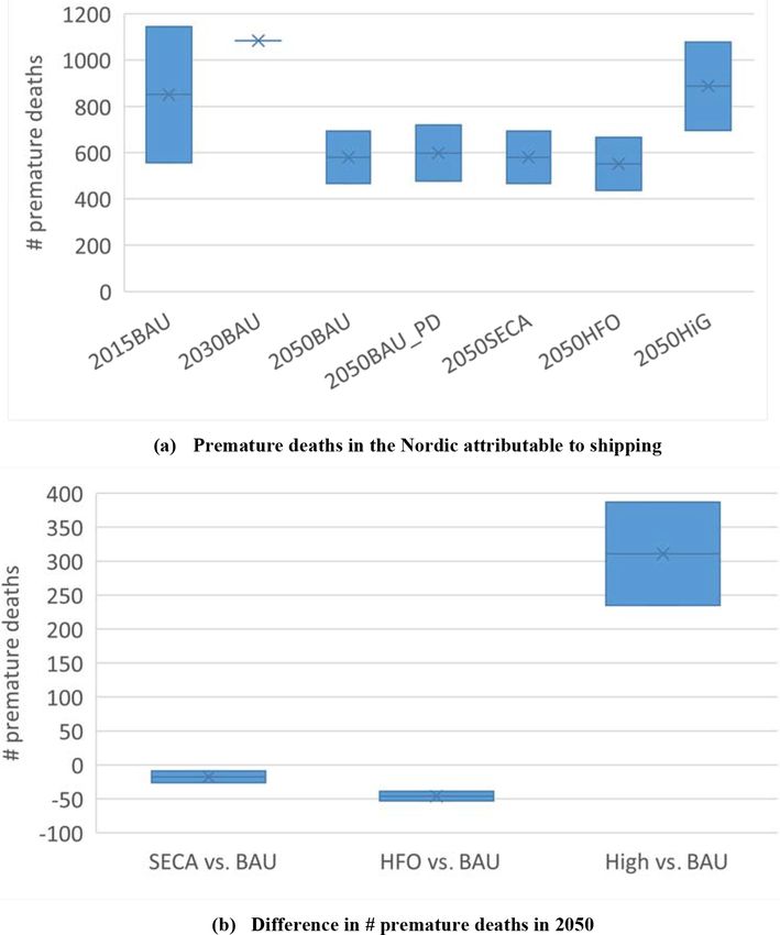
C. Geels et al.: Projections of shipping emissions and the related impact on air pollution in the Nordic region                  12501

Figure 2. CO2 , NOx , SO2 and BC emissions for 2015 and Baseline scenario results for 2020, 2030 and 2050, which have been further split
into SECA and non-SECA parts of domain d03.

3     Results                                                         3.1.1   Baseline results

In this section we first describe the projected developments          The emission development relies on the development in fuel
in the shipping emissions in the different scenarios within the       consumption and the corresponding emission factors. Fig-
Nordic area. Thereafter we describe the modelled present-             ure 2 shows the emissions of CO2 , NOx , SO2 and BC for
day air pollution levels with a focus on total PM2.5 and the          2015 and Baseline scenario results for 2020, 2030 and 2050,
overall health impact related to air pollution in the Nordic          which have been further split into the current ECA and non-
area. We then move on to the future developments in PM2.5             ECA parts of domain d03.
levels as simulated by the two models based on the shipping              In terms of total fuel consumption, the projected growth in
scenarios and the projected development of land-based emis-           ship traffic during the forecast period more than outweighs
sions. The related impacts on the number of premature deaths          the future fuel efficiency improvements for ships. From 2015
are then analysed. Next we focus more directly on the contri-         to 2050, the fuel consumption changes for total [SECA, non-
butions from shipping in terms of the PM2.5 levels and health         SECA] becomes 39 % [43 %, 20 %] for BAU traffic and 91 %
impacts. Finally we move to the Arctic and demonstrate how            [98 %, 51 %] for HiG traffic, respectively. Almost identical
the deposition of BC and nitrogen will be affected by the             percentage changes are calculated for CO2 emissions from
projected developments in emissions.                                  2015 to 2050 due to the almost constant fuel-dependent emis-
                                                                      sion factors for CO2 in the projection period (Fig. S1).
3.1    Development in shipping emissions                                 For NOx the Total [NECA, non-NECA] emission changes
                                                                      from 2015 to 2050 are −59 % [−70 %, 1 %] for BAU traf-
Table 1 shows the shipping emissions for the domain area              fic and −44 % [−58 %, 30 %] for HiG traffic, respectively.
d03 for the base year 2015 and the Baseline, SECA and HFO             The total NOx emission reductions during the forecast period
ban BAU scenarios in 2020, 2030 and 2050. The percent                 are due to the decrease in NOx emission factors (Fig. S1).
changes between Baseline and SECA and HFO ban scenario                NOx emission reductions are most significant for the exist-
results in 2020, 2030 and 2050 are also shown in Table 1.             ing NECA area, where new engines installed on ships from
                                                                      1 January 2021 must comply with the most stringent IMO
                                                                      Tier III NOx emission standards.

https://doi.org/10.5194/acp-21-12495-2021                                            Atmos. Chem. Phys., 21, 12495–12519, 2021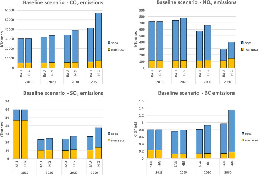
12502      C. Geels et al.: Projections of shipping emissions and the related impact on air pollution in the Nordic region

Figure 3. Emissions for domain d03 calculated in the Baseline, SECA and HFO ban BAU scenarios (CO2 , NOx , SO2 and BC) and the HiG
scenarios (SO2 and BC).

   The Total [SECA, non-SECA] SO2 emission changes                    Inside SECA, the emissions of BC increase somewhat
from 2015 to 2050 are −54 % [32 %, −78 %] for BAU traffic          more than what is expected from the changes in fuel con-
and −37 % [86 %, −71 %] for HiG traffic, respectively. For         sumption due to higher BC emission factors for HFO in com-
BC, the Total [SECA, non-SECA] emission changes from               bination with EGCS compared with the emission factors for
2015 to 2050 become 21 % [45 %, −39 %] for BAU traffic             the MDO/MGO fuel being replaced. The SO2 emissions in-
and 69 % [105 %, −22 %] for HiG traffic, respectively.             crease slightly less than fuel consumption due to the gradu-
   For SO2 and BC, the major reason for the emission re-           ally increased consumption of liquefied natural gas (LNG) in
ductions outside SECA from 2015 to 2050 is the shift from          the Baseline scenario.
HFO with a sulfur content of 2.45 % in 2015 to HFO with
0.5 % sulfur from 2020 onwards and the consequently re-            3.1.2   Emission and fuel consumption results across
duced emission factors. Compared with the HFO 2.45 % sul-                  scenarios
fur fuel, the less heavy 0.5 % sulfur fuel has a smaller amount
of heavy organic compounds; hence, the fuel combustion be-         The fuel consumption and NOx emission totals calculated for
comes more complete and BC emission factors consequently           the SECA and HFO ban scenario equal the results obtained
lower.                                                             in the Baseline scenario (Table 1; Fig. 3, NOx ). The main
                                                                   reason for this is that the engine-specific fuel consumption

Atmos. Chem. Phys., 21, 12495–12519, 2021                                          https://doi.org/10.5194/acp-21-12495-2021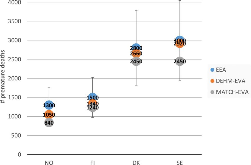
C. Geels et al.: Projections of shipping emissions and the related impact on air pollution in the Nordic region                12503

and NOx emission factors are unaffected by the fuel switch              line scenario for HiG traffic are calculated as the product of
from HFO to MDO/MGO, and the same shares of LNG of                      the diversion route fuel consumption and the emission factors
total fuel consumption per forecast year are also assumed in            derived from each of the four scenarios.
both scenarios (scenario definitions). Very small CO2 emis-                Table 2 shows the estimated emissions of CO2 , SO2 , NOx
sion differences between the Baseline, SECA and HFO ban                 and BC for the polar diversion routes passing through do-
scenarios are the result of small differences in the fuel-related       main d03 in 2020, 2030 and 2050 for the Baseline, SECA
CO2 emission factors for HFO and MDO/MGO.                               and HFO ban emission scenarios based on the BAU traffic
   In all scenario years for SO2 , the calculated emissions for         scenario and the Baseline emission scenario based on the
the SECA and HFO ban scenarios are close to 30 % lower                  HiG traffic scenario. The diversion emission results are also
than the emissions calculated for the Baseline scenario (Ta-            shown in Fig. S2 in the Supplement with the totals that do
ble 1). In the SECA scenario, HFO is only used by ships with            not include the diversion emission contribution (Table 1) for
EGCS, with a sulfur removal efficiency equivalent Fs = 0.1              each scenario case.
(Sect. 2.1.3). The 0.5 % fuel oil used outside the original                Based on the BAU diversion traffic scenarios for the fore-
SECA area, which is not being replaced by LNG, is replaced              cast years 2020 [2030, 2050], the additional percentage of
by MDO/MGO (Fs = 0.08) according to the scenario defi-                  emissions from ship traffic following the Arctic diversion
nitions. In the HFO ban scenario, all HFO consumption by                routes in all three scenarios is +3 % [+3 %, +9 %] for
ships not being replaced by LNG is replaced by MGO/MDO.                 CO2 and BC, +3 % [+4 %, +16 %] for NOx , +6 % [+6 %,
   For BC in 2020 [2030, 2050], the SECA scenario emis-                 +18 %] for SO2 (Baseline) and +3 % [+3 %, +9 %] for SO2
sions are 2 % [2 %, 1 %] lower than the Baseline results (Ta-           (SECA and HFO ban).
ble 1) in both traffic growth cases. For the HFO ban sce-                  The additional percentage of emissions from ship traf-
nario in 2020 [2030, 2050] with BAU traffic scenario, the               fic on Arctic diversion routes based on HiG diversion traf-
BC emissions are 9 % [12 %, 16 %] smaller than the Baseline             fic for the forecast years 2020 [2030, 2050] becomes +4 %
results (Table 1). For HiG traffic, the BC emissions become             [+8 %, +33 %] for CO2 , +4 % [+8 %, +33 %] for BC,
9 % [13 %, 17 %] smaller than the Baseline results.                     +7 % [+16 %, +65,%] for SO2 and +4 % [+10 %, +62 %]
   Apart from LNG with similar fuel consumption shares as-              for NOx .
sumed in all three scenarios, in the HFO ban scenario, only
the fuel type MDO/MGO with the smallest BC emission fac-                3.2   Present-day Nordic air pollution and health effects
tor (0.053 g kg−1 fuel, before load adjustment) is used. In the
Baseline and SECA scenarios similar shares of EGCS are                  The annual mean PM2.5 concentration as modelled with the
used with a higher BC emission factor (0.093 g kg−1 fuel,               two models in the Baseline current situation (2015) is shown
before load adjustment). In the SECA scenario, however, the             in Fig. 4a and b. This includes all anthropogenic and natural
BC emissions from MDO/MGO fuel that replaces 0.5 % fuel                 emissions as described in Sect. 2.1. The same overall pat-
oil are smaller due to the level of the BC emission factors.            tern is seen in the two maps with the highest PM2.5 levels
                                                                        in the southern part of the domain and lower values towards
3.1.3   Results for diversion routes                                    the north. Thus, land-based emissions and long-range trans-
                                                                        port are major contributing factors to the overall PM2.5 lev-
Potential changes in polar sea ice distribution and quantity            els and hence human exposure in the Nordic region in 2015.
due to a future warming can open up for additional ship                 The concentration levels are highest in the DEHM results for
traffic in the Arctic diverted from current shipping routes.            2015, while the MATCH results are somewhat lower than
Therefore, scenario estimates of CO2 (proxy for fuel con-               DEHM.
sumption), BC, NOx and SO2 for so-called “diversion traf-                  The total number of premature deaths attributable to short-
fic” are made based on the Business-As-Usual (BAU) and                  term exposure to O3 , NO2 , SO2 and PM2.5 (acute effects), as
High-Growth (HiG) scenario emission results for the diver-              well as long-term exposure to PM2.5 (chronic effects), for
sion routes1 from Corbett et al. (2010). Based on the CO2               the base year 2015 are shown in Fig. 5 for Norway, Finland,
emissions for the diversion routes and the fuel-related emis-           Denmark and Sweden. Concentration fields from both the
sion factor for CO2 from Corbett et al. (2010), the diversion           DEHM and the MATCH model have been used as input to
route fuel consumption is calculated. Fuel consumptions are             the EVA model, and the results are given as box plots in or-
then further modified by taking into account future fuel effi-          der to show the central (mean) estimate as well as the range
ciency improvements for ships.                                          between the two models. The upper estimate is for all coun-
   Next, the diversion route emissions related to the Baseline,         tries obtained by the DEHM-EVA setup, while the MATCH-
SECA and HFO ban scenarios for BAU traffic and the Base-                EVA setup gives a slightly lower estimate. The total num-
   1 In Corbett et al. (2010), BAU diversion traffic is 1 %, 1 % and    ber of premature deaths in the Nordic region in 2015 is esti-
1.8 % of global shipping in the forecast years 2020, 2030 and 2050,     mated to be between ca. 9400 (MATCH-EVA) and ca. 10 400
respectively, and HiG diversion traffic is 1 %, 2 % and 5 % of global   (DEHM-EVA) (or 9900 ± 10 % – given as the average of the
shipping in the forecast years 2020, 2030 and 2050, respectively.       two models and the difference as percent). The number is

https://doi.org/10.5194/acp-21-12495-2021                                             Atmos. Chem. Phys., 21, 12495–12519, 2021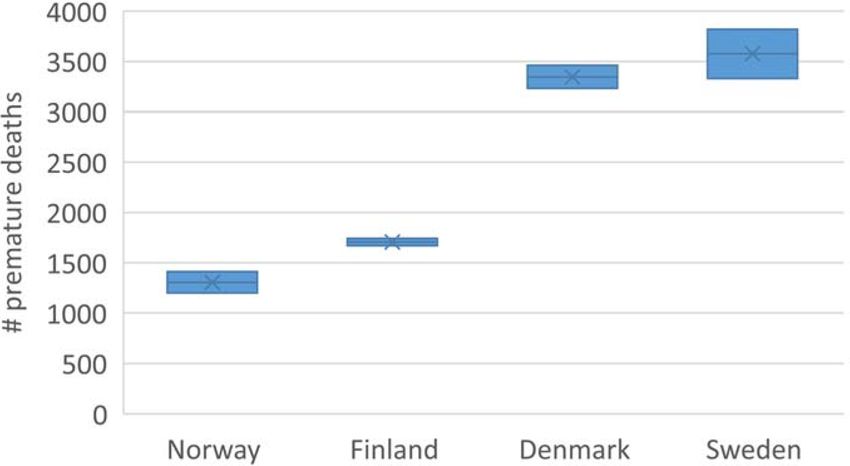
12504      C. Geels et al.: Projections of shipping emissions and the related impact on air pollution in the Nordic region

Table 2. Estimated emissions of CO2 , SO2 , NOx and BC for the polar diversion routes in domain d03 in 2020, 2030 and 2050.

                                               Diversion emission contribution        % emission increase due to diversion
                 Scenario              Year     CO2      SO2       NOx          BC     CO2        SO2      NOx        BC
                                                 Mt       Kt        Kt            t      %          %       %          %
                 BAU Baseline          2020     0.92     1.41      24.7         23         3        6         3          3
                                       2030     1.06     1.53      22.3         26         3        6         4          3
                                       2050     3.67     4.78      48.1         87         9       18        16          9
                 BAU SECA              2020     0.91     0.46      24.7         21         3         3        3          3
                                       2030     1.06     0.52      22.3         24         3         3        4          3
                                       2050     3.66     1.70      48.1         81         9         9       16          9
                 BAU HFO ban           2020     0.91     0.45      24.7         19         3         3        3          3
                                       2030     1.05     0.50      22.3         22         3         3        4          3
                                       2050     3.65     1.61      48.1         69         9         9       16          9
                 HiG HFO Baseline      2020     1.19     1.81    32.0            30        4        7         4         4
                                       2030     3.06     4.40    64.6            76        8       16        10         8
                                       2050    18.77    24.53   246.4           451       33       65        62        33

lowest for Norway (1300 ± 8 %) and Finland (1700 ± 2 %),                  but the MATCH-EVA numbers are for all countries lower
while it is highest for Sweden (3600 ± 7 %).                              than EEA and DEHM-EVA. This is in line with the under-
   For Denmark the total number of premature deaths is only               estimation the MATCH model shows for PM in the applied
slightly lower (3300 ± 3 %). Part of the difference between               setup.
the countries is of course related to difference in the popu-
lation numbers, where Sweden with a population of about
9.9 million (in 2015) is by far is the largest in the Nordic re-          3.3    Future developments in Nordic air pollution and
gion (see Table S4). The high number of premature deaths in                      health effects
Denmark, where the total population is only slightly higher
than in Norway, can be explained by the higher air pollu-
                                                                          The annual mean PM2.5 concentration as simulated by both
tion levels across Denmark (see Fig. 4a and b). In all coun-
                                                                          models for the BAU Baseline 2050 scenario is seen in Fig. 4c
tries the number of premature deaths attributable to long-
                                                                          and d. The land-based emissions of, e.g. NOx and SOx ,
term exposure to PM2.5 is a factor of 2–4 higher than the
                                                                          are projected to decrease in most of Europe in the applied
number of premature deaths attributable to acute effects. The
                                                                          ECLIPSE V5a scenarios (see Table S1). This leads to sig-
DEHM-EVA setup also covers Iceland and the Faroe Islands,
                                                                          nificant general reductions in the annual mean PM2.5 lev-
where the total number of premature deaths are estimated to
                                                                          els in most parts of the Nordic region towards 2050 (see
be approximately 40 and approximately 15, respectively, in
                                                                          Fig. 4e and f for the change in percentage). Parts of Rus-
2015. MATCH-EVA excludes these regions to the benefit of
                                                                          sia (e.g. around Murmansk and Saint Petersburg) and parts
a higher resolution in a smaller domain.
                                                                          of Norway stand out as exceptions, where the emissions, and
   The current assessment can be compared to the recent
                                                                          hence the PM2.5 concentration, are projected to increase. In
European Environment Agency (EEA) “Air quality in Eu-
                                                                          the MATCH results, the concentration in the Oslo region is
rope — 2018 report” (EEA, 2018), where premature deaths
                                                                          projected to increase by a few percent. This is not seen in
attributable to total PM2.5 , NO2 and O3 exposure are es-
                                                                          the DEHM results. Potential causes to this are the slightly
timated for 41 European countries for the year 2015. The
                                                                          lower resolution in the DEHM setup, differences in chemi-
EEA specifies that the uncertainty related to the health esti-
                                                                          cal scheme and differences in long-range-transported (LRT)
mates is ± 35 % (PM2.5 ), ± 45 % (NO2 ) and ± 50 % (O3 ). In
                                                                          component from continental Europe (the LRT component is
Fig. 6 the EEA estimates for PM2.5 mortality in four of the
                                                                          weaker in MATCH), possibly partly due to differences in me-
Nordic countries are compared to the current DEHM-EVA
                                                                          teorological forcing. Thus, although there is a general de-
and MATCH-EVA estimates based on the Baseline 2015 sim-
                                                                          crease in exposure to PM2.5 , some areas are projected to pos-
ulations, including both land-based and shipping emissions.
                                                                          sibly experience increased exposure.
Overall, the estimates are very similar for the four countries,
                                                                             For 2050 the difference between the BAU Baseline simu-
and some differences should be expected due to methodolog-
                                                                          lations and the simulations including the BAU SECA, BAU
ical differences. The DEHM-EVA and MATCH-EVA esti-
                                                                          HFO ban and HiG Baseline shipping scenarios (land-based
mates are both within the error interval of the EEA estimates,
                                                                          emissions are unchanged in all scenarios) can be analysed

Atmos. Chem. Phys., 21, 12495–12519, 2021                                                  https://doi.org/10.5194/acp-21-12495-2021
C. Geels et al.: Projections of shipping emissions and the related impact on air pollution in the Nordic region 12505 Figure 4. The annual mean surface PM2.5 concentration [µg m−3 ] for 2015, 2050 and the percentage change as simulated by the two models. in detail based on the percentage difference maps given in In the HFO ban scenario (7c and d) a slightly larger de- Fig. 7. crease is seen in most of the domain, and the PM2.5 lev- With the SECA scenario (Fig. 7a and b), a small de- els along shipping routes in the Baltic and around Denmark crease in the PM2.5 concentration is seen outside the cur- are up to 1.5 % lower than in the Baseline, and like in the rent Baltic Sea and North Sea SECA areas compared to the SECA scenario the largest decrease (ca. 2 %) is seen along BAU scenario. Along the Norwegian coast, the two models part of the Norwegian coast in the MATCH simulation. These project a decrease in PM2.5 concentration between 0.6 %– changes in the PM2.5 levels are, as described in Sect. 3.1.2, 1.5 %, whereas smaller changes are seen across the other linked to decreased SO2 emission in both the SECA and HFO countries. ban shipping scenario, which leads to a decrease in the for- https://doi.org/10.5194/acp-21-12495-2021 Atmos. Chem. Phys., 21, 12495–12519, 2021
12506      C. Geels et al.: Projections of shipping emissions and the related impact on air pollution in the Nordic region

                                                                       areas of predicted increases in PM2.5 than DEHM (7700 pre-
                                                                       mature deaths).

                                                                       3.4   The contributions from shipping

                                                                       The specific model simulations with shipping emissions re-
                                                                       duced by 30 %, can for each scenario be used to quantify the
                                                                       contributions from shipping to both the air pollution levels
                                                                       and the related health impacts. In terms of the annual PM2.5
                                                                       concentration, the contribution from shipping for all scenar-
Figure 5. Premature deaths attributable to NO2 , O3 , SO2 and PM2.5    ios (given as % of total PM2.5 in Fig. 8) is highest along
exposure in the four largest Nordic countries in the base case for     shipping routes and in coastal regions, giving a similar spa-
2015 (including all of the main anthropogenic emission sources).       tial pattern for both the DEHM and the MATCH models.
The results are given as box plots, where the “x” indicates the cen-   For the current 2015 Baseline, about 7 %–15 % of the annual
tral estimate and the size of the box shows the difference between     mean PM2.5 concentration over the majority of the Nordic
the DEHM-EVA and MATCH-EVA assessments.                                land area is linked to shipping in the DEHM results, while
                                                                       the MATCH results point to 1 %–10 % for the same areas.
                                                                       This is in line with a recent study based on the EMEP model,
                                                                       where the contribution from shipping to the averaged PM2.5
                                                                       concentration in the Nordic countries ranged from about 5 %
                                                                       in Finland to about 13 % in Denmark (Jonson et al., 2020).
                                                                          From Fig. 8c–g it can be seen that only small changes are
                                                                       projected for this contribution in the future according to the
                                                                       MATCH model, while the DEHM results for both the BAU
                                                                       2050 scenario and the HFO ban 2050 scenario show a de-
                                                                       crease in part of the area. The increased traffic in the HiG
                                                                       Baseline scenario increases the overall contribution from
                                                                       shipping, and thus it is higher than in 2015.
                                                                          The estimated number of premature deaths attributable to
                                                                       shipping can be seen in Fig. 9a. As a mean over the two
                                                                       models this amounts to approximately 850 premature deaths
Figure 6. Comparison between the assessment of premature deaths        under present-day conditions, decreasing to just below 600
reported by EEA for 2015 and the current assessment (base case         cases in the 2050 BAU Baseline scenario and to about 580
2015) for effects related to PM2.5 exposure. The EEA number in-        and 550 in the BAU SECA and BAU HFO ban scenarios.
cludes an error bar displaying the assumed uncertainty (± 35 %).       In the HiG Baseline scenario this number is projected to in-
                                                                       crease to almost 900 cases and hence to a value that is slightly
                                                                       higher than today. Details on numbers for each country are
mation of secondary inorganic aerosols and hence total PM              given in Fig. S6 in the Supplement. In Fig. 9b the result-
mass. The HFO ban scenario also includes a decrease in the             ing differences in the number of premature deaths in 2050
BC, which leads to small decrease in the primary PM part in            is shown. Only a small decrease (> −20 premature deaths)
the models.                                                            is seen for the SECA scenario. The HFO ban scenario has
   The HiG scenario will, on the other hand, result in an in-          a somewhat larger effect and would decrease the number of
crease in the PM2.5 concentration compared to the BAU sce-             premature deaths in 2050 with almost 50 cases in the Nordic
nario (Fig. 7e and f). Here an increase in the PM2.5 levels of         area compared to the BAU Baseline. The HiG scenario, on
up to 1 %–5 % is seen across Finland, Norway and Sweden                the other hand, is projected to increase the number of prema-
and is even higher over Denmark according to the DEHM                  ture deaths in the Nordic area by approximately 300 cases in
results. Somewhat lower values are seen in the MATCH re-               2050.
sults.                                                                    A recent study finds that long-term exposure to PM2.5
   In terms of health impacts resulting from the developments          from shipping can be associated with 5.5 premature deaths
in total BAU emissions the total number of 9900 ± 10 %                 per 100 000 inhabitants per year in eight Mediterranean
(mean of DEHM-EVA and MATCH-EVA) in 2015 is pro-                       coastal cities (Viana et al., 2020). For comparison, the 850
jected to decrease to about 8300 (only DEHM-EVA) in 2030               deaths in the Nordic area corresponds to approximately
and further to 7900 ± 6 % in 2050 in the current study. The            3.2 premature deaths per year per 100 000 inhabitants. This
MATCH-EVA setup gives the highest number of premature                  is somewhat lower than the number for the Mediterranean
deaths in 2050 (8200 premature deaths), mainly due to larger           cities, but this seems reasonable since several of the included

Atmos. Chem. Phys., 21, 12495–12519, 2021                                              https://doi.org/10.5194/acp-21-12495-2021
C. Geels et al.: Projections of shipping emissions and the related impact on air pollution in the Nordic region 12507 Figure 7. The percentage difference between the BAU Baseline 2050 simulation and the three different ship emission scenarios (in- cluding the polar diversion route) as simulated by the two models DEHM (a, c, e) and MATCH (b, d, f). Calculated as, e.g. (2050BAU_SECA − 2050BAU) / 2050BAU · 100 %. https://doi.org/10.5194/acp-21-12495-2021 Atmos. Chem. Phys., 21, 12495–12519, 2021
12508      C. Geels et al.: Projections of shipping emissions and the related impact on air pollution in the Nordic region

Figure 8. The contribution from shipping to the PM2.5 annual levels as simulated by the two models for the present day and three different
shipping emission scenarios for 2050. Calculated using, e.g. (2015BAU − 2015BAU_70 % / 0.3) / 2015BAU · 100 %, where 2015BAU_70 is
a run where the shipping emissions have been reduced to 70 %.)

Atmos. Chem. Phys., 21, 12495–12519, 2021                                                https://doi.org/10.5194/acp-21-12495-2021
C. Geels et al.: Projections of shipping emissions and the related impact on air pollution in the Nordic region 12509
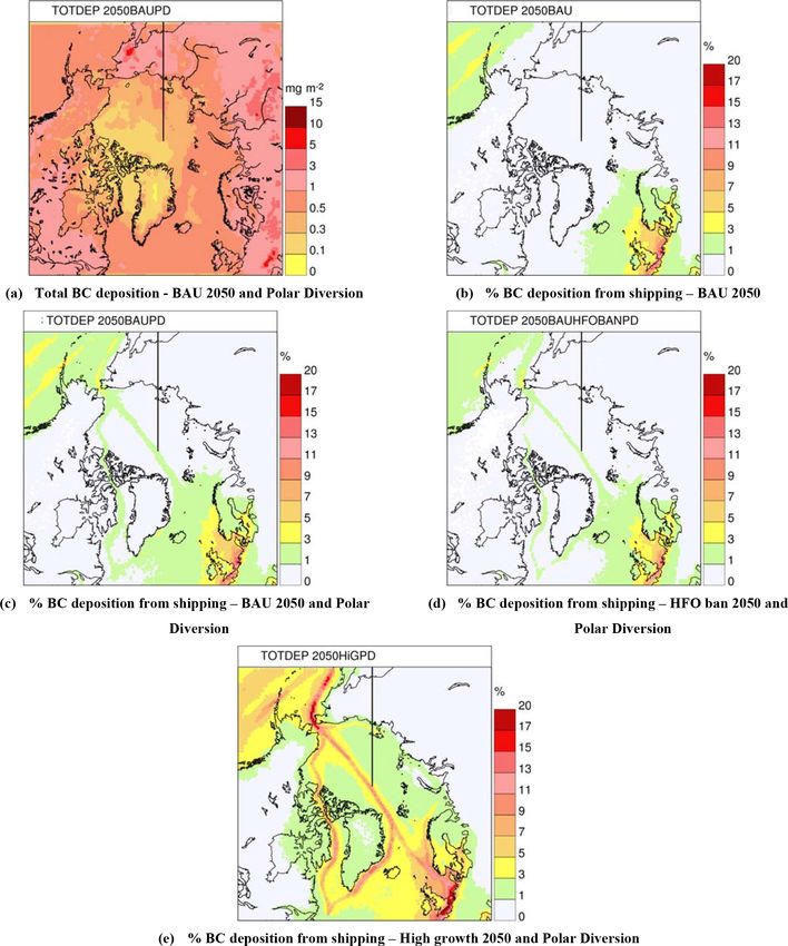
A map of the BC deposition is given in Fig. 10a for the
DEHM BAU Baseline 2050 simulation (for the d02 domain
with a horizontal resolution of 50 km × 50 km). The depo-
sition of BC under both present day and future conditions
show the same overall pattern, with a gradient towards the
Arctic area, where the deposition level is low (< 1 mg m−2 ).
With the included emissions in the Baseline scenario (includ-
ing both land-based and shipping emissions), the deposition
is projected to decrease by −1 % to −10 % across the Arc-
tic towards 2050. The overall contribution from shipping to
the BC deposition in the Arctic is very low and below 1 %
in most of the Arctic area, as can be seen from Fig. 10b (the
pattern is very similar for the 2015 simulation). In the simu-
lation including the new diversion shipping routes (Fig. 10c),
contributions of up to 3 % can be seen along the ship routes
across the Arctic Sea and in Baffin Bay, along the coast
of Ellesmere Island, Canada and Northwest Greenland. The
contribution will be higher during summer, when the ship-
ping activity along these routes peaks. In 2050 the emission
along the new diversion routes will constitute approximately
50 % of the BC related to shipping in the area.
Figure 9. (a) The estimated number of premature deaths attributable As described in Sect. 3.1 for the Nordic region, the future
to shipping. The difference between 2050BAU and 2050BAU_PD mitigation scenario with an HFO ban will have the largest
shows the impact from polar diversion routes. Note that the impact on the BC emissions, and for the Arctic this scenario
2030BAU and the SECA, HFO and HiG scenarios also includes leads to a decrease of about 12 % compared to the BAU Base-
the polar diversion routes. (b) Zoom in on the difference between
line for 2050 (see Winther et al., 2017 for details). When
the scenarios and BAU in 2050.
comparing the simulations, where the polar diversion route
is included, the results show that an HFO ban will lead to re-
cities in Spain and Italy are located in areas with significant ductions of a few percent in the BC deposition in the Arctic,
shipping activity. mainly along the shipping routes (Fig. 10d).
Like for PM2.5 described above, the contribution from In the scenario describing a high growth in the ship-
ships is around 11 % of the total number of premature deaths ping traffic (HiG), the contribution can increase to 5 %–15 %
when based on the DEHM-EVA simulation for 2015. When along the shipping routes as seen in Fig. 10e. Also in ar-
based on the parallel MATCH-EVA results, the estimated eas further away from the routes, a general increase in the
contribution from shipping is ca. 6 %. In the DEHM BAU contribution from shipping is seen. In an earlier study us-
Baseline, BAU SECA and BAU HFO ban simulations for ing a global model and a similar HiG scenario, Browse et al.
2030 this fraction increases somewhat to about 13 %, before (2013) found comparable increases in the contribution from
it decreases to ca. 9 % in the 2050 scenarios. In the HiG Base- shipping towards 2050 and they conclude that shipping could
line scenario the fraction is ca. 15 % in 2030, with a decrease have a significant impact on the albedo in this area. The de-
to 13 % in 2050. position of BC on snow and ice decreases the albedo and
The future scenarios discussed here all include the polar increases the absorption of incoming solar radiation, which
diversion as described in Sect. 3.1.3. To isolate the effect of can lead to earlier melting (AMAP, 2011).
this, simulations have been made with the 2050 BAU Base- Globally, observations and modelling results indicate that
line scenario with and without the polar diversion. In terms radiative forcing (RF) induced by BC on snow and ice is
of health effects, the additional emission leads to 10–30 pre- highest in the mid-latitudes (Bond et al., 2013; Kang et al.,
mature deaths in the Nordic area. 2020). While BC in the atmosphere can lead to a direct RF
of +0.71 W m2 , its semi- and indirect effects can be up to
3.5 Shipping and related depositions in the Arctic +0.23 W m2 . Sand et al. (2013) showed the Arctic (> 60◦ N)
sources of BC lead to a surface warming of 2.3 K, 1.6 K of
The second domain in the DEHM model (d02) covers the which is attributed to the effect from BC deposited on snow
Arctic region, and in the following the impact of the shipping and sea ice. Sand et al. (2016) estimated that BC in the at-
scenarios are briefly analysed for two components (BC and mosphere and snow leads to an Arctic warming of 0.48 K.
total nitrogen (N) deposition) within the Arctic area, where Sand et al. (2013, 2016) showed for per unit emissions that
we here focus on the modelled deposition of these compo- sources in the Arctic have a factor of 2 higher impact on Arc-
nents. tic warming compared to sources outside the Arctic. These
https://doi.org/10.5194/acp-21-12495-2021 Atmos. Chem. Phys., 21, 12495–12519, 2021You can also read