Impacts of household sources on air pollution at village and regional scales in India
←
→
Page content transcription
If your browser does not render page correctly, please read the page content below
Atmos. Chem. Phys., 19, 7719–7742, 2019
https://doi.org/10.5194/acp-19-7719-2019
© Author(s) 2019. This work is distributed under
the Creative Commons Attribution 4.0 License.

Impacts of household sources on air pollution at village and
regional scales in India
Brigitte Rooney1 , Ran Zhao2,a , Yuan Wang1,3 , Kelvin H. Bates2,b , Ajay Pillarisetti4 , Sumit Sharma5 , Seema Kundu5 ,
Tami C. Bond6 , Nicholas L. Lam6,c , Bora Ozaltun6 , Li Xu6 , Varun Goel7 , Lauren T. Fleming8 , Robert Weltman8 ,
Simone Meinardi8 , Donald R. Blake8 , Sergey A. Nizkorodov8 , Rufus D. Edwards9 , Ankit Yadav10 ,
Narendra K. Arora10 , Kirk R. Smith4 , and John H. Seinfeld2
1 Division of Geological and Planetary Sciences, California Institute of Technology, Pasadena, CA 91125, USA
2 Division of Chemistry and Chemical Engineering, California Institute of Technology, Pasadena, CA 91125, USA
3 Jet Propulsion Laboratory, California Institute of Technology, Pasadena, CA 91125, USA
4 School of Public Health, University of California, Berkeley, CA 94720, USA
5 The Energy and Resources Institute (TERI), New Delhi 110003, India
6 Department of Civil and Environmental Engineering, University of Illinois, Urbana-Champaign, IL 61801, USA
7 Department of Geography, University of North Carolina, Chapel Hill, NC 27516, USA
8 Department of Chemistry, University of California, Irvine, CA 92697, USA
9 Department of Epidemiology, University of California, Irvine, CA 92697, USA
10 The INCLEN Trust, Okhla Industrial Area, Phase-I, New Delhi 110020, India
a current address: Department of Chemistry, University of Alberta, Edmonton, Alberta, T6G 2R3, Canada
b current address: Center for the Environment, Harvard University, Cambridge, MA 02138, USA
c current address: Schatz Energy Research Center, Humboldt State University, Arcata, CA 95521, USA

Correspondence: John H. Seinfeld (seinfeld@caltech.edu) and Kirk R. Smith (krksmith@berkeley.edu)

Received: 14 November 2018 – Discussion started: 6 December 2018
Revised: 25 April 2019 – Accepted: 14 May 2019 – Published: 11 June 2019

Abstract. Approximately 3 billion people worldwide cook          of New Delhi. The DDESS covers an approximate popu-
with solid fuels, such as wood, charcoal, and agricultural       lation of 200 000 within 52 villages. The emissions inven-
residues. These fuels, also used for residential heating, are    tory used in the present study was prepared based on a na-
often combusted in inefficient devices, producing carbona-       tional inventory in India (Sharma et al., 2015, 2016), an up-
ceous emissions. Between 2.6 and 3.8 million premature           dated residential sector inventory prepared at the Univer-
deaths occur as a result of exposure to fine particulate mat-    sity of Illinois, updated cookstove emissions factors from
ter from the resulting household air pollution (Health Effects   Fleming et al. (2018b), and PM2.5 speciation from cooking
Institute, 2018a; World Health Organization, 2018). House-       fires from Jayarathne et al. (2018). Simulation of regional
hold air pollution also contributes to ambient air pollution;    air quality was carried out using the US Environmental Pro-
the magnitude of this contribution is uncertain. Here, we        tection Agency Community Multiscale Air Quality model-
simulate the distribution of the two major health-damaging       ing system (CMAQ) in conjunction with the Weather Re-
outdoor air pollutants (PM2.5 and O3 ) using state-of-the-       search and Forecasting modeling system (WRF) to simu-
science emissions databases and atmospheric chemical trans-      late the meteorological inputs for CMAQ, and the global
port models to estimate the impact of household combustion       chemical transport model GEOS-Chem to generate concen-
on ambient air quality in India. The present study focuses       trations on the boundary of the computational domain. Com-
on New Delhi and the SOMAARTH Demographic, Devel-                parisons between observed and simulated O3 and PM2.5 lev-
opment, and Environmental Surveillance Site (DDESS) in           els are carried out to assess overall airborne levels and to
the Palwal District of Haryana, located about 80 km south        estimate the contribution of household cooking emissions.

Published by Copernicus Publications on behalf of the European Geosciences Union.
7720 B. Rooney et al.: Household sources of air pollution in India
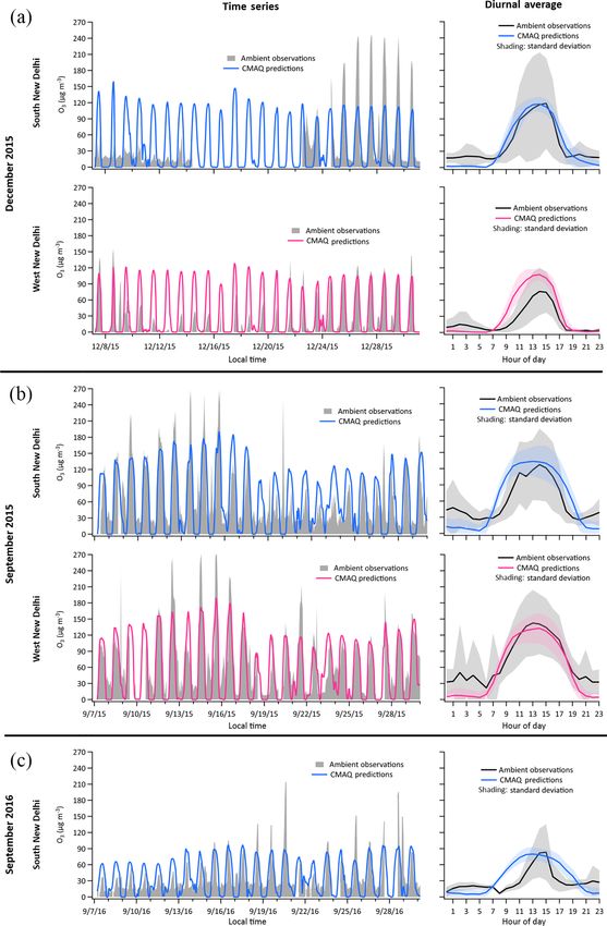
Observed and predicted ozone levels over New Delhi dur- ticulate matter from household air pollution (Health Effects
ing September 2015, December 2015, and September 2016 Institute, 2018a; World Health Organization, 2018). In In-
routinely exceeded the 8 h Indian standard of 100 µg m−3 , dia, more than 50 % of households report the use of wood or
and, on occasion, exceeded 180 µg m−3 . PM2.5 levels are pre- crop residues, and 8 % report the use of dung as cooking fuel
dicted over the SOMAARTH headquarters (September 2015 (Klimont et al., 2009; Census of India, 2011; Pant and Harri-
and September 2016), Bajada Pahari (a village in the surveil- son, 2012). Residential biomass burning is one of the largest
lance site; September 2015, December 2015, and Septem- individual contributors to the burden of disease in India, es-
ber 2016), and New Delhi (September 2015, December 2015, timated to be responsible for 780 000 premature deaths in
and September 2016). The predicted fractional impact of res- 2016 (Indian Council of Medical Research et al., 2017). The
idential emissions on anthropogenic PM2.5 levels varies from recent GBD MAPS Working Group (Health Effects Institute,
about 0.27 in SOMAARTH HQ and Bajada Pahari to about 2018b) estimated that household emissions in India produce
0.10 in New Delhi. The predicted secondary organic portion about 24 % of ambient air pollution exposure. Coal combus-
of PM2.5 produced by household emissions ranges from 16 % tion, roughly evenly divided between industrial sources and
to 80 %. Predicted levels of secondary organic PM2.5 dur- thermal power plants, was estimated by this study to be re-
ing the periods studied at the four locations averaged about sponsible for 15.3 % of exposure in 2015. Open burning of
30 µg m−3 , representing approximately 30 % and 20 % of to- agricultural crop stubble was estimated annually to be re-
tal PM2.5 levels in the rural and urban stations, respectively. sponsible for 6.1 % nationally, although it was higher in some
areas.
Traditional biomass cookstoves, with characteristic low
combustion efficiencies, produce significant gas- and
1 Introduction particle-phase emissions. An early study of household air
pollution in India found outdoor total suspended particu-
Although outdoor air pollution is widely recognized as a late matter (TSP) levels in four Gujarati villages well over
health risk, quantitative understanding remains uncertain on 2 mg m−3 during cooking periods (Smith et al., 1983). Sec-
the degree to which household combustion contributes to ondary organic aerosol (SOA), produced by gas-phase con-
unhealthy air. Recent studies in China, for example, show version of volatile organic compounds to the particulate
that 50 %–70 % of black carbon (BC) emissions and 60 %– phase, is also important in ambient PM levels, yet there is a
90 % of organic carbon (OC) emissions can be attributed dearth of model predictions to which data can be compared.
to residential coal and biomass burning (Cao et al., 2006; Overall, household cooking in India has been estimated by
Klimont et al., 2009; Lai et al., 2011). Moreover, existing various groups to produce 22 %–50 % of ambient PM2.5 ex-
global emissions inventories show a significant contribution posure (Butt et al., 2016; Chafe et al., 2014; Conibear et al.,
of household sources to primary PM2.5 (particulate matter of 2018; Health Effects Institute, 2018b; Lelieveld et al., 2015;
diameter less than or equal to 2.5 µm) emissions. The Indo- Silva et al., 2016), and Fleming et al. (2018a, b) report char-
Gangetic Plain of northern India (23–31◦ N, 68–90◦ E) has acterization of a wide range of particle-phase compounds
among the world’s highest values of PM2.5 . In this region, the emitted by cookstoves. In a multi-model evaluation, Pan et
major sources of emissions of primary PM2.5 and of precur- al. (2015) concluded that an underestimation of biomass
sors to secondary PM2.5 are coal-fired power plants, indus- combustion emissions, especially in winter, was the dom-
tries, agricultural biomass burning, transportation, and com- inant source of model underestimation. Here, we address
bustion of biomass fuels for heating and cooking (Reddy and both primary and secondary organic particulate matter from
Venkataraman, 2002; Rehman et al., 2011). The southwest household burning of biomass for cooking.
monsoon in summer months in India leads to lower pollution Air quality in urban areas in India is determined largely,
levels than in winter months, which are characterized by low but not entirely, by anthropogenic fuel combustion. In rural
wind speeds, shallow boundary layer depths, and high rela- areas, residential combustion of biomass for household uses,
tive humidity (Sen et al., 2017). With the difficulty in deter- such as cooking, also contributes to nonmethane volatile or-
mining representative emissions estimates (Jena et al., 2015; ganic carbon (NMVOC) and particulate emissions (Sharma
Zhong et al., 2016), simulating the extremely high PM2.5 ob- et al., 2015, 2018). Average daily PM2.5 levels frequently
servations in the Indo-Gangetic Plain has remained a chal- exceed the 24 h Indian standard of 60 µg m−3 and can ex-
lenge (Schnell et al., 2018). ceed 150 µg m−3 , even in rural areas. The local region on
Approximately 3 billion people worldwide cook with solid which the present study focuses is the SOMAARTH De-
fuels, such as wood, charcoal, and agricultural residues (Bon- mographic, Development, and Environmental Surveillance
jour et al., 2013; Chafe et al., 2014; Smith et al., 2014; Ed- Site (DDESS) run by the International Clinical Epidemiolog-
wards et al., 2017). Used also for residential heating, such ical Network (INCLEN) in the Palwal District of Haryana
solid fuels are often combusted in inefficient devices, pro- (Fig. 1). Located about 80 km south of New Delhi, SO-
ducing BC and OC emissions. Between 2.6 and 3.8 million MAARTH covers an approximate population of 200 000 in
premature deaths occur as a result of exposure to fine par- 52 villages. Particular focus in the present study is given
Atmos. Chem. Phys., 19, 7719–7742, 2019 www.atmos-chem-phys.net/19/7719/2019/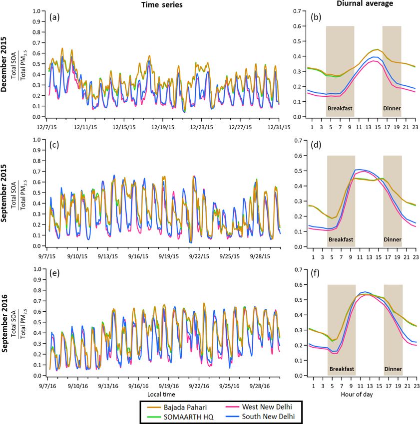
B. Rooney et al.: Household sources of air pollution in India                                                                7721

to the SOMAARTH Headquarters (HQ) and the village of              equation:
Bajada Pahari within DDESS, coinciding with the work of                 XXX
Fleming et al. (2018b), who studied cookstove nonmethane          Ek =      Ak,l,m efk,l,m 1 − ηl,m,n · Xk,l,m,n ,             (1)
                                                                         l   m   n
hydrocarbon (NMHC) emissions and ambient air quality.
Demographically, with a coverage of almost 308 km2 , the          where E denotes the pollutant emissions (in kt); k, l, m,
DDESS has a mix of populations from different religions and       and n are region, sector, fuel or activity type, and control
socioeconomic and development statuses.                           technology, respectively; A is the activity rate; ef is the un-
   The climate of the region of interest in the present study     abated emission factor (kt per unit of activity); η is the re-
is primarily influenced by monsoons, with a dry winter and        moval efficiency (%/100); and X is the   P application rate of
very wet summer. The rainy season, July through Septem-           control technology n (%/100) where X = 1. The energy
ber, is characterized by average temperatures around 30 ◦ C       sources considered include coal, natural gas, petroleum prod-
and primarily easterly and southeasterly winds. In a study        ucts, biomass fuels, and others and are categorized into five
related to the present one, Schnell et al. (2018) used emis-      sectors – transport, industries, residential, power, and oth-
sion datasets developed for the Coupled Model Intercompar-        ers. The model uses the state-wise energy data and gener-
ison Project Phases 5 (CMIP5) and 6 (CMIP6) to evaluate           ates emissions of species such as PM, NOx , SO2 , NMVOCs,
the impact on predicted PM2.5 over northern India, October–       NH3 , and CO.
March 2015–2016, with special attention paid to the effect           For activity data of source sectors, TERI employed pub-
of meteorology of the region, including relative humidity,        lished statistics (mainly population, vehicle registration, en-
boundary layer depth, strength of the temperature inversion,      ergy use, and industrial production) where possible. Energy-
and low-level wind speed. In that work, nitrate and organic       use data for industry and power sectors were compiled based
matter (OM) were predicted to be the dominant components          on a bottom-up approach, collected from the Ministry of
of total PM2.5 over most of northern India.                       Petroleum and Natural Gas (MoPNG, 2010), the Central
   The goal of the present work is to simulate the distribution   Statistics Office (CSO, 2011), and the Central Electricity Au-
of primary and secondary PM2.5 and O3 using recently up-          thority (CEA, 2011). Transportation activity data were com-
dated emissions databases and atmospheric chemical trans-         piled from information on vehicle registrations (Ministry of
port models to obtain estimates of the total impact on am-        Road Transport and Highways, 2011), emission standards
bient air quality attributable to household combustion. With      (MoPNG, 2001), travel demand (CPCB, 2000), and mileage
respect to ozone, the present work follows that of Sharma         (TERI, 2002). Emission factors for energy-based sources
et al. (2016), who simulated regional and urban ozone con-        from the GAINS ASIA database were used. Speciation fac-
centrations in India using a chemical transport model and in-     tors are adopted from sector-specific profiles from Wei et
cluded a sensitivity analysis to highlight the effect of chang-   al. (2014), primarily developed for China as there is a lack
ing precursor species on O3 levels. The present work is based     of information for India. In the transportation sector, the Chi-
on simulating the levels of both O3 and PM2.5 at the regional     nese species profiles are dependent on fuel type but not tech-
level based on recent emissions inventories using state-of-       nology.
the-science atmospheric chemical transport models.                   The TERI inventory was compiled on a yearly basis, with
                                                                  monthly variations for brick kilns and agricultural burning, at
                                                                  a native resolution of 36 km × 36 km then equally distributed
2     Emissions inventory                                         to grid resolution of 4 km × 4 km for this study. Emissions
                                                                  for nonresidential sectors have no specified diurnal or daily
2.1    Nonresidential sectors emissions                           variations; thus, the inventory for nonresidential sectors is the
                                                                  same for each simulated day. Transportation sector emissions
The present study uses an emissions inventory conglomer-          were estimated using population and vehicle fleet data at the
ated from two primary sources: (1) an India-scale inventory       district level and distributed to the grid using the adminis-
for all nonresidential sectors prepared by TERI (Sharma et        trative boundaries. Industry, power, and oil and gas sector
al., 2015, 2016) and (2) a high-resolution residential sector     emissions were assigned to the grid by their respective lo-
inventory detailed here. Emissions data from each source          cations. Emissions from agriculture were allocated by crop-
were distributed to a 4 km grid for the present study. The        types produced by state in India. The inventory was vertically
TERI national inventory was prepared at a resolution of           distributed to three layers with the lowest layer extending to
36 km × 36 km using the Greenhouse Gas and Air Pollu-             30–43 m, the middle layer to 75–100 m, and the top layer
tion Interactions and Synergies (GAINS ASIA) emission             to 170–225 m. Volatile organic compound (VOC) emissions
model (Amann et al., 2011). GAINS ASIA estimated emis-            were assumed to occur only in the bottom layer. Industry and
sions based on energy and nonenergy sources using an emis-        power emissions were distributed based on stack heights and
sion factor approach after taking into account various fuel-      allocated to the second and third layers.
sector combinations. Following the approach of Kilmont et            We incorporated biogenic emissions by using daily-
al. (2002), the emissions were estimated using the basic          averaged emission rates of isoprene (0.8121 moles s−1 ) and

www.atmos-chem-phys.net/19/7719/2019/                                                Atmos. Chem. Phys., 19, 7719–7742, 2019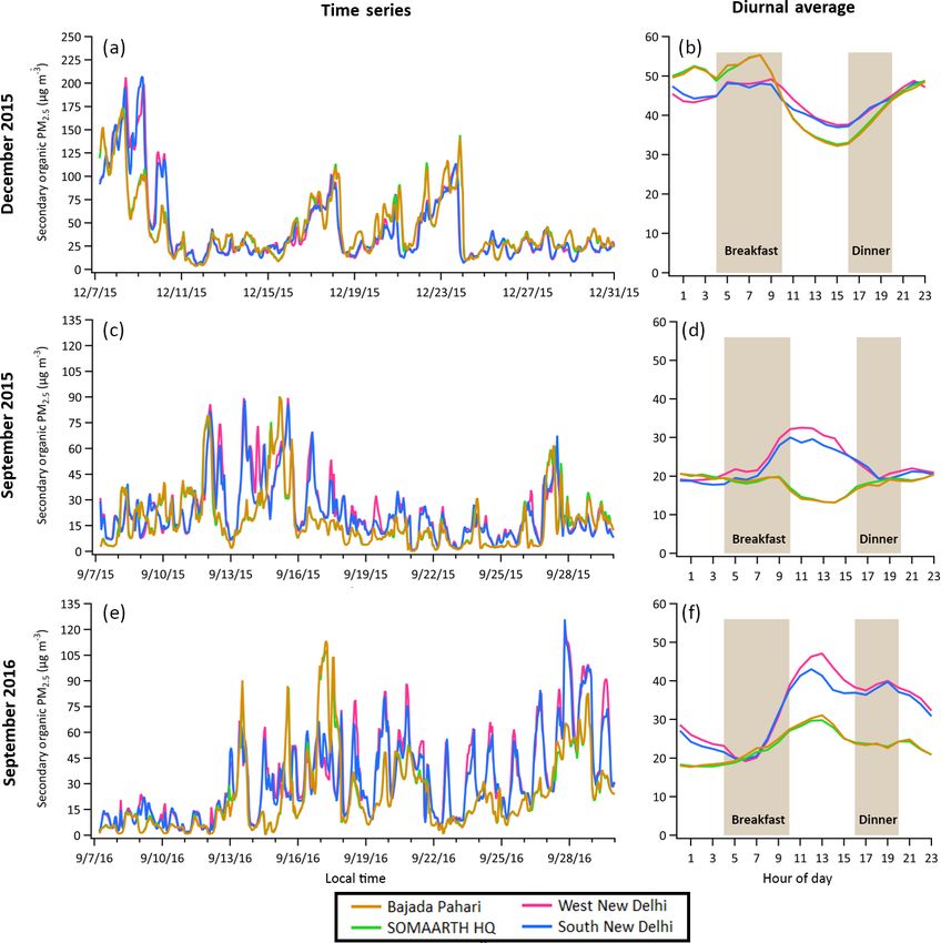
7722 B. Rooney et al.: Household sources of air pollution in India
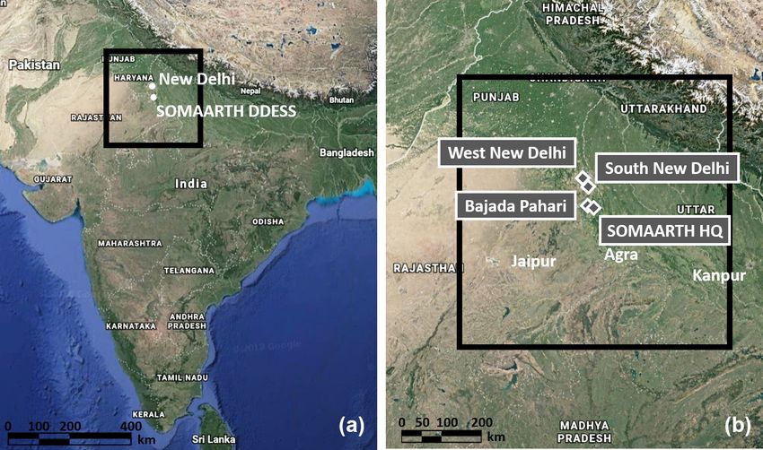
Figure 1. Geographic area of simulation. Panel (a) shows the entirety of India, and (b) shows a close-up of the model domain. The domain
spans a 600 km by 600 km area with a grid resolution of 4 km (150 cells along each axis) and includes both New Delhi and SOMAARTH
DDESS.
terpenes (0.8067 moles s−1 ) per 4 km grid cell, predicted by Hourly emissions were generated using source-specific diur-
GEOS-Chem for the region of study. The TERI inventory nal emissions profiles (Fig. 2). The same diurnal emissions
additionally includes isoprene emissions from the residential profile is applied to all species from a source category and
sector, so isoprene from natural sources was calculated as the was informed by real-time emissions measurements taken in
difference of the total rate predicted by GEOS-Chem and the homes during cooking reported by Fleming et al. (2018a, b).
rate of emissions solely from the residential sector. Terpene Profiles for fuel-based lighting were informed by real-time
emissions are assumed to occur only in nonresidential source measurements of kerosene lamp usage data reported in Lam
sectors. Isoprene and terpene emission rates were applied to et al. (2018). The residential sector inventory represents sur-
all computational cells as an hourly average (with no diurnal face emissions with a native spatial resolution of 30 arcsec
profile) in the nonresidential inventory. (∼ 1 km).
In deriving summary estimates of emission factors, prior-
2.2 Residential sector emissions ity was given to emission factor measurements from field-
based studies. Several studies have shown that laboratory-
To examine local and regional impacts of residential sec- based measurements of stove and lighting emissions tend to
tor emissions in greater detail, an update to the TERI in- be lower than those of devices measured in actual homes
ventory was performed using various sources to consider (Roden et al., 2009), perhaps due to higher variation in fuel
more granular input data specific to the residential sector quality and operator behavior. Field-based emission factors
(Table 1). Bottom-up estimates of delivered energy for cook- utilized in this study include those for nonmethane hydro-
ing, space heating, water heating, and lighting were informed carbons, measured from fuels and stoves within the study
by those used in Pandey et al. (2014) and converted to fuel domain (Fleming et al., 2018a, b). PM2.5 speciation from
consumption at the village level using population size and cooking fires was informed by Jayarathne et al. (2018) (Ta-
percentage of reported primary cooking and lighting fuels bles 2 and 3). Residential emission rates for PM2.5 , BC, OC,
from the 2011 Census of India (2011). Urban areas of the CO, NOx , CH4 , CO2 , and NMHCs were generated from
domain were assumed to have the average cooking and light- SPEW, which estimates emissions from combustion by fuel
ing fuel use profiles of the average urban areas of their dis- type. As such, solvent emissions are not included for lack
trict. Fuel consumption was converted to emission rates using of specific input data. Additionally, while SPEW incorpo-
fuel-specific emission factors informed by a review of field rates temperature-dependent heating combustion activity, the
and laboratory studies, which was used to update the Speci- inventory assumes temperatures too high for this activity to
ated Pollutant Emissions Wizard (SPEW) inventory (Bond et
al., 2004) and to generate summary estimates by fuel type.
Atmos. Chem. Phys., 19, 7719–7742, 2019 www.atmos-chem-phys.net/19/7719/2019/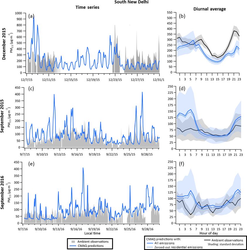
B. Rooney et al.: Household sources of air pollution in India                                                                                                      7723

Table 1. Residential emissions inventory sources by species.

                   CMAQ required           Source                                                                                              Solely emitted by
                   species1                                                                                                                    residential sector
                   NO                      Tami C. Bond (University of Illinois) NOx using Sharma et al. (2015),                               No
                                           NO : NO2 = 10 : 1
                   NO2                                                                                                                         No
  Gas              SO2                     Sharma et al. (2015)                                                                                No
                   NH3                     Sharma et al. (2015), assumed to be negligible
                   CO                      Tami C. Bond (University of Illinois)                                                               No
                   ALD2                                                                                                                        No
                   ALDX                                                                                                                        Yes
                   ETH                                                                                                                         No
                   ETHA                                                                                                                        No
  NMHC             ETOH                    Speciation from Tami C. Bond (University of Illinois) NMHC                                          No
                   FORM                    using Fleming et al. (2018a, b) emission factors                                                    No
                   MEOH                                                                                                                        No
                   OLE                                                                                                                         No
                   PAR3calculated                                                                                                              No
                   TOL                                                                                                                         No
                   XYL3                                                                                                                        No
                   ISOP2                   All-sector total ISOP emission from GEOS-Chem daily average and subtracted                          No
                                           nonresidential ISOP emission from Sharma et al. (2015)
  CMAQ             TERP2                   Assumed to be negligible
  AERO6            XYLMN                   XYLMN = 0.998 × XYL                                                                                 No
  species          NAPH                    NAPH = 0.002 × XYL                                       Pye and Pouliot (2012)                     No
                   PARCMAQ                 PARCMAQ =                                                                                           No
                                           PARcalculated − 0.00001 × NAPH
                   SOAALK                  SOAALK = 0.108 × PARCMAQ                                                                            No
                   PEC                     Tami C. Bond (University of Illinois)                                                               No
                   POC                                                                                                                         No
                   PNA                                                                                                                         Yes
                   PCL                                                                                                                         Yes
                   PK                      Speciation of PM2.5 from Tami C. Bond (University of Illinois) using                                Yes
                   PNH4                    Jayarathne et al. (2018) mass percentage                                                            Yes
                   PNO3                                                                                                                        No
                   PSO4                                                                                                                        No
  PM               PMOTHR                  PMOTHR = PM2.5 − (PEC + POC + PNA + PNH4 + PK + PCL + PNO3 + PSO4 )                                 No
                   PMC                     Sharma et al. (2015)                                                                                No
                   PNCOM                   Unknown, assumed to be 0
                   PH2 O
                   PAL
                   PCA
                   PFE                     Assumed to be negligible
                   PMG
                   PMN
                   PSI
                   PTI
1 Bolded species contribute to SOA production via the AERO6 module. 2 Total isoprene and terpene emissions from all sectors are taken from GEOS-Chem and were included
only in the O3 simulations. 3 PARcalculated and XYL are excluded from CMAQ and replaced with PARCMAQ , XYLMN, NAPH, and SOAALK.

www.atmos-chem-phys.net/19/7719/2019/                                                                         Atmos. Chem. Phys., 19, 7719–7742, 2019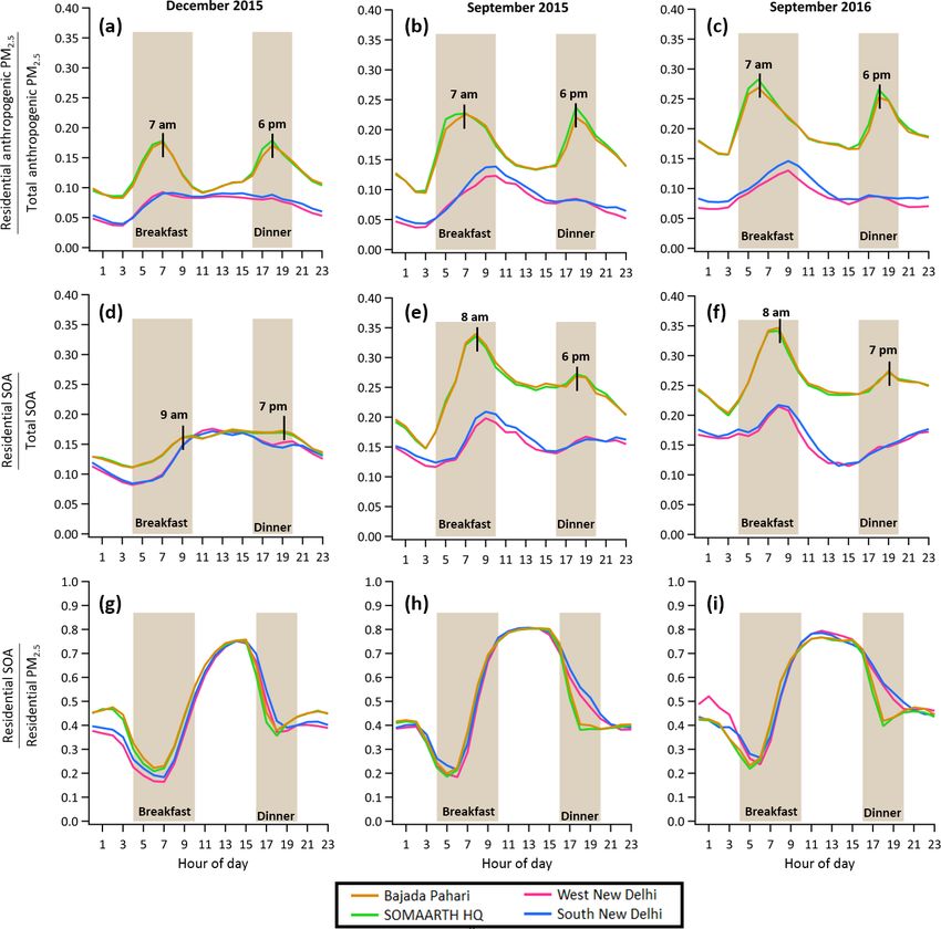
7724                                                                      B. Rooney et al.: Household sources of air pollution in India

Figure 2. Fraction of daily household emissions by quantifiable
fuel-use activity. Red, green, blue, and purple indicate cooking,
space heating, water heating, and lighting, respectively. This rep-          Figure 3. Fuel type assumed for speciation of household NMHC
resents the fraction of activity-specific daily emissions at each hour.      emissions. Study domain: 600 km by 600 km at 4 km resolution.
Each species obeys the same profile. While profiles for heating are          Red indicates cells where dung use dominated emissions and thus
shown, the inventory assumes temperatures too high for this activity         was assumed to be the sole fuel type used. Orange indicates cells
to take effect.                                                              where wood and agricultural residue use dominated emissions and
                                                                             was thus assumed to be the sole fuel type used.

take effect. Thus, our inventory has no emissions from heat-
                                                                             assumed to be negligible owing to a lack of information on
ing.
                                                                             these species. Emissions of remaining particle-phase species
   We employed various methods to account for pollutant
                                                                             (i.e., Al, Ca, Fe, Mg, Mn, Si, and Ti) were also assumed to
species not explicitly reported by SPEW (Tables 1 and 2).
                                                                             be negligible for lack of information. Unspeciated fine par-
Gas-phase SO2 and NH3 emissions were informed by exist-
                                                                             ticulate matter (PMothr ) is defined in CMAQ as the portion of
ing residential emissions in the TERI inventory (Sharma et
                                                                             total PM2.5 unassigned to any other species:
al., 2015); NO and NO2 were estimated from NOx emissions,
assuming a NO : NO2 emission ratio of 10 : 1. Total NMHC
                                                                             PMothr = PM2.5 − PEC + POC + PNa + PNH4 + PK                 (2)
and PM2.5 emission factors from SPEW are distributed by
fuel type (wood, dung, agriculture residue, or LPG) (Table 2).                        +PCl + PNO3 + PSO4
Given the low PM2.5 emission rate of LPG (Shen et al.,
                                                                             Tables 4 and 5 summarize emission rates for the study do-
2018), emissions from LPG are assumed to be negligible. To
                                                                             main.
further speciate NMHCs, we employed HC species-specific
emission factors (Fleming et al., 2018b), differentiated by
fuel and stove type (i.e., traditional stove, or chulha, with                3   Atmospheric modeling
wood or dung, and simmering stove, or angithi, with dung).
We assume that all NMHC emissions in each computational                      To study the impact of household emissions on ambient
grid cell are produced by either wood or dung, whichever                     air pollution, we simulated two emission scenarios each for
contributes the greater fraction of total PM2.5 emissions in                 three time periods which coincide with available INCLEN
that cell (Fig. 3). The NMHC emission profile of dung was                    observation data (Tables 6 and 7). A “total” emission sce-
assumed to be the average of measurements from chulha and                    nario represents the overall atmospheric environment by in-
angithi stoves. The emission profile for agricultural residue                cluding emissions from all source sectors in the inventory.
is similar to that of wood; therefore, wood speciation profiles              A “nonresidential” emission scenario represents zeroing-out
are applied in cells where agricultural residue dominates.                   or “turning-off” of all household emissions. By considering
   Particle-phase speciation of total PM2.5 was based on PM                  these scenarios independently, we can isolate the effect of
mass emissions from wood- and wood–dung-fueled cook-                         the residential sector on the ambient atmosphere. Each sce-
ing fires as reported by Jayarathne et al. (2018), and pri-                  nario was simulated over a region in northern India (Fig. 1)
mary cooking fuel type distribution data from the 2011 cen-                  for those periods when measurements were carried out in
sus (Tables 2 and 3). A single PM2.5 speciation profile, de-                 the region of interest. Figure 1 shows the 600 km by 600 km
fined as the average of that of wood and that of the wood–                   domain with 4 km grid resolution. The domain is centered
dung mixture, was applied in all cells for lack of information               over the Palwal District and the SOMAARTH DDESS and
on pure dung emissions (Table 3). Noncarbon organic par-                     includes New Delhi and portions of surrounding states.
ticulate matter (PNCOM ) and particulate water (PH2 O ) were

Atmos. Chem. Phys., 19, 7719–7742, 2019                                                       www.atmos-chem-phys.net/19/7719/2019/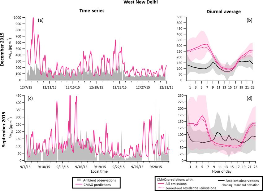
B. Rooney et al.: Household sources of air pollution in India                                                                                                  7725

Table 2. Residential PM2.5 and NMHC emissions speciation.

               Emitted species                           Fuel-specific                  Use
                                                         data
               PM2.5                                     Wood, dung,                    Total PM2.5 emission rate distributed by wood, dung, and agri-
               (Bond et al., 2004)                       agricultural                   cultural residue.
                                                         residue, LPG                   LPG emissions assumed to be negligible.
               Speciated PM2.5                           Wood,    wood–                 Average profile of wood and wood–
               (Jayarathne et al., 2018)                 dung mix                       dung mix applied to all fuel type emissions.
               NMHC                                      Wood, dung,                    Total PM2.5 emission rate distributed by wood, dung, and agri-
               (Bond et al., 2004)                       agricultural                   cultural residue.
                                                         residue, LPG                   LPG emissions assumed negligible.
               Speciated HCs                             Wood, dung                     One profile applied to each cell according to which fuel type
               (Fleming et al., 2018a, b)                                               dominates emissions in that cell.
                                                                                        Where agricultural residue dominates, wood profile is assumed.

Table 3. PM2.5 speciation by fuel type.                                                         Table 4. Particulate matter surface emissions over study domain.

                                    % mass of total emitted PM2.5                                                                                  % emitted by
    Emitted species1                                                                                                                                 residential
                                                                      Average
                               Wood2         Wood–dung2                                               Species                   Emission rate             sector
                                                                    employed3
                                                                                                                    POC                1.48 ×10⁶          30.78
    PEC                             14                   5.10               9.55
                                                                                                                    PEC                7.18 ×10⁵          15.89
    POC                             52                     61              56.50
    PNA                           0.05                   0.39               0.22                                    PCL                1.69 ×10³            100
    PCL                           3.20                   8.58               5.89                      Particulate   PK                 4.61 ×10³            100
    PK                            1.78                   0.52               1.15                      matter        PNA                2.46 ×10⁴          10.07
    PNH4                          1.12                   4.46               2.79                      (kg d−1 )     PNH4               2.11 ×10⁵           1.47
    PNO3                          0.42                   0.21               0.32                                    PNO3               6.51 ×10⁵          27.90
    PSO4                          0.33                   0.46               0.40                                    PSO4               1.18 ×10⁶          61.45
    PMOTHR                       27.10                  19.29              23.19                                    PMC                9.00 ×10³            100
  1 Total PM
                                                                                                                    PMOTHR             2.18 ×10⁴            100
             2.5 mass emission rates from residential combustion were estimated
  and distributed by fuel type (wood, dung, or agricultural residue) by University                    SOA           NAPH               6.82 ×10³           2.72
  of Illinois. 2 Emitted PM2.5 weight percent reported by Jayarathne et
  al. (2018). 3 An average profile applied to all cells, indiscriminate of fuel type.                 precursor     SOAALK             3.75 ×10⁶          34.54
                                                                                                      VOCs          TOL                1.54 ×10⁶          27.21
                                                                                                      (mol d−1 )    XYLMN              3.40 ×10⁶           2.72
   Simulation of regional air quality was carried out using
the US Environmental Protection Agency Community Mul-
tiscale Air Quality modeling system (CMAQ), version 5.2                                         cal transport model GEOS-Chem v11-02c (http://acmg.seas.
(Appel et al., 2017; US EPA, 2017). CMAQ is a three-                                            harvard.edu/geos/index.html, last access: 28 May 2019) to
dimensional chemical transport model (CTM) that predicts                                        generate concentrations on the boundary of the computa-
the dynamic concentrations of airborne species. CMAQ in-                                        tional domain. Meteorological conditions (including temper-
cludes modules of radiative processes, aerosol microphysics,                                    ature, relative humidity, wind speed and direction and land
cloud processes, wet and dry deposition, and atmospheric                                        use and terrain data) drive the atmospheric processes rep-
transport. Required input to the model includes emissions in-                                   resented in CMAQ. The Weather Research and Forecasting
ventories, initial and boundary conditions, and meteorologi-                                    modeling system (WRF) Advanced Research WRF (WRF-
cal fields. The domain-specific, gridded emissions inventory                                    ARW, version 3.6.1) was used to simulate the meteorological
provides hourly-resolved total emission rates for each species                                  input for CMAQ (Skamarock et al., 2008).
(not differentiated by source) by cell, time step, and vertical
layer. Initial conditions (ICs) and boundary conditions (BCs)                                   3.1    GEOS-Chem
are necessary to define the atmospheric chemical concentra-
tions in the domain at the first time step and at the domain                                    We used GEOS-Chem v11-02c, a global chemical trans-
edges, respectively. The present study uses the global chemi-                                   port model driven by assimilated meteorological observa-

www.atmos-chem-phys.net/19/7719/2019/                                                                               Atmos. Chem. Phys., 19, 7719–7742, 2019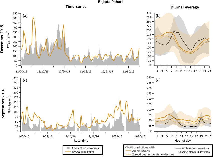
7726                                                                               B. Rooney et al.: Household sources of air pollution in India

Table 5. Mealtime∗ particulate matter surface emissions over a corresponding 16 km2 grid cell.

                                                         Bajada Pahari                    SOMAARTH HQ                              New Delhi
                                 Species            Total      % Residential            Total      % Residential             Total      % Residential
                                 POC                35.17                 67.13        36.04                    100        609.73               5.70
                                 PEC                10.22                 33.23         6.02                    100        346.84               2.21
                                 PCL                 2.19                   100         3.40                    100          3.40               100
                Particulate      PK                  0.43                  100          0.66                    100          0.66               100
                matter           PNA                 0.08                  100          0.12                    100          0.12               100
                (kg d−1 )        PNH4               1.037                   100         1.61                    100          1.61               100
                                 PNO3                0.37                 32.01         0.18                    100         12.59               1.45
                                 PSO4                2.49                  5.90         0.23                    100        116.80               0.20
                                 PMC                63.99                 91.94        72.56                    100        275.99               7.12
                                 PMOTHR             13.92                 61.94        13.37                    100        276.91               4.83
                SOA              NAPH               0.11                   6.50         0.03                  59.56         3.78                0.65
                precursor        SOAALK           112.31                  50.62       113.20                  77.95      1696.26               11.14
                VOCs             TOL               43.88                  42.28        39.38                  71.05       750.00                1.04
                (mol d−1 )       XYLMN             56.47                   6.50        13.03                  59.56      1886.15                0.65
              ∗ Mealtimes are assumed to be 04:00–10:00 and 16:00–20:00 (local time).

Table 6. Ambient observation data availability.

                                Location (grid cell)          PM2.5                                   O3
                                Bajada Pahari1                20–31 December 2015                     Not available
                                (74,74)                       19–30 September 16
                                SOMAARTH HQ1                  22–27 September 2015                    Not available
                                (75, 74)                      23–30 September 2016
                                West New Delhi2               7–30 September 2015                     7–30 September 2015
                                (71, 91)                      7–31 December 2015                      7–31 December 2015
                                                              7–30 September 2016
                                South New Delhi2              7–30 September 2015                     7–30 September 2015
                                (71, 89)                      7–31 December 2015                      7–31 December 2015
                                                              7–30 September 2016                     7–30 September 2016
                              1 Data from the International Epidemiological Clinical Network. Observations at Bajada Pahari are the
                              average of two monitoring locations that coincide within the same grid cell. 2 Data from the Central Pollution
                              Control Board of India at New Delhi Punjabi Bagh monitoring station.

tions from the NASA Goddard Earth Observing System Fast                                 Simulations were run for 1 year, after which hourly time
Processing (GEOS-FP) of the Global Modeling and Assim-                                  series diagnostics were compiled for the CMAQ modeling
ilation Office (GMAO), to simulate the boundary condi-                                  period. Using the PseudoNetCDF processor, we remapped a
tions for the CMAQ modeling. Simulations are performed                                  subset of the 616 GEOS-Chem-produced species to CMAQ
at 2◦ × 2.5◦ horizontal resolution with 72 vertical layers, in-                         species (https://github.com/barronh/pseudonetcdf, last ac-
cluding both the full tropospheric chemistry with complex                               cess: 28 May 2019). The resulting ICs and BCs include
SOA formation (Marais et al., 2016) and UCX stratospheric                               119 gas- and particle-phase species, 80 adapted from GEOS-
chemistry (Eastham et al., 2014). Emissions used the stan-                              Chem and the remaining 39 (including OH, HO2 , ROOH,
dard HEMCO configuration (Keller et al., 2014), including                               oligomerized secondary aerosols, coarse aerosol, and aerosol
EDGAR v4.2 anthropogenic emissions (http://edgar.jrc.ec.                                number concentration distributions) from the CMAQ default
europa.eu/overview.php?v=42, last access: 28 May 2019),                                 initial and boundary conditions data (which were developed
biogenic emissions from the MEGAN v2.1 inventory (Guen-                                 to represent typical clean-air pollutant concentrations in the
ther et al., 2012), and GFED biomass burning emissions                                  United States).
(http://www.globalfiredata.org, last access: 28 May 2019).

Atmos. Chem. Phys., 19, 7719–7742, 2019                                                                         www.atmos-chem-phys.net/19/7719/2019/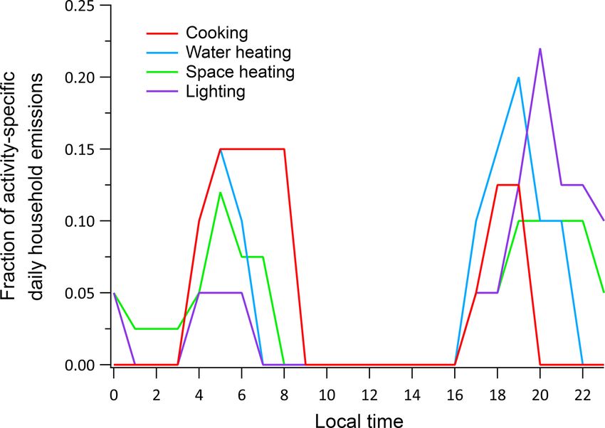
B. Rooney et al.: Household sources of air pollution in India                                                                                       7727

Table 7. Simulation durations.

                    CMAQ1                             7–30 September 2015            7–31 December 2015              7–30 September 2016
                    WRF2                              2–30 September 2015            2–31 December 2015              2–30 September 2016
                    (Meteorology)
                    GEOS-Chem3                        7–30 September 2015            7–31 December 2015              7–30 September 2016
                    (boundary conditions)
                  1 Five days prior to date shown were run and omitted from analysis as spinup. 2 One day prior to date shown was run and omitted
                  from analysis as spinup. 3 GEOS-Chem was run for 1 year before extracting atmospheric diagnostics.

3.2   Weather Research and Forecasting (WRF) model                                   carbons. Some organic compounds are apportioned based on
                                                                                     reactivity, and others, like isoprene, ethene, and formalde-
Three monthly WRF version 3.6.1 simulations were con-                                hyde, are treated explicitly.
ducted in the absence of nudging or data assimilation. The                              The secondary organic aerosol module, AERO6, devel-
large-scale forcing to generate initial and boundary me-                             oped specifically for CMAQ, interfaces with the gas-phase
teorological fields is adopted from the latest version of                            mechanism, predicts microphysical processes of emission,
the European Centre for Medium-Range Weather Forecasts                               condensation, evaporation, coagulation, new particle forma-
(ECMWF) ERA5 released in January 2019 (Copernicus Cli-                               tion, and chemistry, and produces a particle size distribu-
mate Change Services, 2017). These reanalysis data are on a                          tion comprising the sum of the Aitken, Accumulation, and
31 km grid and resolve the atmosphere using 137 levels from                          Coarse log-normal modes (Fig. 4). AERO6 predicts the for-
the surface to a height of 80 km. WRF simulations were per-                          mation of SOA from anthropogenic and biogenic VOC pre-
formed with 4 km horizontal resolution and 24 vertical lay-                          cursors (properties of which are shown in Table 8), as well
ers (the lowest layer of about 50 m depth), consistent with                          as semivolatile POA and cloud processes. CB6R3 accounts
the setup of the CMAQ model. No cumulus parameterization                             for the oxidation of the first-generation products of the an-
was used in the simulations. Meteorological outputs from                             thropogenic lumped VOCs: high-yield aromatics, low-yield
WRF were prepared as inputs to CMAQ by the Meteorology-                              aromatics, benzene, PAHs, and long-chain alkanes (Pye and
Chemistry Interface Processor (MCIP) version 4.4 (Otte et                            Pouliot, 2012).
al., 2010).                                                                             In addition to SOA formation from traditional precursors,
                                                                                     CMAQv5.2 accounts for the semivolatile partitioning and
3.3   Community Multiscale Air Quality (CMAQ)                                        gas-phase aging of POA using the volatility basis set (VBS)
      modeling system                                                                framework independently from the rest of AERO6 (Mur-
                                                                                     phy et al., 2017). The module distributes directly emitted
Within the chemical transport portion of CMAQ, there are                             POA (as the sum of primary organic carbon, POC, and non-
two primary components: a gas-phase chemistry module and                             carbon organic matter, NCOM) from the emissions inven-
an aerosol chemistry, gas-to-particle conversion module. The                         tory input into five new emitted species grouped by volatil-
present study employs a CMAQ-adapted gas-phase chem-                                 ity: LVPO1, SVPO1, SVPO2, SVPO3, and IVPO1 (where
ical mechanism, CB6R3 (derived from the Carbon Bond                                  LV is low volatility, SV is semivolatile, IV is intermediate
Mechanism 06) (Yarwood et al., 2010), and the aerosol-                               volatility, and PO is primary organic). POA is apportioned to
phase mechanism, AERO6, which define the gas-phase and                               these lumped vapor species using an emission fraction and
aerosol-phase chemical resolution. The present study con-                            is oxidized in CB6R3 by OH to LVOO1, LVOO2, SVOO1,
siders 70 NMHC compounds lumped into 12 groups of                                    SVOO2, and SVOO3 (where OO denotes oxidized organ-
VOCs. The emissions inventory provides emission rates for                            ics) with stoichiometric coefficients derived from the 2D-
28 chemical species, including 18 gas-phase species and 10                           VBS model. AERO6 then partitions the semivolatile primary
particle-phase species. The CB6R3 adaptation describes at-                           organics and their oxidation products to the aerosol phase
mospheric oxidant chemistry with 127 gas-phase species and                           (Fig. 4). Thus, the treatment of POA as semivolatile prod-
220 gas-phase reactions, including chlorine and heteroge-                            ucts leads to an additional twenty species, a particle- and
nous reactions. The CMAQ aerosol module (AERO6) de-                                  vapor-phase component for each primary organic and oxi-
scribes aerosol chemistry and gas-to-particle conversion with                        dation product (Murphy et al., 2017).
12 traditional SOA precursor classes, and 10 semivolatile pri-                          Emissions inventory modifications were required to match
mary organic aerosol (POA) precursor reactions. The ma-                              the most recent aerosol module, AERO6, in the CMAQ
jority of the gas-phase organic species are apportioned to                           model. Initially, the lumped emissions of PAR (a lumped
lumped groups by their carbon bond characteristics, such as                          VOC group characterized by alkanes) and XYL (a lumped
single bonds, double bonds, ring structure, and number of                            VOC group characterized by xylene) derived from grouping

www.atmos-chem-phys.net/19/7719/2019/                                                                       Atmos. Chem. Phys., 19, 7719–7742, 2019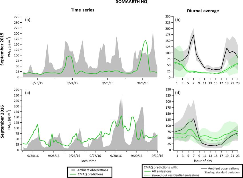
7728                                                                                B. Rooney et al.: Household sources of air pollution in India

Figure 4. Treatment of anthropogenic SOA in CMAQv5.2. Predicted aerosol species are included in the black box. Species in white boxes are
semivolatile and species in gray boxes are nonvolatile. Blue indicates species and processes predicted by CB6R3. All other coloring indicates
the AERO6 mechanism where green arrows are two-product volatility distribution, orange arrows are particle- and vapor-phase partitioning,
and purple arrows are oligomerization. In AERO6, anthropogenic and biogenic VOC emissions (lumped by category) are oxidized by OH,
NO, and HO2 and OH, O3 , NO, and NO3 respectively, to semivolatile products that undergo partitioning to the particle phase (Pye et al.,
2015). Semivolatile primary organic pathways in CMAQv5.2 are described by Murphy et al. (2017).

Table 8. Properties of anthropogenic traditional semivolatile SOA precursors in CMAQv5.2. NA denotes not applicable.

                                                                                     α                                                  Molecular
     SOA                                                      Semi-              (mass-           C∗             1Hvap          No.        weight
     species       Precursor                  Oxidants        volatile           based)      (µg m−3 )       (kJ mol−1 )       of C     (g mol−1 )       OM / OC
     AALK1         long-chain alkanes         OH              SV_ALK1           0.0334             0.15              53.0        12             168            1.17
     AALK2         long-chain alkanes         OH              SV_ALK2           0.2164             51.9              53.0        12             168            1.17
     AXYL1         XYLMN                      OH, NO          SV_XYL1           0.0310              1.3              32.0         8             192             2.0
     AXYL2         XYLMN                      OH, NO          SV_XYL2           0.0900             34.5              32.0         8             192             2.0
     AXYL3         XYLMN                      OH, HO2         nonvolatile         0.36              NA                NA        NA              192             2.0
     ATOL1         TOL                        OH, NO          SV_TOL1           0.0310              2.3              18.0         7             168             2.0
     ATOL2         TOL                        OH, NO          SV_TOL2           0.0900             21.3              18.0         7             168             2.0
     ATOL3         TOL                        OH, HO2         nonvolatile         0.30              NA                NA        NA              168             2.0
     ABNZ1         benzene                    OH, NO          SV_BNZ1           0.0720             0.30                18         6             144             2.0
     ABNZ2         benzene                    OH, NO          SV_BNZ2           0.8880              111                18         6             144             2.0
     ABNZ3         benzene                    OH, HO2         nonvolatile         0.37              NA                NA        NA              144             2.0
     APAH1         naphthalene                OH, NO          SV_PAH1           0.2100             1.66                18        10             243            2.03
     APAH2         naphthalene                OH, NO          SV_PAH2           1.0700              265                18        10             243            2.03
     APAH3         naphthalene                OH, HO2         nonvolatile         0.73              NA                NA        NA              243            2.03
   The semivolatile reaction products of “long alkanes” (SV_ALK1 and SV_ALK2) are parameterized by Presto et al. (2010). Values for “low-yield aromatics” products
   (SV_XYL1 and SV_XYL2) are based on xylene, with the enthalpy of vaporization (1Hvap ) from studies of m-xylene and 1,3,5-trimethylbenzene. 1Hvap for products of
   “high-yield aromatics” (SV_TOL1 and SV_TOL2) are based on the higher end of the range for toluene. The products of benzene (SV_BNZ1 and SV_BNZ2) assume the
   same value for 1Hvap . All semivolatile aromatic products are assigned stoichiometric yield (α ) and effective saturation concentration (C∗ ) values from laboratory
   measurements by Ng et al. (2007). Remaining parameters for PAH reaction products (SV_PAH1 and SV_PAH2) are taken from Chan et al. (2009). Properties of
   semivolatile primary organic aerosol precursors are given in Murphy et al. (2017).

Atmos. Chem. Phys., 19, 7719–7742, 2019                                                                        www.atmos-chem-phys.net/19/7719/2019/
B. Rooney et al.: Household sources of air pollution in India 7729
Figure 5. Evaluation of WRF-simulated meteorological fields versus ground observations.
Table 9. Quantification of WRF model biases in meteorological fields.
Bajada Pahari SOMAARTH HQ West New Delhi South New Delhi
Sep 15 Dec 15 Sep 16 Sep 15 Dec 15 Sep 16 Sep 15 Dec 15 Sep 16 Sep 15 Dec 15 Sep 16
PRE – 15.28 30.10 29.27 – 30.22 30.45 16.59 30.07 30.32 17.59 29.96
(4.59) (3.19) (3.48) (3.06) (3.79) (4.91) (3.05) (3.74) (4.82) (30.3)
Temperature OBS – 15.62 30.86 32.15 – 33.26 32.80 19.04 31.46 28.48 12.58 29.22
(◦ C) (4.91) (5.67) (4.12) (5.31) (3.60) (3.66) (2.33) (4.30) (5.52) (4.22)
MB – −0.34 −0.76 −2.89 – −3.04 −2.35 −2.45 −1.38 1.84 5.02 0.74
ME – 1.60 3.08 2.92 – 3.07 3.03 2.58 1.54 2.11 5.02 2.37
RMSE – 2.20 3.71 3.39 – 3.99 3.58 2.99 1.88 2.50 5.33 2.75
PRE – 2.91 2.31 – – 2.01 – – 2.57 2.80 2.72 2.74
(1.17) (1.07) (0.66) (1.28) (1.27) (1.08) (1.39)
Wind OBS – 1.18 0.73 – – 0.55 – – 1.03 1.26 0.94 1.18
speed (0.75) (0.40) (0.30) (0.51) (0.83) (0.71) (0.79)
(m s−1 ) MB – 1.72 1.58 – – 1.46 – – 1.54 1.54 1.77 1.56
ME – 1.75 1.62 – – 1.50 – – 1.58 1.61 1.82 1.62
RMSE – 1.96 1.85 – – 1.66 – – 1.88 1.85 2.01 1.84
PRE – 247 116 272 – 111 – – 179 206 254 191
(111) (45) (70) (51) (98) (118) (97) (96)
Wind OBS – 259 102 255 – 110 – – 181 198 224 228
direction (57) (41) (58) (48) (97) (45) (44) (50)
(◦ ) MB – 0.14 14 16 – −0.14 – – -6 9 35 −34
ME – 51 38 44 – 32.71 – – 49 94 74 75
RMSE – 66 51 64 – 47.50 – – 64 106 87 90
PRE is mean predictions. OBS is mean observations. MB is mean bias. ME is mean error. and RMSE is root mean square error. Standard deviation of predictions and observations are noted in
parentheses.
specific NMHCs, calculated using the University of Illinois dicts the formation of SOA from NAPH and SOAALK in-
estimation and the Fleming et al. (2018a) emission factors, dependently as well as from XYL and PAR; these secondary
accounted for characteristics of naphthalene (NAPH) and aerosol precursor emission rates are calculated with the fol-
SOA-producing alkanes (SOAALK), which are not individu- lowing:
ally described by any of the sources used to construct the in-
ventory. Moreover, only a subset of VOCs in the plume could XYLMN = 0.998 × XYL, (3)
be measured. However, CMAQv5.2 simulations incorporate NAPH = 0.002 × XYL, (4)
a surrogate species, potential secondary organic aerosol from PARCMAQ = PARcalculated − 0.00001 × NAPH, (5)
combustion emissions (pcSOA), to address sources of miss-
ing SOA, including unspeciated emissions of semivolatile SOAALK = 0.108 × PARCMAQ , (6)
and intermediate volatility organic compounds. AERO6 pre-
www.atmos-chem-phys.net/19/7719/2019/ Atmos. Chem. Phys., 19, 7719–7742, 20197730 B. Rooney et al.: Household sources of air pollution in India
Figure 6. Measured and predicted PM2.5 (a, c) and average diurnal cycle (b, d) in Bajada Pahari for 20–31 December 2015 (a, b) and
20–30 September 2016 (c, d). Here the yellow lines correspond to CMAQ predictions of the “total” (solid) and “nonresidential” (dotted)
simulations. The solid black line represents ambient observations. Standard deviations of the diurnal profiles for observations and predictions
are indicated, respectively, by colored shading. Diurnal profiles were averaged over simulation durations (Table 7). Computations were
carried out at 4 km resolution.
where XYLMN, NAPH, PARCMAQ , and SOAALK are SOMAARTH HQ). Ambient measurement sites are shown
the new inventory species (Pye and Pouliot, 2012). SOA- in Fig. 1, and Table 6 details available data for each location.
producing alkanes are treated separately in AERO6. We used meteorological data (hourly surface temperature and
near-surface wind speed and direction) from INCLEN and
CPCB at the two rural and two urban sites, respectively, to
4 Surface observational data evaluate the WRF simulations performance.
Gas-phase air quality data analyzed in the present study come
from the Central Pollution Control Board (CPCB) of the
Ministry of Environment, Forest & Climate Change of the 5 Simulation results
Government of India at two sites in New Delhi (one in the
west, and one in the south) (CPCB, 2019). The particle- 5.1 WRF evaluation
phase data analyzed come from the SOMAARTH Demo-
graphic, Development, and Environmental Surveillance Site We evaluated WRF-simulated meteorology against the avail-
(Mukhopadhyay et al., 2012; Pillarisetti et al., 2014; Balakr- able surface observations at different sites during the same
ishnan et al., 2015) managed by INCLEN. Palwal District has periods. Figure 5 shows that there is generally good agree-
a population of ∼ 1 million over an area of 1400 km2 . In this ment in surface temperature between WRF and observations
district, ∼ 39 % of households utilize wood burning as their for all three months. The surface wind direction is found to
primary cooking fuel, with dung (∼ 25 %) and crop residues be consistent between model and observations for each site
(∼ 7 %) (Census of India, 2011). The specific sites studied and each month (Table 9). The simulated near-surface wind
are the SOMAARTH HQ in Aurangabad (15 km south of speeds are overestimated in WRF, with an averaged mean
Palwal) and the village of Bajada Pahari (8 km northwest of bias (MB) of about +1.5 m s−1 . Such a bias is partly a result
Atmos. Chem. Phys., 19, 7719–7742, 2019 www.atmos-chem-phys.net/19/7719/2019/B. Rooney et al.: Household sources of air pollution in India 7731
Figure 7. Measured and predicted PM2.5 (a, c) and average diurnal cycle (b, d) at SOMAARTH HQ for 20–31 December 2015 (a, b) and
20–30 September 2016 (c, d). Here the green lines correspond to CMAQ predictions of the “total” (solid) and “nonresidential” (dotted) sim-
ulations. The solid black line represents ambient observations. Standard deviations of the diurnal profiles for observations and predictions are
indicated by gray and green colored shading, respectively. Diurnal profiles were averaged over simulation durations (Table 7). Computations
were carried out at 4 km resolution.
of the difference in the definition of “near-surface” between hari in December 2015 and September 2016, SOMAARTH
the model and observations. HQ in September 2015 and 2016, West New Delhi in Decem-
ber 2015, and South New Delhi in December and Septem-
5.2 Particulate matter ber 2015. Average daily PM2.5 levels regularly exceed the
24 h Indian standard of 60 µg m−3 in each month in both rural
Figures 6–9 show measured and predicted total PM2.5 and and urban locations, surpassing even double the standard in
the average diurnal profile at each site for the periods with the village of Bajada Pahari during mealtimes in December.
available measurements. The diurnal profile in these fig- Afternoon minima tend to be underestimated in September
ures includes that of both emission scenarios: the total sce- and December 2015. Diurnal trends of PM2.5 were weaker
nario with all emissions and the nonresidential scenario with in September 2016 than the other months, with lower pre-
zeroed-out residential sector. The simulations capture the dictions but overestimated minima. Urban sites show greater
general trend well and produce significant diurnal profiles overestimation than rural sites. This is likely due in part to the
(Table 10). Rural sites show typical PM2.5 levels are pre- granularity of the primary emissions inventory datasets. The
dicted between 50 and 125 µg m−3 in December and 25 and nonresidential sector was prepared from data with a native
75 µg m−3 in September months (Figs. 6 and 7). On the resolution of 36 km, while the residential sector used data
other hand, typical values at urban sites range from 100 to with ∼ 1 km resolution. Underpredictions of peak PM2.5 con-
300 µg m−3 in December and 50 to 125 µg m−3 in Septem- centrations in September could also result because the emis-
ber months (Figs. 8 and 9). Observations and predictions sion inventory does not account for day-to-day variations, es-
show higher PM2.5 levels in December than September, ow- pecially in the agricultural burning sector in which emissions
ing to frequent temperature inversions in winter and shal- can change significantly on a daily basis. Observed and pre-
lower planetary boundary layers. Two daily peaks and lows dicted PM2.5 levels in New Delhi can exceed 300 µg m−3 ,
of PM2.5 compare with ambient observations at Bajada Pa-
www.atmos-chem-phys.net/19/7719/2019/ Atmos. Chem. Phys., 19, 7719–7742, 20197732 B. Rooney et al.: Household sources of air pollution in India
Figure 8. Measured and predicted PM2.5 (a, c) and average diurnal cycle (b, d) in West New Delhi for 20–31 December 2015 (a, b) and
20–30 September 2016 (c, d). Here the pink lines correspond to CMAQ predictions of the “total” (solid) and “nonresidential” (dotted) simu-
lations. The solid black line represents ambient observations. Standard deviations of the diurnal profiles for observations and predictions are
indicated by gray and pink colored shading, respectively. Diurnal profiles were averaged over simulation durations (Table 7). Computations
were carried out at 4 km resolution.
especially in winter. In this highly populated urban environ- stations is nearly double that of September 2016, which can
ment, particulate matter levels are more than double those re- be attributed to temperature inversions and a shallower plan-
ported in the nearby rural areas. The employed emissions in- etary boundary layer in winter.
ventory specifies particulate matter surface emissions, which The significance of household emissions on outdoor PM2.5
surpass those of Bajada Pahari and SOMAARTH HQ more concentrations is demonstrated by the diurnal profiles in
than 30-fold (Table 5). Biogenic emissions are predicted to Fig. 11. Figure 11a, b, and c the predicted contribution of
be of little importance, accounting for less than 10 % on av- the residential sector to anthropogenic PM2.5 , while Fig. 11
erage of total PM2.5 concentrations for most stations and d, e, and f describe the predicted contribution of the residen-
months (Table 10). tial sector to secondary organic PM2.5 , as in Eqs. (7) and (8)
Figure 10 shows CMAQ predictions of secondary organic respectively:
PM2.5 (SOA). Like PM2.5 , SOA is typically predicted to be
higher in New Delhi than in the rural sites, due to higher Residential anthropogenic PM2.5
, (7)
PM2.5 and precursor VOC emissions and ambient concentra- Total anthropogenic PM2.5
tions in urban environments (Tables 5 and 6). Higher lev-
els are similarly attained in December than in September
due to longer residence times and more aging during win- Residential SOA
. (8)
ter. SOA has high day-to-day variability. Values range from Total SOA
below 20 µg m−3 to over 200 µg m−3 in December, with av- Figure 11g, h, and i show the predicted SOA portion of resi-
erage peaks up to 55 µg m−3 at the rural sites. September dential PM2.5 , as
months predict lower SOA, ranging from 10 to 130 µg m−3 .
Diurnal average SOA maximum in December for the rural Residential SOA
, (9)
Residential PM2.5
Atmos. Chem. Phys., 19, 7719–7742, 2019 www.atmos-chem-phys.net/19/7719/2019/B. Rooney et al.: Household sources of air pollution in India 7733 Figure 9. Measured and predicted PM2.5 (a, c, e) and average diurnal cycle (b, d, f) in South New Delhi for 20–31 December 2015 (a, b) and 20–30 September 2016 (c–f). Here the blue lines correspond to CMAQ predictions of the “total” (solid) and “nonresidential” (dotted) simu- lations. The solid black line represents ambient observations. Standard deviations of the diurnal profiles for observations and predictions are indicated by gray and blue colored shading, respectively. Diurnal profiles were averaged over simulation durations (Table 7). Computations were carried out at 4 km resolution. where residential PM is calculated as the difference in pre- ior is predicted for SOA (Fig. 11b, e, and h). An estimated dictions from the nonresidential and total emission scenario 15 % to 34 % of secondary organic matter is attributable to and averaged over simulation durations (Table 7). The im- residential emissions in September and 2016. Again, the im- portance of household emissions to ambient PM is strongly pact is smaller in West and South New Delhi (up to 19 % correlated with mealtimes. Predicted maximum contributions and 21 %, respectively in September 2016), where there are to anthropogenic PM2.5 in Bajada Pahari and SOMAARTH greater emissions of SOA precursors from other sectors. The HQ are about double that of South and West New Delhi for diurnal profile of the contribution to SOA is subdued for all each month. Household energy use is estimated to account sites in December, suggesting that SOA generation is less ef- for up to 27 % of anthropogenic PM2.5 (at SOMAARTH ficient in winter when radiation and temperatures are lower. HQ during September 2016), remaining consistently above The aging of VOCs is captured by the phase shift of the im- 10 % for each rural site during all months. Similar behav- pact on SOA daily trend, where peaks consistently occur an www.atmos-chem-phys.net/19/7719/2019/ Atmos. Chem. Phys., 19, 7719–7742, 2019
7734                                                                                                   B. Rooney et al.: Household sources of air pollution in India

Table 10. CMAQ model performance and summary statistics.

                                             Bajada Pahari                         SOMAARTH HQ                                  West New Delhi                             South New Delhi
                                 Dec 15         Sep 15        Sep 16        Dec 15         Sep 15        Sep 16        Dec 15          Sep 15        Sep 16        Dec 15         Sep 15        Sep 16
                   PRE          133.49            54.83        59.22        131.80          32.16          63.66       212.29         101.71        106.44         191.35           92.68         92.85
                                (40.66)         (21.24)       (9.89)        (42.81)       (15.99)        (11.24)       (75.55)        (41.49)       (28.58)        (61.03)        (39.46)       (24.37)
                   OBS          136.01                –        35.55              –         75.83          58.03       120.49           81.53             –        254.15           70.24         70.97
   PM2.5                        (28.35)               –      (13.76)              –       (37.16)        (35.19)       (29.92)        (12.72)             –        (70.89)        (13.04)       (18.72)
                   MB            −2.52                –        23.67              –       −43.67            5.64         91.80          20.19             –        −62.81           22.44         21.88
                   ME             35.20               –        24.66              –         43.67          25.04         91.93          41.02             –          67.67          26.42         25.71
                   RMSE           40.23               –        26.35              –         56.23          27.71       115.76           48.60             –          81.02          37.50         35.37
                   PRE            72.76           80.72        47.24          71.83         80.75          47.22         32.59          57.14         31.66          40.90          62.76         36.29
                                (39.47)          (3.87)      (17.56)        (39.99)       (34.06)        (17.60)       (41.34)        (53.36)       (30.16)        (44.87)        (53.52)       (29.89)
                   OBS                –               –            –              –             –              –         21.74          71.09             –          43.57          59.47         29.28
   O3                                                                                                                   (8.05)        (42.41)                      (37.07)        (36.30)       (20.27)
                   MB                    –             –             –              –              –             –       10.93        −13.95                –       −2.67            3.29          7.01
                   ME                    –             –             –              –              –             –       16.83          18.74               –        12.62          24.72         19.29
                   RMSE                  –             –             –              –              –             –       22.96          22.10               –        14.08          27.64         23.31
                   PRE            44.60           17.89        23.30         44.81          18.06         22.95          44.22          23.76         33.28          43.95         22.44          31.78
   SOA
                                  (7.76)         (2.40)        (3.96)        (7.59)         (2.34)        (3.77)         (3.76)         (4.74)        (8.80)         (3.82)        (4.11)         (7.84)
                   PRE              0.09           0.18          0.08          0.09           0.18          0.08           0.04           0.06          0.04           0.04          0.03           0.05
   Fbio
                                  (0.03)         (0.10)        (0.02)        (0.03)         (0.11)        (0.02)         (0.01)         (0.01)        (0.01)         (0.01)        (0.01)         (0.01)
                   PRE              0.15           0.24          0.26          0.15           0.24          0.26           0.13           0.15          0.16           0.13          0.16           0.16
   FSOA,res
                                  (0.02)         (0.05)        (0.04)        (0.02)         (0.05)        (0.04)         (0.03)         (0.02)        (0.03)         (0.03)        (0.02)         (0.03)
                   PRE              0.12           0.16          0.20          0.12           0.17          0.20           0.07           0.08          0.09           0.07          0.08           0.10
   Fan,res
                                  (0.03)         (0.04)        (0.03)        (0.03)         (0.04)        (0.04)         (0.02)         (0.03)        (0.02)         (0.02)        (0.03)         (0.02)
                   PRE              0.48           0.51          0.52          0.47           0.50          0.52           0.43           0.51          0.55           0.45          0.53           0.54
   Fres,SOA
                                  (0.16)         (0.20)        (0.18)        (0.16)         (0.21)        (0.18)         (0.18)         (0.21)        (0.17)         (0.18)        (0.22)         (0.17)
 Statistics are calculated for average diurnal profiles of predicted parameters. PM2.5 , O3 , and SOA are the mass concentrations in micrograms per cubic meter (µg m−3 ) of total fine particulate
 matter, ozone, and secondary organic matter, respectively. Fbio is the fraction of total PM2.5 that is produced by biogenic emissions, FSOA,res is the fraction of total secondary organic matter
 attributable to the residential sector, Fan,res is the fraction of total anthropogenic PM2.5 attributable to the residential sector, and Fres,SOA is the fraction of residential PM2.5 attributable to SOA.
 PRE is mean predictions, OBS is mean observations, MB is mean bias, ME is mean error, and RMSE is root mean square error. Standard deviation of predictions and observations are noted in
 parentheses.

hour after the residential sector shows the greatest impor-                                                versity of energy-use activities and emissions characteristics
tance to anthropogenic PM2.5 .                                                                             in the urban environment.
   At each measurement site during all months, SOA is pre-
dicted to make up more than 40 % of PM2.5 produced by                                                      5.3       Ozone
the residential sector on average (Fig. 11g–i). SOA is least
significant to residential PM2.5 in the first half of mealtimes                                            The 8 h India Central Pollution Control Board (CPCB) stan-
(∼ 20 % during breakfast and ∼ 40 % during dinner) at rural                                                dard for ozone is 100 µ m−3 for an 8 h average. In the alter-
sites, when primary particulate matter is largest. The aging of                                            native unit of ozone mixing ratio, a mass concentration of
precursor VOCs from cooking emissions, paired with maxi-                                                   ozone of 100 µg m−3 at a temperature of 298 K at the Earth’s
                                                  Residential SOA
mum incoming radiation, leads to maximum Residential                                                       surface equates to a mixing ratio of 51 parts per billion (ppb).
                                                             PM2.5
values in early afternoon, when SOA accounts for more than                                                 A number of atmospheric modeling studies of ozone over In-
75 % of residential PM2.5 at both rural and urban sites during                                             dia exist (Kumar et al., 2010; Chatani et al., 2014; Sharma et
each simulated month.                                                                                      al., 2016).
   The fractional contribution of total SOA to total PM2.5 is                                                 Sharma et al. (2016) carried out baseline CMAQ simula-
shown in Fig. 12. While concentrations of SOA depend sig-                                                  tions for 2010 and compared ozone predictions with mea-
nificantly on the site and time period, their contribution to                                              surements at six monitoring locations in India (Thumba,
total PM2.5 shows little variation. At all stations, SOA is pre-                                           Gādanki, Pune, Anantpur, Mt. Abu, and Nainital). Also car-
dicted to make up to 55 % of PM2.5 in September months and                                                 ried out were sensitivity simulations in which each emis-
to be most significant around midday. However, diurnal vari-                                               sions sector (transport, domestic, industrial, power, etc.) was
ation of the significance of SOA is greater in New Delhi than                                              systematically set to zero. The domestic sector was pre-
in Bajada Pahari or SOMAARTH HQ, owing to greater di-                                                      dicted to contribute ∼ 60 % of the nonmethane volatile or-
                                                                                                           ganic carbon emissions, followed by 12 % from transporta-
                                                                                                           tion and 20 % from solvent use and the oil and gas sector. The

Atmos. Chem. Phys., 19, 7719–7742, 2019                                                                                               www.atmos-chem-phys.net/19/7719/2019/
You can also read