Comparison of root water uptake models in simulating CO2 and H2O fluxes and growth of wheat - HESS
←
→
Page content transcription
If your browser does not render page correctly, please read the page content below
Hydrol. Earth Syst. Sci., 24, 4943–4969, 2020
https://doi.org/10.5194/hess-24-4943-2020
© Author(s) 2020. This work is distributed under
the Creative Commons Attribution 4.0 License.

Comparison of root water uptake models in simulating CO2
and H2O fluxes and growth of wheat
Thuy Huu Nguyen1 , Matthias Langensiepen1 , Jan Vanderborght3 , Hubert Hüging1 , Cho Miltin Mboh4 , and
Frank Ewert1,2
1 Universityof Bonn, Institute of Crop Science and Resource Conservation (INRES),
Katzenburgweg 5, 53115 Bonn, Germany
2 Leibniz Centre for Agricultural Landscape Research (ZALF), Institute of Landscape Systems Analysis,

Eberswalder Strasse 84, 15374 Muencheberg, Germany
3 Agrosphere, Institute of Bio- and Geosciences (IBG-3), Forschungszentrum Jülich GmbH, 52428 Jülich, Germany
4 BASF Digital Farming GmbH, Im Zollhafen 24, 50678 Cologne, Germany

Correspondence: Thuy Huu Nguyen (tngu@uni-bonn.de)

Received: 21 April 2020 – Discussion started: 4 May 2020
Revised: 5 August 2020 – Accepted: 4 September 2020 – Published: 23 October 2020

Abstract. Stomatal regulation and whole plant hydraulic sig-       of dry matter, leaf area index (LAI), root growth, RWU,
naling affect water fluxes and stress in plants. Land sur-         gross assimilation rate, and soil water content. The Feddes
face models and crop models use a coupled photosynthesis–          model predicts more stress and less growth in the silty soil
stomatal conductance modeling approach. Those models es-           than in the stony soil, which is opposite to the observed
timate the effect of soil water stress on stomatal conductance     growth. The Couvreur model better represents the difference
directly from soil water content or soil hydraulic potential       in growth between the two soils and the different treatments.
without explicit representation of hydraulic signals between       The newly coupled model (HILLFLOW–Couvreur’s RWU–
the soil and stomata. In order to explicitly represent stom-       SLIMROOT–LINTULCC2) was also able to simulate the dy-
atal regulation by soil water status as a function of the hy-      namics and magnitude of whole plant hydraulic conductance
draulic signal and its relation to the whole plant hydraulic       over the growing season. This demonstrates the importance
conductance, we coupled the crop model LINTULCC2 and               of two-way feedbacks between growth and root water up-
the root growth model SLIMROOT with Couvreur’s root                take for predicting the crop response to different soil water
water uptake model (RWU) and the HILLFLOW soil wa-                 conditions in different soils. Our results suggest that a bet-
ter balance model. Since plant hydraulic conductance de-           ter representation of the effects of soil characteristics on root
pends on the plant development, this model coupling rep-           growth is needed for reliable estimations of root hydraulic
resents a two-way coupling between growth and plant hy-            conductance and gas fluxes, particularly in heterogeneous
draulics. To evaluate the advantage of considering plant hy-       fields. The newly coupled soil–plant model marks a promis-
draulic conductance and hydraulic signaling, we compared           ing approach but requires further testing for other scenarios
the performance of this newly coupled model with another           regarding crops, soil, and climate.
commonly used approach that relates root water uptake and
plant stress directly to the root zone water hydraulic potential
(HILLFLOW with Feddes’ RWU model). Simulations were
compared with gas flux measurements and crop growth data           1   Introduction
from a wheat crop grown under three water supply regimes
(sheltered, rainfed, and irrigated) and two soil types (stony      Soil water status is amongst the key factors that influence
and silty) in western Germany in 2016. The two models              photosynthesis, evapotranspiration, and growth processes
showed a relatively similar performance in the simulation          (Hsiao, 1973). Accurate estimation of crop water stress re-
                                                                   sponses is important for predictions of crop growth, yield,

Published by Copernicus Publications on behalf of the European Geosciences Union.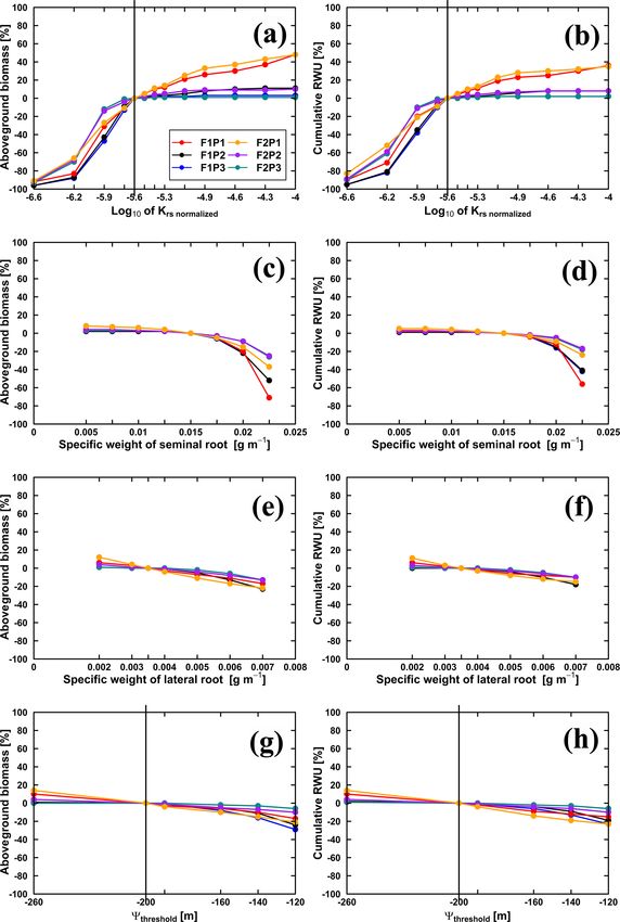
4944                     T. H. Nguyen et al.: Comparison of root water uptake models in simulating CO2 and H2 O fluxes

and water use by crop models and land surface models (Egea          linear soil water balance partial differential equation. It uses
et al., 2011).                                                      a stomatal regulation model that assumes that stomatal con-
   Crop models and land surface models lump the effects of          ductance is not influenced by the leaf water hydraulic head
soil water deficit on stomatal regulation and crop growth in        as long as the leaf hydraulic head is above a critical leaf
so-called “stress factors” (Verhoef and Egea, 2014; Mahfouf         hydraulic threshold. The leaf water hydraulic head is kept
et al., 1996). Crop water stress is strongly influenced by soil     constant by changing stomatal conductance when the criti-
water availability, which in turn depends on the distribution       cal leaf hydraulic threshold is reached. The Couvreur model
of water and of roots in the root zone and the transpiration        also allows the different stomatal regulations to be presented
rate or total root water uptake. Adequate representations in        (i.e., isohydric and anisohydric in Tardieu and Simonneau,
simulation models of root water uptake (hereafter RWU) and          1998) (Couvreur et al., 2014, 2012).
root distributions (Gayler et al., 2013; Wöhling et al., 2013;         Recently, inverse modeling routines using datasets of root
Zeng et al., 1998; Desborough, 1997) are therefore needed.          density, leaf area, and soil water content and potential per-
Most macroscopic RWU models estimate the water uptake as            mitted the quantification of root-related parameters of Cou-
a function of potential transpiration (i.e., the transpiration of   vreur’s model (root hydraulic conductivity). Sap flow mea-
the crop when water is not limited) and average moisture con-       surements were used to validate simulated RWU using the
tent or soil water pressure head and rooting densities (Feddes      parameterized model (Cai et al., 2017, 2018). These stud-
et al., 2001; van Dam, 2000). However, in this representa-          ies demonstrated the close relation between the root system
tion of RWU, crucial relations between RWU model param-             conductance and root growth as part of overall plant growth
eters and root and plant hydraulic conductances, which trans-       and its response to water stress pointing at a two-way cou-
late the soil water pressure head to water hydraulic heads          pling between root water uptake and plant growth. This im-
in the shoot to which stomata respond, are lost. Note that          plies that the parameterization of root water uptake needs to
hydraulic heads refer to total water potentials expressed in        be coupled to plant growth, which in turn is influenced by
length units and pressure heads to the hydraulic head minus         water stress and other factors. Plant hydraulic conductance
the gravitational potential or elevation. For instance, the wa-     was introduced in crop models for several field crops such
ter stress factor calculated by the Feddes model (Feddes et         as soybean (Olioso et al., 1996) and winter wheat (Wang et
al., 1978) based on the soil water pressure heads involves in-      al., 2007) or for model testing (Tuzet et al., 2003). However,
direct linkages between the root zone water pressure head           plant hydraulic conductance in these studies was kept con-
and the hydraulic head in the shoot in the sense that the           stant without reference to dynamic root growth. To the best
water stress factors are adapted when the potential transpi-        of our knowledge, the effect of two-way coupling between a
ration rate changes. Such models like the Feddes approach           RWU model accounting for whole plant hydraulic regulation
represent the role of the root and plant hydraulic conduc-          and a crop growth model has not been studied yet. It is un-
tance indirectly and thus require calibration for different crop    clear whether such a coupled model improves the simulation
types and growing seasons (Cai et al., 2018; Vandoorne et al.,      of crop growth and development and CO2 and H2 O fluxes.
2012; Wesseling et al., 1991). The conductance of the root             In this study, we coupled Couvreur’s RWU model (Cou-
system is an important feature of the root system and differ-       vreur et al., 2012, 2014) with the existing crop growth model
ent approaches to include it in RWU models were published           LINTULCC2 (Rodriguez et al., 2001) to consider the whole
(Quijano and Kumar, 2015; Vadez, 2014, Kramer and Boyer,            plant hydraulic conductance from root to shoot. The dynam-
1995; Peterson and Steudle, 1993). Plant hydraulic conduc-          ics of root and shoot growth under varying soil water avail-
tance determines leaf water potentials which have a signif-         ability are explicitly represented by the coupled model. The
icant impact on stomatal conductance, leaf gas exchange,            overall aim of the study was to investigate whether consider-
and leaf growth (Tardieu et al., 2014; Trillo and Fernández,        ation of plant hydraulic conductance can improve the simu-
2005; Sperry, 2000; Zhao et al., 2005; Gallardo et al., 1996).      lation of CO2 and H2 O fluxes and crop growth in biomass,
Recently, some one-dimensional macroscopic RWU models               roots, and leaf area index of the same crop that is grown
based on hydraulic principles have been developed to repre-         in two different soils and for three different water applica-
sent water potential gradients from the soil to roots (de Jong      tion regimes. To achieve this aim, three objectives were ad-
van Lier et al., 2008) and within the root system (Couvreur et      dressed: (i) to analyze and compare the predictive quality
al., 2014). The latter approach simplified a physically based       of a crop growth model coupled with a RWU model that
description of water flow in the coupled soil–root system ac-       considers plant hydraulics (Couvreur RWU model) and a
counting for the root system hydraulic properties and archi-        model that does not consider plant hydraulics (Feddes RWU
tecture to simple linear equations between soil water pressure      model); (ii) to compare the simulated plant hydraulic con-
heads, the leaf water hydraulic head, root water uptake pro-        ductances for the different growing conditions with direct
files, and the transpiration rate that can be solved directly.      estimates of these conductances from measurements; and
It thereby avoids computation of time-consuming numerical           (iii) to analyze the sensitivity of RWU and crop growth to
solutions of ordinary differential equations for the water flow     the Couvreur RWU and root growth model parameters (root
and balance in the root system that are coupled with the non-

Hydrol. Earth Syst. Sci., 24, 4943–4969, 2020                                        https://doi.org/10.5194/hess-24-4943-2020
T. H. Nguyen et al.: Comparison of root water uptake models in simulating CO2 and H2 O fluxes                                 4945

hydraulic conductance, critical leaf hydraulic threshold, and
specific weight of seminal and lateral roots).

2     Materials and methods

2.1     Location and experimental setup

The study area was located in Selhausen in North Rhine-
Westphalia, Germany (50◦ 520 N, 6◦ 270 E). The study field is
slightly inclined with a slope of around 4◦ and character-
ized by a strong gradient in stone content along the slope
(Stadler et al., 2015). Two rhizotrones were set up in the
field: the upper site with stony soil (hereafter F1) contains
up to 60 % gravel by weight, while in the lower site with
silty soil (hereafter F2) the gravel content was approximately
4 %. At each study site the effects of three different water
treatments on growth and fluxes were investigated (sheltered
– P1, rainfed – P2, and irrigated – P3) (Fig. 1). Each treat-    Figure 1. Description of the location of field experiment and setup
ment was 3.25 m wide and 7 m long. The treatments bor-           of water treatments in the stony soil (F1) and silty soil (F2). P1–
dered each other along the 7 m long side. Further informa-       P3 are the sheltered, rainfed, and irrigated plots. Rock fragments
                                                                 are gravels with weathered granites.
tion on the field experiment and setup are presented in Cai et
al. (2016, 2018) and Stadler et al. (2015). Irrigation was ap-
plied two times: on 22 and 26 May 2016 in the irrigated plots
(F1P3 and F2P3) during the growing season using dripper          ibration of the sensors, root growth observation, and post-
lines. The dripper lines (model T-Tape 510-20-500, Wurzel-       processing of the data were described in detail in Cai et
wasser GbR, Münzenberg, Germany) were installed at 0.3 m         al. (2016, 2017).
intervals and parallel to crop rows. The nontransparent plas-
tic shelter was manually covered (11 times) during rainfall      2.2.2   Sap flow, leaf water hydraulic head, and gas
and removed when rain stopped to induce water stress. On                 fluxes measurement
the sheltered days, radiation was assumed to be zero for
                                                                 Five, three, and five sap flow sensors (SAG3; Dynamax Inc.,
the sheltered plots. Winter wheat (Triticum aestivum ‘Am-
                                                                 Houston, USA) were installed in the irrigated, rainfed, and
bello’) was sown with a density of 350–370 seeds m−2 on
                                                                 sheltered treatments, respectively, at the beginning of wheat
26 October 2015 and harvested on 26 July 2016 in both the
                                                                 anthesis when stem diameters ranged between 3 and 5 mm.
stony (F1) and silty (F2) parts of the field. Fertilizers were
                                                                 Vertical and horizontal temperature gradients (dT) of each
applied at a rate of 80 kg N + 60 kg K2 O + 30 kg P2 O5 ha−1
                                                                 sensor were recorded at 10 min intervals with a CR1000 data
on 15 March 2016. Nitrogen was further added on 2 May
                                                                 logger and two AM 16/32 multiplexers (Campbell Scientific,
and 7 June 2016 at 60 and 50 kg N ha−1 , respectively. Weeds
                                                                 Logan, Utah). Sensor heat inputs were controlled by volt-
and pests were controlled according to standard agronomic
                                                                 age regulators controlled by the CR1000 data logger. The
practice.
                                                                 raw signal data were aggregated to 30 min intervals, and sap
2.2     Measurements                                             flow was calculated following Langensiepen et al. (2014).
                                                                 The number of tillers per square meter was counted every
2.2.1    Soil water measurement and root growth                  2 weeks during the operation period of sap flow sensors
                                                                 (26 May–23 July 2016). Tiller numbers were used to upscale
Soil water content and soil water potential were measured        the sap flow of single tiller (g h−1 ) to canopy transpiration
hourly by homemade time domain reflectometer (TDR)               rate (mm h−1 or mm d−1 ).
probes (Cai et al., 2016), tensiometers (T4e, UMS GmbH),            Leaf stomatal conductance and the leaf water hydraulic
and dielectric water potential sensors (MPS-2 matric poten-      head were measured every 2 weeks from 07:00 to 20:00 LT
tial and temperature sensor, Decagon Devices), respectively.     (local time) under clear and sunny conditions from tillering
Sensors were installed at 10, 20, 40, 60, 80, and 120 cm         (20 April) to the beginning of maturation (29 June 2016).
depth. Root measurements were taken with a digital cam-          The stomatal conductance to water vapor of three to
era (Bartz Technology Corporation) repeatedly from both left     four upmost fully developed leaves was measured using
and right sides at 20 locations along horizontally installed     a LICOR 6400 XT device (Licor Biosciences, Lincoln,
minirhizotubes 7 m long (clear acrylic glass tubes with outer    Nebraska, USA) with a reference CO2 concentration of
and inner diameters of 64 and 56 mm, respectively). The cal-     400 ppm and a flow rate of 500 (µmol s−1 ) and using real-

https://doi.org/10.5194/hess-24-4943-2020                                      Hydrol. Earth Syst. Sci., 24, 4943–4969, 2020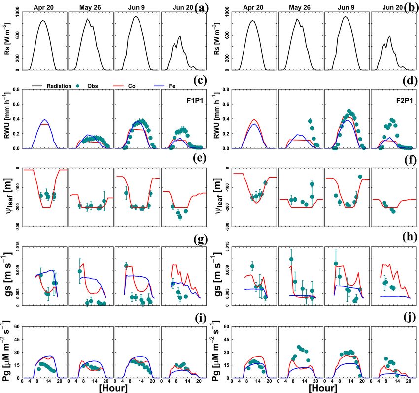
4946                     T. H. Nguyen et al.: Comparison of root water uptake models in simulating CO2 and H2 O fluxes

time records of photosynthetic active radiation, vapor pres-        plant organs (green leaf, brown leaf, stem, ear, and grain) and
sure deficit, and leaf temperature provided by the instru-          weighed. Subsamples were extracted afterward from these
ment. Then the leaves were quickly detached by a sharp knife        samples, weighed, dried in an oven at 105 ◦ C for 48 h, and
to measure leaf water pressure head with a digital pressure         weighed again for determining dry matter. At the end of the
chamber (SKPM 140/(40-50-80), Skye Instrument Ltd, UK).             growing season, four replicates of 1 m2 of plants were har-
   Plant hydraulic conductance in crop species can be esti-         vested from the plots to determine grain yield and harvest
mated by measuring the transpiration and the root zone and          index.
leaf water hydraulic heads (Tsuda and Tyree, 1997). In our
study, we calculated the conductance according to Ohm’s law         2.3     Model description
by dividing the hourly sap flow by the difference between
effective root zone hydraulic head and leaf hydraulic head.         2.3.1    Description of the original LINTULCC crop
The effective root zone hydraulic head was calculated based                  model
on hourly measured soil water hydraulic head and measured
                                                                    We used the crop model LINTULCC2 (Rodriguez et al.,
root length density (cm cm−2 ) at six depths (10, 20, 40, 60,
                                                                    2001). LINTULCC2 couples photosynthesis to stomatal con-
80, and 120 cm) in the soil profile following Eqs. (8) and (10)
                                                                    ductance and can perform a detailed calculation of leaf en-
(see Sect. 2.3.4). During one measurement day, six hourly
                                                                    ergy balances (Rodriguez et al., 2001; see Appendix A). This
values of the conductance were obtained from measurements
                                                                    model was validated and compared with different crop mod-
between 11:00 and 16:00 LT. The average and standard devi-
                                                                    els for spring wheat and used to simulate the effects of el-
ation of these hourly measurements were calculated for each
                                                                    evated CO2 and drought conditions (Ewert et al., 2002; Ro-
measurement day. However, the hydraulic conductance can
                                                                    driguez et al., 2001). LINTULCC2 calculates phenology, leaf
vary within short time periods due to the role of aquaporins
                                                                    growth, assimilate partitioning, and root growth following
(Maurel et al., 2008; Javot and Maurel, 2002; Henzler et al.,
                                                                    the procedure outlined in Rodriguez et al. (2001).
1999) or abscisic acid (ABA) regulation (Parent et al., 2009)
                                                                       In LINTULCC2, the assimilation rate of the sunlit and
and xylem cavitation (Sperry et al., 2003). We assumed how-
                                                                    shaded leaf is calculated using the biochemical model of
ever a constant plant hydraulic conductance during the day.
                                                                    Farquhar and von Caemmerer (1982). Stomatal conduc-
   Canopy gas exchange was measured hourly on the same
                                                                    tance (gs ) was calculated according to the model Leun-
days when leaf water pressure heads were measured with
                                                                    ing (1995) for sunlit and shaded leaves separately. In LIN-
a closed chamber system (Langensiepen et al., 2012). CO2
                                                                    TULCC2 CO2 uptake is calculated as a function of CO2 de-
concentration was derived with a regression approach by
                                                                    mand by photosynthesis and the ambient concentration of
Langensiepen et al. (2012). Because we were interested in
                                                                    CO2 , using the iterative methodology proposed by Leun-
comparing measured with calculated hourly instantaneous
                                                                    ing (1995) (Appendix A). For the sake of simplification, in
gross assimilation by the newly coupled root–shoot model
                                                                    LINTULCC2, the internal leaf CO2 concentration, Ci , is ini-
(LINTULCC2 with other subroutines), the total soil respira-
                                                                    tially assumed to be 0.7 times the atmospheric CO2 concen-
tion (i.e., heterotrophic organisms and root respiration) was
                                                                    tration Ca (Vico and Porporato, 2008; Rodriguez et al., 2001;
subtracted from the instantaneous canopy CO2 exchange rate
                                                                    Jones, 1992). Then, the light-saturated photosynthetic rate
measured by the closed chamber. The total soil respiration
                                                                    of sunlit and shaded leaves (AMAXsun and AMAXshade;
was calculated based on measured soil temperature, soil wa-
                                                                    µM CO2 m−2 s−1 ) and the quantum yield for sunlit and
ter content at 10 cm soil depth, and leaf area index from crops
                                                                    shaded leaves (EFFsun and EFFshade; µM CO2 MJ−1 ) are
using the fitted parameters derived from the same field and
                                                                    calculated iteratively (Farquhar et al., 1980; Farquhar and
soil types (Prolingheuer et al., 2010). The calculated total soil
                                                                    von Caemmerer, 1982). This iterative loop ends when the dif-
respiration was compared and validated with the measured
                                                                    ference in calculated internal CO2 mole fraction between two
values in the same field in the previous years from Stadler et
                                                                    consecutive loops is < 0.1 µmol mol−1 (Appendix A). Based
al. (2015).
                                                                    on a fraction of sunlit (and shaded) leaf area and leaf area
                                                                    index (LAI), the leaf stomatal resistance of sunlit and shaded
2.2.3   Crop growth
                                                                    leaves was integrated over the canopy leaf area to the canopy
                                                                    resistance (rs ) (Appendix B).
Crop growth information was collected biweekly from
                                                                       The canopy resistance, crop height, and calculated crop
20 April until harvest on 26 July 2016. Leaf area index and
                                                                    albedo (depending on both crop and soil water content of the
crop biomass were measured by harvests of two rows (1 m
                                                                    surface layer) and the surface energy balance were used to
each) for each treatment. Leaves were separated into green
                                                                    calculate potential crop evapotranspiration (ETP in mm h−1 )
leaves and brown leaves, and the brown and green leaf area
                                                                    using the Penman–Monteith equation (Allen et al., 1998; see
was measured using a leaf area meter (LI-3100C, Licor Bio-
                                                                    Appendix B). The obtained potential surface evapotranspira-
sciences, and Lincoln, Nebraska, USA). The aboveground
                                                                    tion is then split into evaporation and potential transpiration
biomass was measured using the oven drying method. Sam-
                                                                    using
ples were first weighed in total, then separated into different

Hydrol. Earth Syst. Sci., 24, 4943–4969, 2020                                        https://doi.org/10.5194/hess-24-4943-2020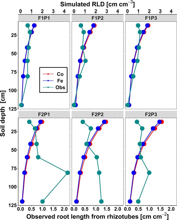
T. H. Nguyen et al.: Comparison of root water uptake models in simulating CO2 and H2 O fluxes                                    4947

                                                                      RSROOT depends on the soil temperature and is constrained

Tpot = ETP 1 − e    −kLAI
                                ,                              (1)    by a maximal elongation rate, RSROOTmax , and the soil-
                                                                      temperature-dependent rate, which is an empirical function
                                                                      of the soil temperature of the deepest layer where roots are
where k is the light extinction coefficient (0.6 in this study;
                                                                      growing, TBOTLAYER (K) (Jamieson and Ewert, 1999):
De Faria et al., 1994; Mo and Liu, 2001; Rodriguez et al.,
2001).                                                                RSROOT = min (RSROOTmax , TBOTLAYER · RTFAC),                (5)
   Tpot (mm h−1 ) represents by definition the transpiration of
the crop that is not limited by the root zone water hydraulic         where RTFAC is the temperature factor driving the penetra-
head. In Sect. 2.3.4 it is explained how the actual transpi-          tion of seminal roots (m K−1 d−1 ) and TBOTLAYER (K) the
ration, Tplant (mm h−1 ), is calculated as a function of the          soil temperature of the deepest layer where roots are grow-
potential transpiration and the root zone soil water pressure         ing. When soil temperature is below or equal to 0 ◦ C, no sem-
head. The ratio Tplant /Tpot defines the water stress factor fwat ,   inal growth occurs. The maximum daily elongation rate of
which is used in the photosynthesis model:                            seminal roots, RSROOTmax , was set at 0.03 m d−1 for wheat
                                                                      according to Watt et al. (2006).
         Tplant                                                          The daily increment in seminal root length (SRLIR;
fwat =          .                                              (2)
          Tpot                                                        m m−2 d−1 ) is defined as

Originally, LINTULCC2 runs at daily time steps (which al-             SRLIR = ASROOT/WSROOT.                                       (6)
lows for the within-day variations in temperature, radiation,
and vapor pressure deficit). LINTULCC2 requires daily max-            Lateral roots are simulated when the root biomass supplied
imum and minimum temperature, actual vapor pressure, rain-            by the shoot is greater than the assimilate demand of sem-
fall, wind speed, and global radiation. In order to capture           inal roots (RWRT > ASROOTdemand ). Lateral root biomass
the diurnal response of stomata, we modified the time step            is distributed stepwise from the top layer to the deepest soil
of the photosynthesis and stomatal conductance subroutine             layer with seminal roots.
from daily to hourly, while daily time steps were kept in the            Roots start to die after anthesis. Since the specific weight
remaining subroutines (phenology, leaf growth, and biomass            of the roots of cereal crops varies with soil strength (Colombi
partition).                                                           et al., 2017; Lipiec et al., 2016; Hernandez-Ramirez et al.,
                                                                      2014; Merotto and Mundstock, 1999), we chose different
2.3.2    Root growth model                                            specific weights for the stony (F1) and silty soil (F2) from the
                                                                      range that was observed by Noordwijk and Brouwer (1991)
Root growth was simulated using SLIMROOT (Addiscott                   and Jamieson and Ewert (1999) in soils with different soil
and Whitmore, 1991). The vertical extension of the semi-              strength (Appendix C).
nal roots and the distribution of the lateral roots within the
soil profile depend on the root biomass, the soil bulk density,       2.3.3   Physically based soil water balance model
the soil water content calculated by HILLFLOW 1D (Bron-
stert and Plate, 1997), and the soil temperature computed by          HILLFLOW 1D was chosen for calculating the water pres-
STMPsim (Williams and Izaurralde, 2005). The supply of                sure heads in the soil and how they change with depth and
assimilates from the shoot (RWRT; g m−2 d−1 ) is given by             time as a function of the precipitation, soil evaporation,
a partitioning table based on the thermal time (van Laar et           RWU, and water percolation at the bottom of the simulated
al., 1997) that is used to calculate the vertical penetration of      soil profile (Bronstert and Plate, 1997). HILLFLOW 1D cal-
seminal and lateral roots. The assimilate allocation for sem-         culates soil water content and water fluxes by numerically
inal root growth (ASROOT) is constrained by daily supply              solving the Darcy equation for unsaturated water flow in
of assimilates from the shoot RWRT (g m−2 d−1 ) and the de-           porous media (Bronstert and Plate, 1997). The relations be-
mand of assimilates from seminal roots (ASROOTdemand ).               tween soil water hydraulic head, water content, and hydraulic
                                                                      conductivity are described by the Mualem–van Genuchten
ASROOT = min (ASROOTdemand , RWRT)                             (3)    functions (van Genuchten, 1980). The parameters of these
                                                                      functions, i.e., the soil hydraulic parameters, for the different
ASROOTdemand is a function of the number of seminal roots             soil layers and the two sites were taken from Cai et al. (2018)
per square meter (NSROOT), which depends on the num-                  (Appendix D). In this study, a soil depth of 1.5 m vertically
ber of emerged plants per square meter and the number of              discretized into 50 layers was considered. A free drainage
seminal roots per plant, the specific weight of seminal roots         bottom boundary and a mixed flux-matric potential bound-
WSROOT (g m−1 ), and the daily elongation rate of seminal             ary at the soil surface were implemented. The mixed upper
roots RSROOT (m d−1 ):                                                boundary condition prescribes the flux at the soil surface by
                                                                      the precipitation and evaporation rates as long as the soil
ASROOTdemand = RSROOT · WSROOT · NSROOT.                       (4)    water pressure heads are not above or below critical heads.

https://doi.org/10.5194/hess-24-4943-2020                                          Hydrol. Earth Syst. Sci., 24, 4943–4969, 2020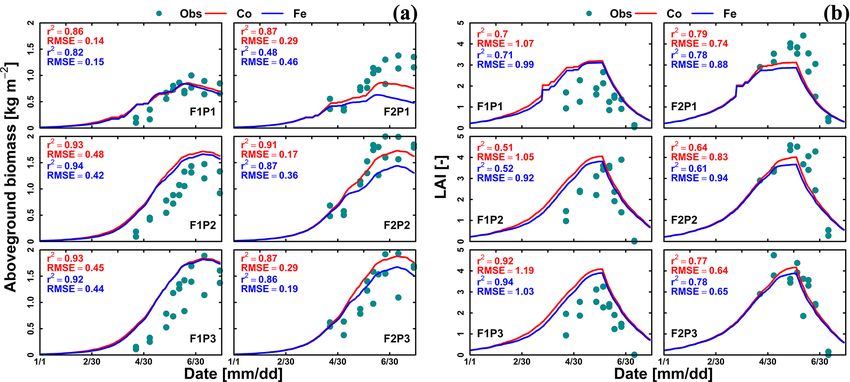
4948                         T. H. Nguyen et al.: Comparison of root water uptake models in simulating CO2 and H2 O fluxes

When these heads are reached, the boundary conditions are          draulic head is calculated as the weighted average of the hy-
switched to constant pressure head boundary conditions.            draulic heads in the different soil layers as
                                                                           N
2.3.4   Feddes’ and Couvreur’s root water uptake
                                                                           X
                                                                   ψsr =         ψi NRLDi 1zi .                                (10)
        models                                                             i=1

The Feddes RWU model (Feddes et al., 1978; see Ap-                 The plant transpiration rate is the minimum of the
pendix E) was already built in the HILLFLOW 1D model               potential transpiration rate and the transpiration rate,
(Bronstert and Plate, 1997). We implemented the Couvreur           Tthreshold (mm h−1 ), when the hydraulic head in the leaves
RWU model (Couvreur et al., 2012, 2014) into HILLFLOW.             reaches a threshold value, ψthreshold (m), that triggers stom-
In both models, Tplant is calculated from the sum of the sim-      atal closure:

ulated RWU in the different soil layers and used to calculate      Tplant = max 0, min Tpot , Tthreshold .                    (11)
the water stress factor (fwat ) following Eq. (2), which was
used in the photosynthesis model. In the Feddes model, root        Tthreshold is calculated from the difference between the root
water uptake from a soil layer is proportional to the normal-      zone hydraulic head and the threshold hydraulic head in the
ized root density, NRLD (m−1 ), in that layer and is multi-        leaves ψthreshold that is multiplied by the plant hydraulic con-
plied by a stress function α that depends on the soil water        ductance, Kplant as

pressure head, ψm (m), in that soil layer and the potential        Tthreshold = Kplant ψsr − ψthreshold .                      (12)
transpiration rate (see Appendix E for the definition of α):
                                                                   In our study, we used the critical leaf hydraulic head,

RWUi = α ψm,i , Tpot Tpot NRLDi 1zi ,                       (7)    ψthreshold , of −200 m (equivalent to −2 MPa) (Cochard,
                                                                   2002; Tardieu and Simonneau, 1998). The original Couvreur
where NRLDi is calculated from the root length density,            model only considers the hydraulic conductance from the
RLD (m m−3 ), and discretized soil dept, 1zi (m), as               roots to the plant collar, Krs , by assuming that the hydraulic
                                                                   resistance from plant collar to leaves is minor as compared to
                   N
                   X                                               root system resistance. The shoot hydraulic resistance could
NRLDi = RLDi /           RLDi 1zi .                         (8)    be large in some crop plants (Gallardo et al., 1996) or in trees
                   i=1                                             (Domec and Pruyn, 2008; Tsuda and Tyree, 1997). In order
                                                                   to simulate the leaf water hydraulic head, the whole plant
The parameters of the α stress functions model were taken          hydraulic conductance (Kplant ) needs to be used. The whole
from Cai et al. (2018; see Appendix C). According to Eq. (7),      plant hydraulic conductance could be estimated from differ-
the reduction of water uptake in a given layer depends on the      ent components (i.e., soil to roots, stem to leaf) following an
soil water pressure head in that layer only and does not in-       approach from Saliendra et al. (1995) or a more complex at-
fluence the water uptake in other layers. This means that a        tempt by Janott et al. (2011). Because hydraulic data from
reduced water uptake in dried out soil layers directly leads to    plant collar to leaf are rare and difficult to obtain and account
a reduction of the total root water uptake and plant transpi-      for differing species characteristics and environmental condi-
ration and is not compensated by increased uptake in other         tions, for the sake of simplification, we derived Kplant (d−1 )
layers where there is still water available.                       from the root hydraulic conductance (Krs ,doy ), assuming that
   In the Couvreur model, the root water uptake in a given         Kplant is a constant fraction β of Krs ,doy (d−1 ):
soil layer is related to the water potentials in the root system
and root water uptake in other soil layers so that compen-         Kplant = β Krs ,doy .                                       (13)
satory uptake is considered in this model. Root water uptake       We used the measured plant hydraulic conductance from sap
in a certain layer is obtained from                                flow, leaf water hydraulic head, soil water pressure head,
                                                                  and root observation (Sect. 2.2.1 above) in the lower rain-
RWUi = Tplant NRLDi 1zi + Kcomp ψi − ψsr NRLDi 1zi , (9)           fed plot to calibrate β, which was then applied for all plots
                                                                   (Appendix C). Kplant and Krs in anisohydric wheat are influ-
where ψi (m) is the total hydraulic head (or hydraulic head        enced by soil water availability and crop development. We
which is the sum of the pressure head and gravitation poten-       followed the approach of Cai et al. (2017) to estimate the
tial heads) in layer i, ψsr (m) is the average hydraulic head      root hydraulic conductance (Krs ,doy ) and compensatory root
in the root zone, and Kcomp (d−1 ) is the root system con-         water uptake (Kcomp ) based on the total length of the root
ductance for compensatory uptake. The first term of Eq. (9)        system below a unit surface area, TRLDdoy (m m−2 ), at a
represents the uptake from that soil layer when the hydraulic      given day of year (DOY) (Eq. 14), which is the output from
head is uniform in the root zone, and the second term rep-         SLIMROOT:
resents the increase or decrease of uptake from the soil layer                     N
due to a respectively higher and lower hydraulic head in layer
                                                                                   X
                                                                   TRLDdoy =            RLDi,doy 1zi .                         (14)
i than the average hydraulic head. The average root zone hy-                        i

Hydrol. Earth Syst. Sci., 24, 4943–4969, 2020                                           https://doi.org/10.5194/hess-24-4943-2020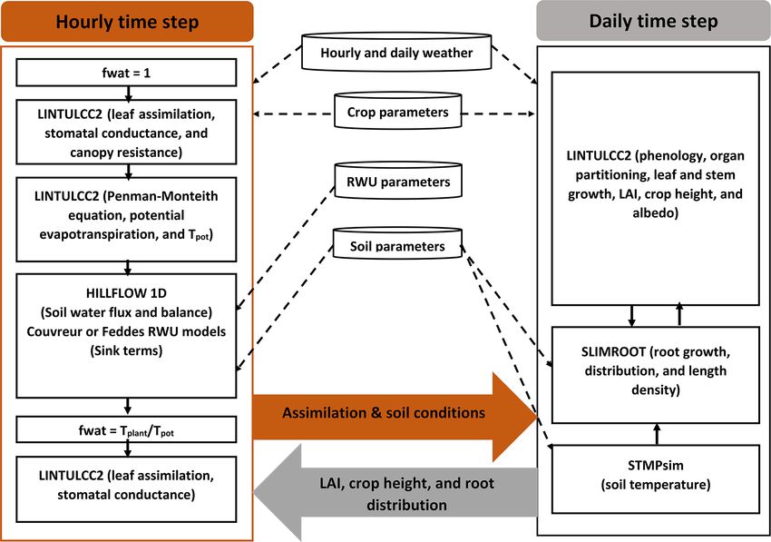
T. H. Nguyen et al.: Comparison of root water uptake models in simulating CO2 and H2 O fluxes 4949
Assuming the same conductance for all root segments, the ◦ C d) were used for phenology calibration based on infor-
root system conductance scales with the TRLD: mation of sowing, anthesis, and maturity dates. The model
was then calibrated using time series of LAI, biomass, and
Krs ,doy = Krs ,normalized TRLDdoy , (15) gross assimilation rate through the change of maximum car-
boxylation rate at 25 ◦ C (VCMAX25), critical leaf area in-
where Krs ,normalized (d−1 cm−1 cm2 ) is the root sys-
dex (LAICR), and relative growth rate of leaf area during ex-
tem conductance per unit root length per surface area.
ponential growth (RGRL) parameters. The same crop param-
For Krs ,normalized , we took the average value that was ob-
eters and soil parameters were applied for both model config-
tained by Cai et al. (2018) for the stony soil (F1) and silty
urations (Appendices C and D). All presented flux data (soil
soil (F2) sites: 0.2544 × 10⁻⁵ (cm d−1 ) (Appendix C).
water flux, gross assimilation rate, sap flow, stomatal con-
Many studies included hydraulic conductance along the
ductance, and leaf water pressure head) and the simulated
soil–plant–atmosphere pathway to simulate water transport
outputs were converted from local time to coordinated uni-
(Verhoef and Egea, 2014; Wang et al., 2007; Tuzet et al.,
versal time (UTC) to avoid the confusion in interpretation.
2003; Olioso et al., 1996). However, both root and plant hy-
draulic conductance in these studies were assumed constant. 2.4 Criteria for model comparison and evaluation
In our work, the plant hydraulic conductance varied follow-
ing the shoot and root development in the growing season. We analyzed the performance of two modeling approaches
following the approach from Willmott (1981): (i) correla-
2.3.5 Coupling of water balance and root water uptake tion coefficient (r) (Eq. 16); (ii) the degree to which simu-
models with the crop model lated values approached the observations or index of agree-
ment (I ) defined in Eq. (17), varying from 1 (for perfect
We carried out a comprehensive comparison of the following
agreement) to 0 (for no agreement); (iii) the root mean square
modeling approaches for simulating CO2 and H2 O fluxes and
error (RMSE), computed to characterize the difference be-
crop growth (Fig. 2):
tween simulated values and observed data (Eq. 18):
– HILLFLOW 1D–Couvreur’s RWU–SLIMROOT– n
P
LINTULCC2 (Co) Simi − Sim Obsi − Obs
i=1
– HILLFLOW 1D–Feddes’ RWU–SLIMROOT– r = s (16)
n n
P 2 P 2
LINTULCC2 (Fe). Simi − Sim Obsi − Obs
i=1 i=1
The photosynthesis and stomatal conductance subroutines, n
(Simi − Obsi )2
P
RWU and HILLFLOW 1D water balance model, and evap-
orative demand (ETP) were run or specified with hourly
i=1
I = 1− n
(17)
time steps, while phenology, leaf growth, root growth, and
P 2
Simi − Obs + |Obsi − Obs|
biomass partitioning were updated daily. For a certain hourly i=1
time step 1ti = ti − ti−1 , different modules were solved in v
u n
uP
the following sequence. First, LINTULCC2 was used with a u (Simi − Obsi )2
water stress factor fwat = 1 to calculate the leaf and canopy
t i=1
RMSE = , (18)
resistance and the potential transpiration rate. Tpot was then n
used in HILLFLOW 1D to calculate the soil water pressure where Sim and Obs are simulated and measured variables;
head changes, water content changes, the actual transpira- i is the index of a given variable; Obs and Sim are the mean
tion, and fwat during the time step. LINTULCC2 was then of the simulated and measured data; and n is the number of
run again using fwat . The leaf conductance and assimila- observations.
tion rate were calculated. For the next time step, the same
loop was run, and hourly assimilation was accumulated to 2.5 Sensitivity analysis
a daily value. Daily assimilation rates were used in mod-
ules that run with a daily time step, for instance, modules The parameters of the SLIMROOT root growth model and
of LINTLCC2 that calculate assimilate partitioning which the Couvreur RWU model were derived from literature data.
is used to calculate shoot (LAI) development and passed However, these parameters are uncertain and vary between
to SLIMROOT to simulate root development (Fig. 2). Be- different wheat varieties. In order to evaluate the effect of
fore comparing these modeling approaches, we calibrated these parameters on the simulated crop growth and root water
the original LINTULCC model using the data from the rain- uptake, we carried out a sensitivity analysis.
fed plots in the silty soil (F2P2). The model is firstly cali- In a first set of simulations, the root length normalized
brated to make sure the model properly described the phe- root system conductivity Krs ,normalized was varied from 0.1 to
nology. Two parameters (minimum thermal sum from sow- 40 times the Krs ,normalized = 0.2554 × 10⁻⁵ cm d−1 that was
ing to anthesis and thermal sum from anthesis to maturity; estimated by Cai et al. (2018). The root system hydraulic
https://doi.org/10.5194/hess-24-4943-2020 Hydrol. Earth Syst. Sci., 24, 4943–4969, 2020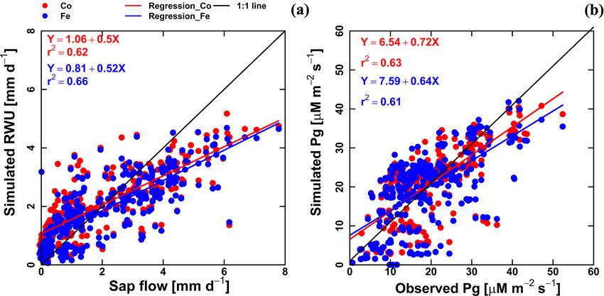
4950                      T. H. Nguyen et al.: Comparison of root water uptake models in simulating CO2 and H2 O fluxes

Figure 2. Description of the coupled root–shoot models in the study. The orange arrow indicates feedbacks from the hourly simulations to
daily simulation, while the grey arrow indicates feedbacks from the daily simulations to the hourly simulations. The dashed black arrows
denote the weather input and parameters to the subroutines. The continuous black arrows indicate the links amongst the modeling subroutines.

conductance is related to the total root length, which depends          (Co model) and Feddes RWU model (Fe model). The com-
on the specific weight of lateral and seminal roots. These              parative analysis firstly focuses on simulating crop growth
two parameters are rarely reported, especially for field-grown          and root development under different water conditions and
wheat (Noordwijk and Brouwer, 1991). The observed spe-                  soil types. Next, the simulated transpiration reduction, soil
cific weight of lateral roots in wheat was reported to be in the        water dynamics, RWU, and gross assimilation rate are pre-
range of 0.00406 to 0.00613 g m−1 (Noordwijk and Brouwer,               sented and discussed. The Kplant is explicitly simulated by
1991). Huang et al. (1991) found that the specific weight of            the Co model in the different soils and treatments and is
seminal roots of winter wheat grown under controlled soil               compared with direct estimates of Kplant from measure-
chamber conditions decreased from 0.023 to 0.0052 g m−1                 ments. In the second part, we discuss the sensitivity anal-
when air temperature increased from 10 to 30 ◦ C. The values            ysis of the Co model to understand the effects of chang-
of 0.015 and 0.0035 g m−1 are often used for specific weights           ing Krs ,normalized , the specific weight of seminal and lateral
of seminal and lateral roots, respectively, in crop growth              roots, and 9threshold on the simulated biomass growth and
simulations of wheat cultivars (Mboh et al., 2019; Jamieson             RWU in different soils and under different water regimes.
and Ewert, 1999). In a second set of simulations, the spe-
cific weight of lateral roots was changed from 0.002, 0.003,            3.1     Comparison of Couvreur’s and Feddes’ RWU
0.0035, 0.004, 0.005, 0.006, and 0.007 g m−1 , while the spe-                   model
cific weight of seminal roots was the same (0.015 g m−1 )
for all simulations. For the third set of simulations, the              3.1.1    Root and shoot (biomass and LAI) growth
specific weight of lateral roots was kept at 0.0035 g m−1 ,
while the specific weight of seminal roots varied from 0.005,           Figure 3 shows the dry matter and LAI simulated by the
0.0075, 0.01, 0.0125, 0.015, 0.0175, 0.02, and 0.0225 g m−1 .           Co and Fe model versus the measured data. The difference
In the last sensitivity exercise, the critical leaf hydraulic head      between the two samples of the two different rows for each
threshold (ψthreshold ) was varied between −120 and −260 m.             sampling day indicated the heterogeneity in crop growth,
                                                                        even within a small treatment plot. Biomass and LAI sim-
                                                                        ulated by the Co and Fe models were in fair agreement
3   Results and discussion                                              with observations. The r 2 values of the Co and Fe models
                                                                        were 0.91 and 0.86, respectively, for biomass, while they
In the first section, we discuss the performance of the two             were 0.76 and 0.75, respectively, for LAI (Table 1). How-
coupled root–shoot models with the Couvreur RWU model                   ever, both models overestimated dry matter and LAI produc-

Hydrol. Earth Syst. Sci., 24, 4943–4969, 2020                                             https://doi.org/10.5194/hess-24-4943-2020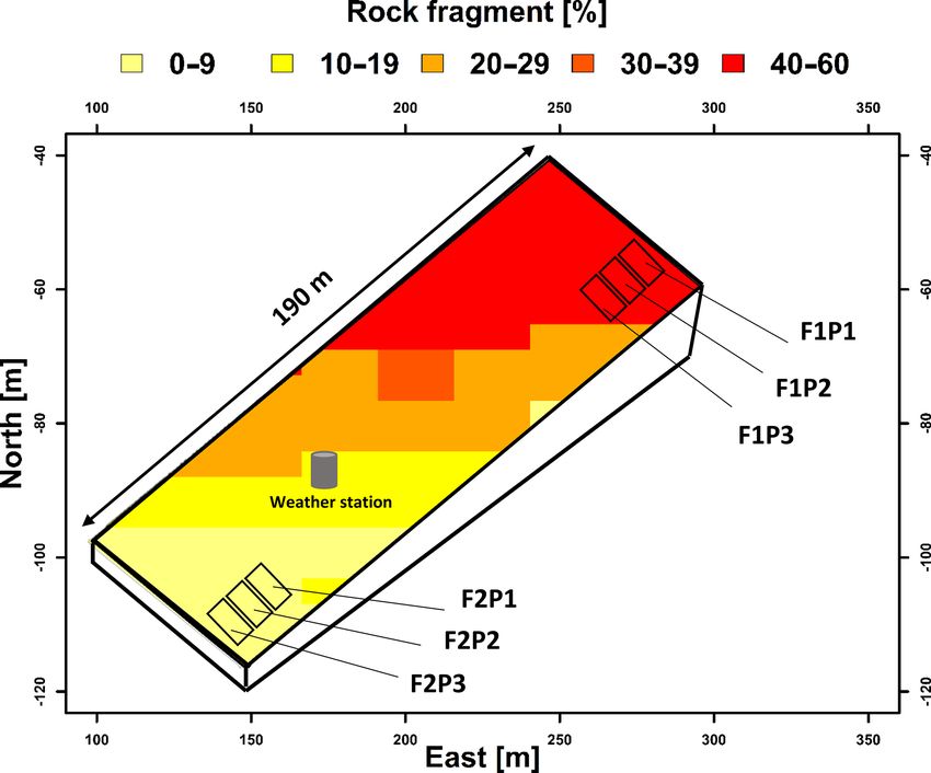
T. H. Nguyen et al.: Comparison of root water uptake models in simulating CO2 and H2 O fluxes                                                 4951

Figure 3. Comparison between observed (cyan dot) and simulated (a) aboveground dry matter and (b) LAI by Couvreur (Co; solid red line)
and Feddes (Fe; solid blue line) model in the sheltered (P1), rainfed (P2), and irrigated (P3) plots of the stony soil (F1) and the silty soil (F2).
Note that crop germination was on 26 October 2015; data are shown here from 1 January to harvest on 23 July 2016. RMSE in (a) is kg m−2
while RMSE in (b) is unitless.

tion in the irrigated and rainfed stony plots, whereas biomass
and LAI were underestimated in the sheltered silty plot. This
suggests that water stress in the sheltered silty plot was over-            Table 1. Quantitative and statistical measures of the comparison
estimated. For the irrigated stony soil plot, in which the wa-              between two modeling approaches and the observed data for the
ter content stayed high due to the frequent rainfall events and             three water treatments and two soil types. RMSE is the root mean
the additional irrigation, it is unlikely that the lower growth             square error; r 2 is the correlation coefficient; I is the agreement in-
                                                                            dex; n samples is the number of samples. Co is the Couvreur RWU
is due to water stress. The later start of the growth after the
                                                                            model, and Fe is the Feddes RWU model.
winter could be due to the effects of soil strength and lower
soil temperature on crop development in the stony field that
                                                                                         Variables          Statistical     Co      Fe
were not captured by the model. Soil hardness could con-                                                    indexes
strain root growth while the higher stone content possibly
resulted in slower warming up of the soil in spring than the                             Daily RWU          RMSE          1.15    1.13
silty soil which in turn slowed down root and crop develop-                              (mm d−1 )          r2            0.62    0.66
ment.                                                                                                       I             0.84    0.85
                                                                                                            n samples     312      312
   For the stony plots, the Fe and Co models gave similar
results, whereas for the silty soil, the Co model reproduced                             Biomass            RMSE           303     336
the biomass and LAI better than the Fe model. Although the                               (g m−2 )           r2            0.91    0.86
statistical parameters (r 2 and RMSE) for the silty soil plots                                              I             0.84    0.81
show only a slightly better fit of the Co than of the Fe model,                                             n samples       54      54
there is a remarkable qualitative difference between the mod-                            LAI                RMSE          0.92    0.90
els. The Fe model simulated lower biomass and leaf area in                               (–)                r2            0.76    0.75
the silty soil than in the stony soil, which is opposite to the                                             I             0.77    0.77
observations. The Co model simulated similar biomass and                                                    n samples       54      54
LAI in the irrigated and rainfed plots of the silty and stony
                                                                                         Gross              RMSE          6.34    7.26
soils and higher biomass and LAI in the sheltered plot in silty
                                                                                         assimilation       r2            0.63    0.61
soil than in the stony soil, which is in closer agreement with                           rate               I             0.86    0.83
the observed differences in biomass and LAI between the two                              (µM m−2 s−1 )      n samples     302      302
soils. The simulated effect of the soil type on the crop growth

https://doi.org/10.5194/hess-24-4943-2020                                                  Hydrol. Earth Syst. Sci., 24, 4943–4969, 2020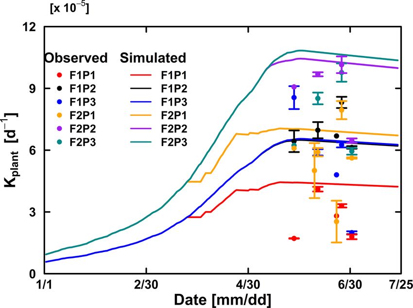
4952 T. H. Nguyen et al.: Comparison of root water uptake models in simulating CO2 and H2 O fluxes
plot to the reference were for all plots larger than 1. Never-
theless, the ratios of observed root lengths were larger (2.27–
4.03) than those of the simulated ones (1.04–1.67). The ob-
served ratios were larger for the sheltered plot than for the
other plots in the silty soil, whereas the opposite was sim-
ulated by the models. Predefined ratios of root and shoot
biomass allocation for a given growth period and a source-
driven root growth (van Laar et al., 1997) in our models do
not allow a shift in carbon allocation to roots (for more root
growth) in response to water stress. However, this should not
be emphasized too much because the observed imaged root
data from minirhizotubes for driving the root length might
have potential errors and uncertainties (Cai et al., 2018).
3.1.2 Transpiration reduction, soil water dynamic,
RWU, and gross assimilation rate
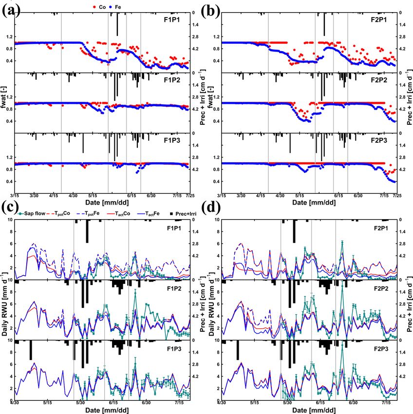
Figure 5a and b show the reduction of the transpiration com-
pared to the potential transpiration, fwat , simulated by the
Fe and Co models (mid-March until harvest), and Fig. 5c
and d show the simulated potential and the simulated and
measured actual transpiration rates from the end of April un-
Figure 4. Comparison between observed root length from rhizo- til harvest. The Fe model simulated more water stress than
tubes (cm cm−2 ) (cyan line with dots) and simulated root length
the Co model and a more pronounced and earlier stress in
density (RLD) (cm cm−3 ) from 10, 20, 40, 60, 80, and 120 cm
soil depth at DOY 149 by the Couvreur (Co; solid red) and Fed-
the silty than in the stony soil. As a consequence, the sim-
des (Fe; solid blue) model in the sheltered (P1), rainfed (P2), and ulated transpiration rates by the Fe model were generally
irrigated (P3) plots of the stony soil (F1) and the silty soil (F2). lower than the simulated ones by the Co model. According
to the fwat factors, the Couvreur model also simulated more
water stress in the silty soil than in the stony soil. The ef-
fect of fwat on the cumulative transpiration and growth also
was qualitatively correct for the Co model but incorrect for depends on the timing of the lower fwat values. At the be-
the Fe model. ginning of the growing season when the LAI and potential
Figure 4 displays the observed root length densities from transpiration are low, the impact of a lower fwat on the cu-
minirhizotube observations and the simulated ones. Higher mulative transpiration and growth is lower than later in the
root length densities were observed and simulated in the silty growing season. These results are in contrast with findings
soil than in the stony soil. The model simulated smaller root by Cai et al. (2017, 2018), who found that there was no wa-
densities in the stony soil because a larger specific weight of ter stress simulated in the silty soil in 2014 by the Co and
the roots was considered for the stony soil than for the silty Fe models. However, the studies from Cai et al. (2018) used
soil. The simulated root density profiles showed the highest the measured root distributions instead of the simulated ones
root densities near the surface, whereas the observed profiles, from the root–shoot model. Therefore, in their simulations,
especially in the silty soil, showed higher densities in the the crop had more access to water in the deeper soil layers.
deeper soil layers. The model simulated smaller root length Second, they used the Feddes–Jarvis model, which accounts
densities in the sheltered plots than in the other plots of both for root water uptake compensation. This could explain why
the stony and silty soils. This is a consequence of the lower they did not simulate water stress in the silty plot with the
biomass growth that was simulated in the sheltered plots. For Feddes model. Thirdly, weather conditions and irrigation ap-
the stony soil, this corresponds with the observations that plications were different in their study in 2014 (less dry) from
also showed lower root length densities in the sheltered plots our experimental season in 2016.
than in the other plots. However, for the silty plot, the oppo- According to Fig. 5c and d, during the time when sap flow
site was observed. For both the simulations and the observa- could be measured (from end of May until harvest), the stress
tions, we compared the ratio of total root lengths in a certain factors did not differ a lot between the Fe and Co models. For
plot and treatment to the total root length in the rainfed stony the rainfed and irrigated plots in the silty soil, the Fe model
plot F1P2 (Appendix F). In the stony plots the ratios of the predicted a stronger reduction in transpiration near the end
observed total root length to the reference were close to 1, of the growing season than the Co model. This resulted in a
but the simulated total root length in the sheltered plot was smaller cumulative transpiration predicted by the Fe model
smaller than 1. The ratios of the total root lengths in the silty than by the Co model over the measurement period in these
Hydrol. Earth Syst. Sci., 24, 4943–4969, 2020 https://doi.org/10.5194/hess-24-4943-2020T. H. Nguyen et al.: Comparison of root water uptake models in simulating CO2 and H2 O fluxes 4953 Figure 5. Daily transpiration reduction factor (fwat ) (a, b) from 15 March to harvest on 23 July 2016 and comparison between observed (cyan) and simulated root water uptake (RWU) and potential transpiration simulated (c, d) by the Couvreur (Co; closed red) and Feddes (Fe; closed blue) models from 30 April to 20 July 2016 in the sheltered (P1), rainfed (P2), and irrigated (P3) plots of the stony soil (F1) and the silty soil (F2). Time series of precipitation (Prec) and irrigation (Irri) are given in the panels. Note that crop germination was on 26 October 2015. Vertical cyan bars represent the standard deviation of the flux measurements in the different stems. Vertical grey lines show days with the measured and simulated diurnal courses of root water uptake (RWU), leaf water pressure head (ψleaf ), stomatal conductance (gs ), and gross assimilation rate (Pg ) as used in Fig. 9. https://doi.org/10.5194/hess-24-4943-2020 Hydrol. Earth Syst. Sci., 24, 4943–4969, 2020
4954                       T. H. Nguyen et al.: Comparison of root water uptake models in simulating CO2 and H2 O fluxes

Figure 6. Cumulative precipitation and irrigation (Prec + Irri), potential evapotranspiration (ETP), potential transpiration (Tpot ), and actual
transpiration (Tact or RWU) simulated by the Couvreur (Co) and Feddes (Fe) models and measured transpiration by sap flow sensors (Obs)
from 26 May to 20 July 2016 in the sheltered (P1), rainfed (P2), and irrigated (P3) plots of the stony soil (F1) and the silty soil (F2).

Figure 7. Correlation between observed and simulated (a) daily actual transpiration (or RWU), (b) hourly gross assimilation rate (Pg ) from
the Couvreur (Co; red dot) and Feddes (Fe; blue dot) models of both fields (F1 and F2). Sap flow data were from 26 May until 20 July 2017
(n = 312). Gross assimilation rate from 8 measurement days (n = 302). The RMSE in (a) is given in mm d−1 , while the RMSE in (b) is
given in µM m−2 s−1 .

treatments (Fig. 6). Although this gives the impression that              erage, the two models slightly underestimated measured Tact
the Co model is better in agreement with the measurements                 (Fig. 5c and d). This was also found in the study by Cai et
in these treatments, Fig. 5d indicates that this is due to com-           al. (2018), in which sap flow was measured in winter wheat
pensating errors. Both models underestimate the measured                  in 2014. However, in their study, there was a rather con-
sap flow in the beginning of the measurement period and                   stant offset between the simulations and the sap flow data.
overestimate it towards the end, and the Co model overes-                 One reason could be that in our study we used the simu-
timates more than the Fe model. This overestimation is due                lated LAI values, whereas Cai et al. (2018) used the mea-
to an overestimation of the LAI by both models near the end               sured LAI values. In the stony plots, the measured LAIs are
of the growing season (Fig. 3b). The reduction of the tran-               overestimated by the simulations so that one would expect
spiration in the sheltered plots of the two soils compared                an overestimation of the transpiration by the model. The op-
to the other treatments is predicted relatively well, but the             posite holds true for the silty plot. The overestimation of the
Fe model predicted more stress and a stronger reduction in                LAI at the end of growing season resulted in an overesti-
transpiration than the Co model, especially in the silty soil.            mation of the transpiration in nonsheltered plots in both soil
For this treatment, the Co model, which simulated less stress             types. Because of the small size and hollow stem of wheat
(larger fwat factors), predicted the cumulative transpiration             plants (Langensiepen et al., 2014), it is difficult to install the
and how it differed between the two soil types better than the            microsensors and measure the temperature variation for the
Fe model.                                                                 thin wheat stem with high time frequency under ambient field
   Simulated transpiration in all treatments and both soils are           conditions. In addition, the sap flow in a single tiller is also
plotted versus the sap flow measurements in Fig. 7. On av-                influenced by spatial variation in environmental conditions.

Hydrol. Earth Syst. Sci., 24, 4943–4969, 2020                                                https://doi.org/10.5194/hess-24-4943-2020
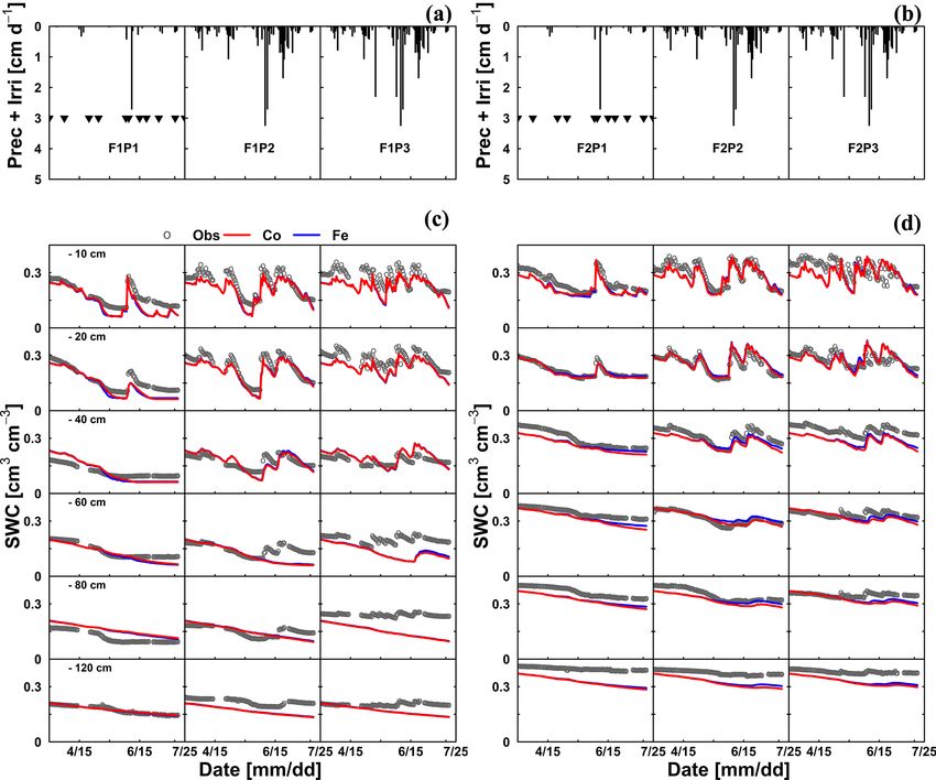
T. H. Nguyen et al.: Comparison of root water uptake models in simulating CO2 and H2 O fluxes                                  4955

The variability of stem development also results in a signif-       derborght et al., 2010). In our simulation, the use of a soil
icant stem-to-stem variability in sap flow (Cai et al., 2018).      depth of 1.5 m may not be deep enough to capture this ef-
The r 2 values of simulated RWU from the Co and Fe models           fect. The simulated SWC values were however very similar
versus sap flow are 0.62 and 0.66, respectively (Table 1 and        for both models. The larger RWU simulated by the Co than
Fig. 7a), indicating that our coupled models show a fair per-       by the Fe model in the silty soil in May resulted in slightly
formance in the RWU simulation. Measuring gas exchange              lower simulated water contents by the Co model. But, the dif-
with closed chamber concentration measurements can sig-             ferences in simulated water contents by the two models were
nificantly alter the microclimatic conditions within the cham-      much smaller than the deviations from the observed water
ber, especially at times of high exchange rate. However using       contents.
regression functions at the starting point of measurement in-          For a few selected days, the diurnal course of Tact
tervals reduces absolute errors (Langensiepen et al., 2012).        (or RWU), gross assimilation rate (Pg ), stomatal conduc-
The simulated gross assimilation rate (Pg ) from two mod-           tance (gs ), and leaf pressure head was measured. The mea-
els matched relatively well with the gross assimilation rate        sured and simulated data are shown in Fig. 9. Both Co and
measured by a manually closed-canopy chamber, with an               Fe models could mimic the daytime fluctuation of RWU and
r 2 value of 0.63 and 0.61 for Co and Fe, respectively (Ta-         Pg in the sheltered plot of the stony soil, which is consis-
ble 1 and Fig. 7b).                                                 tent with the adequate simulation of root growth (Fig. 4,
   The method that we used for modeling the canopy resis-           F1P1) and SWC dynamics (Fig. 8c, F1P1). When the simu-
tance used in the Penman–Monteith equation has been re-             lated ψleaf reached ψthreshold = −200 m, the simulated RWU
ported for both short and tall crops (Dickinson et al., 1991;       and Pg by the Co model showed a plateau (26 May in
Kelliher et al., 1995; Irmak and Mutiibwa, 2010; Perez et           Fig. 9c, e, and i). The Co model simulated the diurnal courses
al., 2006; Katerji et al., 2011; Srivastava et al., 2018). The      of stomatal conductance better as compared to the Fe model,
fair agreement of RWU to sap flow in our study indicates            especially on a day with water stress (26 May; Fig. 9g and h).
the proper estimate of ETP based on the crop canopy resis-          Using the leaf water pressure head threshold as an indication
tance (with fwat = 1) in winter wheat. The direct calculation       of water stress effects on stomata, Tuzet et al. (2003) and
of crop canopy resistance in our work allows physiological          Olioso et al. (1996) also reported a considerable drop of Pg
responses of the crop (stomatal conductance) to solar radi-         and transpiration. The sharp drop of simulated RWU and Pg ,
ation, temperature, and vapor pressure deficit (Eq. A5) to          which is in contrast with measurement on the same day in the
be captured. In addition, this approach also avoids calculat-       sheltered plot in silty soil, illustrated that both models over-
ing grass reference evapotranspiration based on a constant          estimated the water stress. This is related to the underestima-
canopy resistance.                                                  tion of both root growth (Fig. 4, F2P1) and SWC (Fig. 8d,
   The differences in simulated stress between the different        F2P1) in the deeper soil layers by two models.
models were more pronounced in May (Fig. 5) when no sap
flow data were available. The Co model predicted less stress        3.1.3   Whole plant hydraulic conductance from the
and more RWU than the Fe model in May, especially in the                    Couvreur RWU model
rainfed and irrigated plots of the silty soil. The larger stress
simulated by the Fe model in the rainfed and irrigated silty        The Couvreur RWU model considers the root hydraulic con-
plots resulted in a smaller increase in biomass that was simu-      ductance, which relies on absolute root length. The root
lated in May by the Fe model than by the Co model (Fig. 3a).        hydraulic conductance is used to upscale to whole plant
The measurements of growth in the silty soil do not suggest         hydraulic conductance. The simulated Kplants reproduced
that there was water stress in these plots in the silty soil, in-   the measured ones in the different treatments quite well
dicating that the Co model better simulated transpiration and       (Fig. 10). Our measured Kplant ranged from 1.5 × 10⁻⁵ to
growth for these cases than the Fe model. Another way to test       10.2×10⁻⁵ d−1 (Fig. 10). These values are on the same order
the RWU simulated by the different models is to compare the         of magnitude as values reported by Feddes and Raats (2004)
simulated soil water contents (Fig. 8). The Co and Fe models        for ryegrass ranging from 6 × 10⁻⁵ to 20 × 10−5 d−1 . The
were able to simulate both dynamics and magnitude of soil           simulated Kplant from our coupled root and shoot Co model
water content (SWC) in different soil depths and for different      followed the root growth and reached a maximum at around
water treatments (average of RMSEs over all soil depths was         anthesis. Kplant reduces toward the end of the growing sea-
0.06 for both models; Appendix G). The Co and Fe models             son due to root death. For the sheltered plot of the silty field,
displayed lower water contents than the measured ones in the        we would expect, based on the root density measurements
deeper layers at the late growing season (i.e., depth 80 and        (Fig. 4), the highest Kplant of all treatments. However, this
120 cm) (Fig. 8). This could be due to the free drainage bot-       was not observed in the field. Based on the measured total
tom boundary condition in the HILLFLOW water balance                root lengths, we would also expect that Kplant of the shel-
model, which implies that the water can only leave the soil         tered plot in the stony soil should be similar to Kplant in the
profile, but no water can flow into it from below. Capillary        other plots of the stony soil. But, Kplant was clearly lower in
rise in the soil can keep the lower layers relatively wet (Van-     the sheltered plot of the stony soil than in the other treatments

https://doi.org/10.5194/hess-24-4943-2020                                        Hydrol. Earth Syst. Sci., 24, 4943–4969, 2020
You can also read