Plant hydraulic transport controls transpiration sensitivity to soil water stress
←
→
Page content transcription
If your browser does not render page correctly, please read the page content below
Hydrol. Earth Syst. Sci., 25, 4259–4274, 2021
https://doi.org/10.5194/hess-25-4259-2021
© Author(s) 2021. This work is distributed under
the Creative Commons Attribution 4.0 License.

Plant hydraulic transport controls transpiration
sensitivity to soil water stress
Brandon P. Sloan1,2 , Sally E. Thompson3 , and Xue Feng1,2
1 Department of Civil, Environmental, and Geo- Engineering, University of Minnesota – Twin Cities,
Minneapolis, MN 55455, USA
2 Saint Anthony Falls Laboratory, University of Minnesota – Twin Cities, Minneapolis, MN 55455, USA
3 Department of Civil, Environmental and Mining Engineering, University of Western Australia, Perth, Australia

Correspondence: Brandon Sloan (sloan091@umn.edu) and Xue Feng (feng@umn.edu)

Received: 22 December 2020 – Discussion started: 13 January 2021
Revised: 10 June 2021 – Accepted: 16 June 2021 – Published: 3 August 2021

Abstract. Plant transpiration downregulation in the presence    overcomes existing biases within β schemes and has poten-
of soil water stress is a critical mechanism for predicting     tial to simplify existing PHM parameterization and imple-
global water, carbon, and energy cycles. Currently, many ter-   mentation.
restrial biosphere models (TBMs) represent this mechanism
with an empirical correction function (β) of soil moisture –
a convenient approach that can produce large prediction un-
certainties. To reduce this uncertainty, TBMs have increas-     1   Introduction
ingly incorporated physically based plant hydraulic mod-
els (PHMs). However, PHMs introduce additional parame-          Plants control their transpiration (T ) and CO2 assimilation
ter uncertainty and computational demands. Therefore, un-       by adjusting leaf stomatal apertures in response to environ-
derstanding why and when PHM and β predictions diverge          mental variations (Katul et al., 2012; Fatichi et al., 2016).
would usefully inform model selection within TBMs. Here,        In doing so, they mediate the global water, carbon, and en-
we use a minimalist PHM to demonstrate that coupling the        ergy cycles. The performance of most terrestrial biosphere
effects of soil water stress and atmospheric moisture demand    models (TBMs) relies on accurately representing leaf stom-
leads to a spectrum of transpiration responses controlled       atal responses in terms of stomatal conductance (gs ). Exten-
by soil–plant hydraulic transport (conductance). Within this    sive research has established the relationships between gs and
transport-limitation spectrum, β emerges as an end-member       atmospheric conditions like photosynthetically active radia-
scenario of PHMs with infinite conductance, completely de-      tion, humidity, CO2 concentration, and air/leaf temperature
coupling the effects of soil water stress and atmospheric       under well-watered conditions, though the specific forms of
moisture demand on transpiration. As a result, PHM and β        these relationships vary (Damour et al., 2010; Buckley and
transpiration predictions diverge most for soil–plant systems   Mott, 2013; Buckley, 2017). However, representing the dy-
with low hydraulic conductance (transport-limited) that ex-     namics of gs in response to soil water stress remains prob-
perience high variation in atmospheric moisture demand and      lematic.
have moderate soil moisture supply for plants. We test these       Many TBMs represent declining gs and, in turn, transpira-
minimalist model results by using a land surface model at an    tion reduction (i.e., downregulation) in response to soil water
AmeriFlux site. At this transport-limited site, a PHM down-     stress with an empirical function of soil water availability.
regulation scheme outperforms the β scheme due to its sen-      This method, known as β (Powell et al., 2013; Verhoef and
sitivity to variations in atmospheric moisture demand. Based    Egea, 2014; Trugman et al., 2018; Paschalis et al., 2020),
on this observation, we develop a new “dynamic β” that          reduces gs from its peak value under well-watered condi-
varies with atmospheric moisture demand – an approach that      tions (gs,ww ), i.e., gs = β ·gs,ww , 0 ≤ β ≤ 1. (We use the term
                                                                “β” in this paper to refer to the downregulation model it-

Published by Copernicus Publications on behalf of the European Geosciences Union.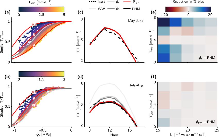
4260                     B. P. Sloan et al.: Plant hydraulic transport controls transpiration sensitivity to soil water stress

self, and the terms “β function” and “β factor” to refer to       Sabot et al., 2020) as well as soil water dynamics (Kennedy
the empirical function and its values, respectively.) The term    et al., 2019) compared to β. PHMs also exhibit more realistic
“well-watered” refers to moist soil conditions where stom-        sensitivity to atmospheric moisture demand than β (Liu et al.,
atal aperture is unaffected by plant water uptake from the        2020). However, these improvements from PHMs come at
soil, i.e., no soil water stress. The first β-like function ap-   the cost of an increased number of plant hydraulic trait pa-
peared, to the best of our knowledge, in an early global          rameters and computational burden, which can reduce the re-
heat balance study (Budyko, 1956) to reduce “evaporabil-          liability of the predictions (Prentice et al., 2015). Addition-
ity” (comparable to well-watered gs and T ) for unsaturated       ally, obtaining representative plant hydraulic trait values for
land surfaces using a normalized soil moisture value. This        a soil–plant system is difficult for two main reasons: (i) traits
method was eventually incorporated into the hydrology com-        vary widely across and within species (Anderegg, 2015) and
ponent of one of the first global circulation models (Manabe,     exhibit plasticity through acclimation and adaptation (Franks
1969). However, many current β functions appear to stem           et al., 2014), and (ii) trait measurements are typically made
from the heuristic root water uptake assumptions originally       at a single point (e.g., stem, branch, leaf), which may not
implemented in the crop transpiration model SWATR (Fed-           reliably scale to represent whole-plant or ecosystem-level re-
des et al., 1976, 1978), which evolved into the widely used       sponses due to the effects of nonlinear trait variations along
SWAP model (Kroes et al., 2017). Since then, β has gained         the soil–plant system (Couvreur et al., 2018). These difficul-
widespread use within TBMs and hydrological models due            ties result in uncertainty in the model predictions that may
to its parsimonious form.                                         be further compounded at the ecosystem level (Fisher et al.,
   However, mounting evidence indicates that using β in           2018; Feng, 2020). Consequently, modelers continue to rely
TBMs is a major source of uncertainty and bias in plant-          on β as a parsimonious alternative to PHMs (Paschalis et al.,
mediated carbon and water flux predictions. Multiple stud-        2020).
ies have implicated the lack of a universal β formulation as a       The relative strengths and weaknesses of β and PHMs sug-
primary source of inter-model variability in carbon cycle pre-    gest that informed model selection requires a better under-
dictions (Medlyn et al., 2016; Rogers et al., 2017; Trugman       standing of when the complexity of a PHM is justified over
et al., 2018; Paschalis et al., 2020). For example, different     the simplicity of β. This paper informs such understanding
β formulations among nine TBMs accounted for 40 %–80 %            by (i) analyzing the fundamental differences between PHMs
of inter-model variability in global gross primary productiv-     and β (Sect. 3.1), (ii) defining the parameters controlling the
ity (GPP) predictions (on the order of 3 %–286 % of current       differences (Sect. 3.2), and (iii) demonstrating how PHMs
global GPP) (Trugman et al., 2018). Aside from the uncer-         outperform β for a real soil–plant system (Sect. 3.3). Then,
tainty in functional form, β appears to fundamentally mis-        leveraging our theoretical insights, we create a new “dynamic
represent the coupled effects of soil water stress and atmo-      β” as a potential tool to correct the biases from the original
spheric moisture demand on stomatal closure. Recent work          β while reducing the parameter and computational demands
using model–data fusion at FLUXNET sites highlighted that         of PHMs (Sect. 3.3). To accomplish these goals, we first ana-
β produces stomatal responses that are overly sensitive to soil   lyze a minimalist PHM using a water supply–demand frame-
water stress and unrealistically insensitive to atmospheric       work, then corroborate the results for a more widely used
moisture demand (Liu et al., 2020). Furthermore, TBM vali-        complex PHM, and, finally, perform a case study with a cal-
dation experiments have found that β schemes produce unre-        ibrated land surface model (LSM), which employs β, PHM,
alistic GPP prediction during drought at Amazon rainforest        and dynamic β downregulation schemes.
sites (Powell et al., 2013; Restrepo-Coupe et al., 2017) and
systematic overprediction of evaporative drought duration,
magnitude, and intensity at several AmeriFlux sites (Ukkola       2     Methods
et al., 2016). The apparent inadequacy of β has lead to the
adoption of physically based plant hydraulic models (PHMs)        2.1    Minimalist PHM
in TBMs (Williams et al., 2001; Bonan et al., 2014; Xu et al.,
2016; Kennedy et al., 2019; Eller et al., 2020; Sabot et al.,     Our minimalist (Sect. 3.1–3.2) and complex PHM formu-
2020).                                                            lations (Sect. 3.3), illustrated in Fig. 1, rely on a supply–
   PHMs represent water transport, driven by a gradient of        demand framework that conceptualizes transpiration as the
water potential energy, through the soil–plant–atmosphere         joint outcome of soil water supply and atmospheric mois-
continuum via flux-gradient relationships (based on Hagen–        ture demand (Gardner, 1960; Cowan, 1965; Sperry and Love,
Poiseuille flow), which use measurable soil properties and        2015; Kennedy et al., 2019). In this framework, “supply”
plant traits as parameters (Mencuccini et al., 2019). The im-     refers to the rate of water transport to the leaf mesophyll
plementation of PHMs in several popular TBMs (e.g., CLM,          cells from the soil, into the roots, and through the xylem.
JULES, etc.) has improved predictions in site-specific GPP        “Demand” refers to the rate of water vapor outflux through
and evapotranspiration (ET) predictions (Powell et al., 2013;     the stomata, driven by the transport capacity of the air sur-
Bonan et al., 2014; Kennedy et al., 2019; Eller et al., 2020;     rounding the plant and regulated by the stomatal response to

Hydrol. Earth Syst. Sci., 25, 4259–4274, 2021                                      https://doi.org/10.5194/hess-25-4259-2021
B. P. Sloan et al.: Plant hydraulic transport controls transpiration sensitivity to soil water stress 4261
atmospheric conditions (Buckley, 2017) and leaf water status (similar to the approach of Jarvis, 1976) captures the ob-
(Klein, 2014; Buckley, 2019). We assume steady-state tran- served non-unique relationship between gs and ψl (Anderegg
spiration fluxes (i.e., supply equals demand), which means and Venturas, 2020) while facilitating comparison with the
we neglect the effects of plant capacitance (Bohrer et al., similar minimalist β formulation (see Sect. 2.5).
2005) and also assume that the mean plant and atmospheric
states equilibrate quickly over short timescales. Td = LAI · f (ψl ) · gs,ww · D · Ca = f (ψl ) · Tww · Ca ; (2)
The minimalist PHM supply (Ts [mm d−1 ]; Eq. 1 and blue
1 ψl ≥ ψl,o ,
segment in Fig. 1a) is represented by a steady-state inte- gs (ψl ) ψl,c −ψl
f (ψl ) = = ψ −ψ ψl,c < ψl < ψl,o , (3)
grated 1-D flux-gradient relationship, bounded by the root- gs,ww l,c l,o
zone-average soil water potential (ψs [MPa]) and leaf water 0 ψl ≤ ψl,c .
potential (ψl [MPa]) and mediated by the bulk conductance
along the flow path (gsp (ψ) [mm d−1 MPa−1 ]). For simplic- The PHM supply and demand are coupled through their
ity, we assume constant soil–plant conductance (gsp ) and ig- mutual dependence on leaf water potential. The ψl value that
nore its dependence on water potential (i.e., hydraulic limits; balances supply (Eq. 1) and demand (Eq. 2) – which we will
Sperry et al., 1998). This assumption simplifies the integral call ψl∗ (Eq. 4) – yields the steady-state transpiration rate for
in Eq. (1) to the product of gsp and the water potential differ- the minimalist PHM (T phm ; Eq. 5). The full derivation of ψl∗
ence, ψs − ψl , which drives the flow. and T phm is shown in Sect. S1 in the Supplement.
T ·ψ
Zψl ψs · ψl,o − ψl,c + wwgsp l,c
ψl∗ = ; (4)
Ts = − gsp (ψ) dψ = gsp · (ψs − ψl ) (1) ψl,o − ψl,c + Tgww
sp
ψs
ψs > ψl,o + Tgww
T ,
ww
sp
The minimalist PHM demand (Td [mm d−1 ]; Eq. 2 and phm ( ψ l,c −ψ s)
ψl,c < ψs ≤ ψl,o + Tgww
T = Tww · ,
(ψl,c −ψl,o )− Tgww sp
red segment in Fig. 1a) uses a similar conductance-difference
sp
0
ψs ≤ ψl,c .
formulation (i.e., integrated flux-gradient relationship). Tran-
(5)
spiration is driven by the leaf-to-air water vapor pressure
deficit (D [mol H2 O per mol air]) and mediated by the well- 2.2 Complex PHM
watered stomatal conductance (gs,ww [mol air m−2 s−1 ]), a
stomatal closure term (f (ψl )), and the leaf area index (LAI The LSM analysis (Sect. 3.3) uses a complex PHM formula-
[m2 leaf m−2 ground]). Additionally, we convert Td from a tion following Feng et al. (2018). The PHM separates supply
molar flux to a volume flux using the conversion factor Ca into soil-to-xylem and xylem-to-leaf segments and demand
(i.e., the molar weight of water (Mw [kg mol−1 ]) divided by into a leaf-to-atmosphere segment (Fig. 1b). Here, we briefly
water density (ρw [kg m−3 ]) and multiplied by the conversion discuss the complex PHM components for a single big-leaf
from m s−1 to mm d−1 ). The driving force D assumes satura- formulation; however, we refer the reader to Sects. S2–S3 for
tion vapor pressure inside the leaf (i.e., ei = esat ) and that the full model details and parameter values for the two-big-leaf
leaf surface (es ) and atmospheric vapor pressure (ea ) are the formulation used in our LSM.
same (i.e., the leaf is well-coupled to the atmosphere; Jarvis For PHM supply (Ts ; blue segments in Fig. 1b), the wa-
and McNaughton, 1986); however, the leaf temperature can ter potential gradient drives flow through the soil–plant sys-
differ from the atmosphere, which differentiates D from at- tem mediated by the segment-specific conductances. Unlike
mospheric vapor pressure deficit (Grossiord et al., 2020). The the minimalist PHM (Sect. 2.1), we assume the conductance
parameter gs,ww encapsulates the stomatal response to at- in each segment depends on water potential, which repre-
mospheric conditions only (i.e., light, temperature, humid- sents “hydraulic limits” (Sperry et al., 1998) that arise via
ity, and CO2 concentration). We define the product of LAI, (i) the inability of roots to remove water from soil pores at
gs,ww , and D as the well-watered transpiration rate (Tww ) – low ψs and (ii) xylem embolism caused by large hydraulic
which represents atmospheric moisture demand throughout gradients required under low ψs and/or high Tww . The soil-
this paper – and we specify its value for the minimalist anal- to-xylem conductance (gsx [mm d−1 MPa−1 ]; Eq. 6 and illus-
ysis. The term “well-watered” refers to abundant soil water trated in Fig. 1b) is its maximum value (gsx,max ) downreg-
conditions under which water transport to the leaves main- ulated by the unsaturated soil hydraulic conductivity curve
tains ψl high enough to avoid stomatal closure. During water- (Clapp and Hornberger, 1978), which is parametrized by
stressed conditions, the f (ψl ) term represents stomatal clo- the saturated soil water potential (ψsat ), soil water retention
sure (i.e., downregulating gs,ww ) to lowering leaf water status exponent (b), unsaturated hydraulic conductivity exponent
(Buckley, 2019). We assume a normalized, piecewise linear (c = 2b + 3), and a correction factor (d) to account for roots’
f (ψl ) (Eq. 3 and illustrated in Fig. 1a), parametrized by the ability to reach water (Daly et al., 2004). The xylem-to-
leaf water potential at incipient (ψl,o ) and complete stomatal leaf conductance (gxl [mm d−1 MPa−1 ]; Eq. 7 and illustrated
closure (ψl,c ). This simple multiplicative reduction of gs,ww in Fig. 1b) is its maximum value (gxl,max ) downregulated
https://doi.org/10.5194/hess-25-4259-2021 Hydrol. Earth Syst. Sci., 25, 4259–4274, 2021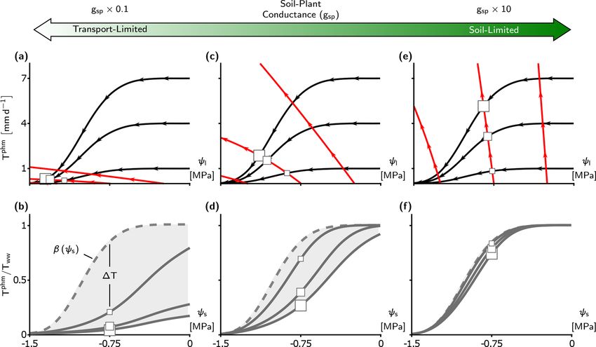
4262 B. P. Sloan et al.: Plant hydraulic transport controls transpiration sensitivity to soil water stress
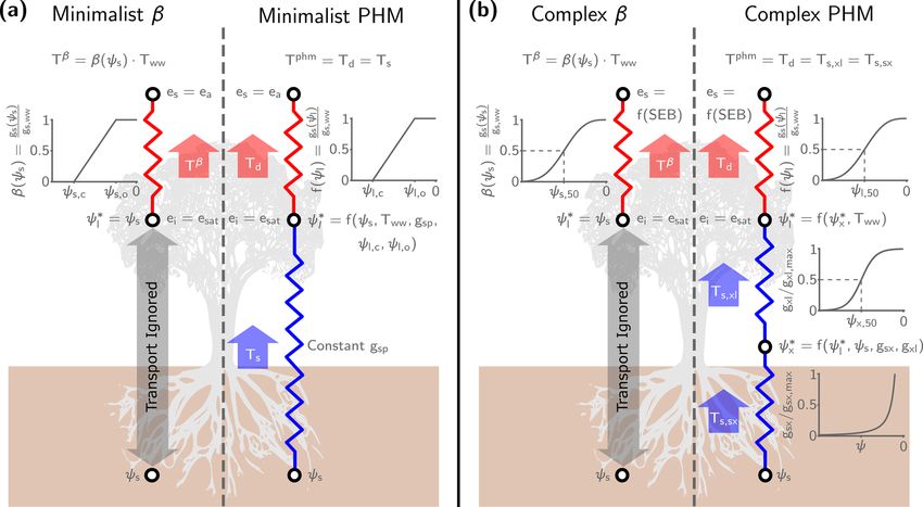
Figure 1. Schematic for the minimalist (a) and complex (b) β and PHM models used in this analysis. The resistors represent the conductance
between soil–plant segments (i.e., an analogy to Ohm’s law) that mediate liquid water supply (blue) and atmospheric water vapor demand
(red). Next to each resistor is the segment-specific conductance downregulation curve dependent on water potential (ψ). The white circles
indicate segment endpoints where we calculate the potentials (ψ) for liquid water transport and vapor pressures (e) for water vapor transport.
The supply segment subscripts represent soil (s), xylem (x), leaf (l), and bulk soil-plant (sp), whereas the demand segment subscripts represent
inside the leaf (i), at the leaf surface (s), and the ambient air (a). For water vapor transport, we assume saturation vapor pressure inside the
leaf (ei = esat ) for both models. In the minimalist models, we assume the leaf surface vapor pressure (es ) is the atmospheric vapor pressure
(ea ), which makes the driving force for water vapor transport the leaf-to-air vapor pressure deficit (D = esat −ea ). Alternately, in the complex
models, es is a function of the surface energy balance (f (SEB)) calculations at each time step. The thick arrows represent the water transport
through each segment calculated by the integrated steady-state flux-gradient relationships discussed in Sect. 2.1–2.2 and 2.5. We use the
minimalist models (left panel) for Sect. 3.1–3.2 and the complex models (right panel) for the LSM analysis in Sect. 3.3. (Note that we only
illustrate a single big-leaf formulation here, but see Sect. S2 for the two-big-leaf implementation.)
by a sigmoidal function (Pammenter and Willigen, 1998),
1
which is parametrized by the vulnerability exponent (a) and gxl (ψ) = gxl,max · 1 − , (7)
the xylem water potential (ψx ) at 50 % loss of conductance 1 + ea·(ψ−ψx,50 )
(ψx,50 ). We estimate the maximum conductance values for Zψ
g ψ 0 dψ 0 ,
each segment (gsx,max and gxl,max ) with trait-based equations 8(ψ) = (8)
following Feng et al. (2018) (see Sect. S2.5.3). Given that −∞
conductance varies with water potential, we utilize a Kirch- Ts,sx = 8sx (ψs ) − 8sx (ψx ), (9)
hoff transform (Eq. 8) to approximate the water supply from
Ts,xl = 8xl (ψx ) − 8xl (ψl ). (10)
each segment (Ts,sx and Ts,xl [mm d−1 ]; Eqs. 9–10) as the
difference in the matric flux potential (8 [mm d−1 ]) at the The complex PHM demand (Td [mm d−1 ]; Eq. 11 and red
segment endpoints. Therefore, given a value of ψs (i.e., root- segment in Fig. 1b) mirrors the minimalist version (Eq. 2)
zone-average water potential) and ψl , the ψx that balances with modifications to fit into a dual-source LSM scheme
Ts,sx and Ts,xl – called ψx∗ – yields the steady-state supply (Sect. 2.3) that explicitly represents the coupled mass, heat
rate (Ts ). and energy transfer between the plant, its microclimate, and
c−d the atmosphere. The driving force of transpiration is no
ψsat b
longer D (i.e., the leaf-to-air vapor pressure deficit) but rather
gsx (ψ) = gsx,max · , (6)
ψ the difference between leaf internal (ei [kPa]) and surface (es
[kPa]) vapor pressure (normalized by atmospheric pressure
Hydrol. Earth Syst. Sci., 25, 4259–4274, 2021 https://doi.org/10.5194/hess-25-4259-2021B. P. Sloan et al.: Plant hydraulic transport controls transpiration sensitivity to soil water stress 4263
(Patm [kPa]) to obtain units mol H2 O per mol air). We still mass, heat, or energy storage), (ii) neutral atmospheric sta-
assume ei is the saturation vapor pressure at leaf temperature bility, (iii) implemented the Goudriaan and van Laar (1994)
(esat ), but now es depends on the plant microclimate deter- radiative transfer model in lieu of the two-stream approx-
mined by the LSM energy balance solution at each time step imation (Oleson et al., 2018), and (iv) forced the LSM
(see Sect. S2.6). This plant microclimate is coupled to the with soil moisture, soil heat flux, and downwelling radia-
well-watered stomatal conductance (gs,ww [mol air m−2 s−1 ]) tion data. We refer the reader to Sect. S2 for full model
via the optimality-based stomatal response model of Medlyn details and justifications. We formulated the LSM in MAT-
et al. (2011). The Medlyn model (Eq. 12) depends on the leaf LAB and have made our codes available online (Sloan, 2021;
vapor pressure difference (ei − es [kPa]), net CO2 assimila- https://doi.org/10.5281/zenodo.5129247).
tion rate (An [mol CO2 m−2 s−1 ]), and the leaf surface CO2 We created separate LSM versions to test five different
mole fraction (approximated by the ratio of leaf surface CO2 transpiration downregulation schemes: (i) well-watered (no
partial pressure (cs [kPa]) and Patm to give units mol CO2 downregulation), (ii) a single β (βs ) with static parameters,
per mol air) and is parametrized by the minimum stomatal (iii) a β separately applied to sunlit and shaded leaf areas
conductance (go [mol air m−2 s−1 ]) and a slope parameter (β2L ) with static parameters, (iv) a dynamic β with parame-
(g1 [kPa0.5 ]). Furthermore, we couple gs,ww to the Farquhar ters dependent on Tww (βdyn ), and (v) a PHM. We calibrated
et al. (1980) photosynthesis model through An to ensure CO2 the PHM version using a two-step approach. First, we sim-
diffusion into the leaf balances carbon assimilation (Collatz ulated 13 600 parameter sets using Progressive Latin Hyper-
et al., 1991) (see Sect. S2.4). As in the minimalist model, cube Sampling (Razavi et al., 2019) on 15 soil and plant pa-
the product of gs,ww , driving force, and LAI yields the well- rameters (Table S6) and selected the best parameter set based
watered transpiration rate, Tww , which we take to represent on a comparison of RMSE, correlation coefficient, percent
atmospheric moisture demand. Under water-stressed condi- bias, and variance to AmeriFlux evapotranspiration, sensi-
tions, we keep a Jarvis-like stomatal closure term (f (ψl )) to ble heat flux, gross primary productivity, and net radiation
downregulate gs,ww , because it facilitates easy comparisons site data (Figs. S5–S8). Unfortunately, the best parameter set
between our minimalist and complex formulations. However, contained an unrealistically low ψl,50 value for ponderosa
we upgrade f (ψl ) from a piecewise linear form (Eq. 3) to a pine compared to observations (DeLucia and Heckathorn,
more realistic Weibull form (Eq. 13 and illustrated in Fig. 1b) 1989). Therefore, as a second step, we adjusted the ψl,50
parametrized by a shape factor describing stomatal sensitiv- and several other soil and plant parameters to more realistic
ity (bl ) and the leaf water potential at 50 % loss of stom- values while ensuring that they replicated the transpiration
atal conductance (ψl,50 [MPa]) (Klein, 2014; Kennedy et al., downregulation behavior of the original parameter set. These
2019). parameter adjustments had minimal impact on the LSM pre-
ei − es dictions as the underlying equations are highly nonlinear, and
Td = LAI · f (ψl ) · gs,ww · · Ca = f (ψl ) · Tww · Ca , (11) multiple parameter sets can give near equivalent results (i.e.,
Patm
g1
1.6 · An equifinality). We refer the reader to Sect. S4 for a more de-
gs,ww = go + 1 + √ · , (12) tailed account of calibration.
ei − es cs /Patm
b We parametrized the three LSM versions containing the
ψl l
gs (ψl ) − ψl,50 β schemes by calibrating the respective β functions to the
f (ψl ) = =2 . (13)
gs,ww relative transpiration outputs (T /Tww ) of the calibrated PHM
As in the minimalist PHM, the complex PHM supply and version, while we ran the well-watered version using the cali-
demand are coupled through their mutual dependence on ψl . brated parameters and downregulation turned off. The choice
The ψl∗ that balances Ts (found at ψx∗ for Eqs. 9–10) and Td to calibrate a single LSM version ensured that the perfor-
(Eq. 11) yields the steady-state transpiration rate for the com- mance differences between the schemes would be due to the
plex PHM (T phm ). We numerically calculate this solution by PHM representing plant water use more realistically and not
recasting Eqs. (9)–(11) as a nonlinear least squares problem to the artifact of differing parameter fits between LSM ver-
and finding the ψl∗ and ψx∗ that ensure mass balance between sions. We refer the reader to Sect. S6.2 for specific details of
the segments (see Sect. S2.5.3). the parameter fits for the β schemes.
2.3 LSM description and calibration 2.4 Site description and forcing data
We created an LSM to test several transpiration downregu- We calibrated and forced the LSM with half-hourly data
lation schemes (Sect. 3.3) and allow for removal of modules from the US-Me2 “Metolius” AmeriFlux site (Irvine et al.,
(e.g., subsurface heat and mass transfer) that would unnec- 2008) for daylight hours during May-August 2013-2014. The
essarily complicate our comparisons. Our LSM is a dual- forcing data were taken from both the AmeriFlux (Law,
source two-big-leaf approximation (Bonan, 2019) adapted 2021) and FLUXNET2015 (FLUXNET2015, 2019; Pas-
from CLM v5 (Oleson et al., 2018) with several key sim- torello et al., 2020) data products (see Sect. S5 for full de-
plifications: (i) steady-state conditions (i.e., no aboveground tails). The site consists of intermediate-age ponderosa pine
https://doi.org/10.5194/hess-25-4259-2021 Hydrol. Earth Syst. Sci., 25, 4259–4274, 20214264 B. P. Sloan et al.: Plant hydraulic transport controls transpiration sensitivity to soil water stress
trees on sandy loam soil in the Metolius River basin in Ore- In this paper, we have defined the β function in terms of
gon, USA. We selected this site specifically for its subsur- ψs and apply the β factor directly to gs,ww and, in turn, Tww
face soil moisture and temperature profiles as well as its (Eq. 14) for three key reasons: (i) water transport through the
separate measurements of photosynthetically active radia- soil–plant–atmosphere continuum follows a gradient of wa-
tion (PAR) and near-infrared radiation (NIR). We used these ter potential, not water content, (ii) β using ψs rather than θs
boundary condition data to force the LSM in lieu of solving produces more realistic downregulation behavior compared
one-dimensional subsurface mass and heat transfer equations to data (Verhoef and Egea, 2014), and (iii) applying the β fac-
and atmospheric radiation partitioning models. In particular, tor to gs,ww directly corresponds to the PHM demand in both
we forced the LSM with root-zone-averaged soil water po- minimalist and complex formulations. In the minimalist anal-
tential (ψs ; estimated from measured soil water content and ysis (Sect. 3.1–3.2), β(ψs ) (Eq. 15 and illustrated in Fig. 1a)
a pedotransfer function) and the ground heat flux measure- takes a piecewise linear form (analogous to Eq. 3), which is
ments. We selected the measurement depth of 50 cm to rep- parametrized by the soil water potential at incipient (ψs,o )
resent ψs based on the deviation of measured GPP from its and complete stomatal closure (ψs,c ). Similarly, in the LSM
mean in relation to measured soil water content and vapor analysis (Sect. 3.3), β(ψs ) (Eq. 16 and illustrated in Fig. 1b)
pressure deficit (Fig. S10). The 50 cm measurements showed takes a Weibull form (analogous to Eq. 13) parametrized by
clear GPP downregulation under water stress. Furthermore, the soil water potential at 50 % loss of stomatal conductance
the depth seemed reasonable given previous modeling at this (ψs,50 ) and a stomatal sensitivity parameter (bs ). The LSM
site estimated an effective rooting depth of 1.1 m (Schwarz analysis uses two versions of Eq. 16: (i) a static version with
et al., 2004). The atmospheric forcing for the LSM consisted constant bs and ψs,50 (used by the βs and β2L schemes) and
of incoming direct and diffuse NIR and PAR fluxes, CO2 (ii) a dynamic version where bs and ψs,50 are linear func-
concentration, atmospheric pressure, vapor pressure, temper- tions of Tww (used by the βdyn scheme). We refer the reader
ature, and wind velocity at the measurement tower height of to Fig. S12 for illustrations of the different β versions.
32 m. Full description of the forcing data is given in Sect. S5.
T β = β (ψs ) · Tww ; (14)
2.5 β formulations
1
ψs ≥ ψs,o ,
ψs,c −ψs
The β function empirically represents stomatal closure to de- β (ψs ) = ψs,c < ψs < ψs,o , (15)
ψs,c −ψs,o
clining leaf water status caused by soil water stress. By de- 0 ψs ≤ ψs,c ;
sign, β makes the simplifying assumption that stomata re-
ψs
bs (Tww )
− ψs,50 (Tww )
spond directly to soil water status (to avoid the complexity β(ψs , Tww ) = 2 . (16)
of implementing a PHM as illustrated by Fig. 1), which is
readily available in TBM subsurface hydrology schemes as
ψs or volumetric soil water content (θs ). This heuristic ap- 3 Results
proach leads to multiple β functions based on modeler pref-
3.1 β as a limiting case of PHMs with infinite
erence (see the supplement of Trugman et al., 2018, for a
conductance
list of differing β formulations common to TBMs). Further-
more, even if a universal β function existed, there is open The supply–demand framework reveals that the minimalist
debate on how to apply the β factor (Egea et al., 2011); some PHM and β fundamentally differ in their coupling of the ef-
TBMs apply the β factor directly to stomatal conductance fects of soil water stress (represented by ψs ) and atmospheric
(Kowalczyk et al., 2006; De Kauwe et al., 2015; Wolf et al., moisture demand (represented by Tww ) on transpiration. The
2016), whereas others indirectly affect stomatal conductance PHM supply lines (red lines in Fig. 2a) illustrate soil-to-leaf
by applying the β factor to photosynthetic parameters (Zhou water transport (Eq. 1) at a fixed soil water availability (ψs )
et al., 2013; Lin et al., 2018; Kennedy et al., 2019). Here, under increasing pull from the leaf (lower ψl ) and constant
we select a single β formulation that easily compares with soil–plant conductance (gsp ; supply line slope). The PHM de-
the demand component of our PHM. Selecting a different β mand lines (black lines in Fig. 2a) illustrate transpiration re-
formulation could alter our values; however, we do not ex- duction under lower ψl (from stomatal closure) for two Tww
pect our main conclusions about β and PHM differences to values. The supply and demand lines intersect at the mini-
change as long as two criteria are met. First, the stomatal malist PHM solution (ψl∗ and T phm ; Eqs. 4–5). Therefore,
downregulation factors for the PHM (f (ψl )) and β (β(ψs )) the minimalist PHM couples the effects of soil water stress
are applied consistently in the transpiration downregulation to atmospheric moisture demand on transpiration downregu-
scheme (to either gs,ww or photosynthetic parameters). Sec- lation, because leaf water potential responds to ψs and Tww
ond, if β is in terms of θs , a curvilinear form must be used until it reaches the point of steady-state transpiration (i.e.,
(Egea et al., 2011) to ensure β can be mapped approximately T phm (ψl∗ ) = Ts (ψl∗ ) = Td (ψl∗ )).
to the water potential space of our analysis. The minimalist β transpiration rate (T β ; Eq. 14) ignores
this coupling as the β function depends only on ψs and
Hydrol. Earth Syst. Sci., 25, 4259–4274, 2021 https://doi.org/10.5194/hess-25-4259-2021B. P. Sloan et al.: Plant hydraulic transport controls transpiration sensitivity to soil water stress 4265
Figure 2. Fundamental differences between minimalist PHM and β. (a–b), Supply (red) and demand (black) curves for PHM (a, solid lines)
and β (b, dashed lines) under varying leaf water potentials (ψl ). The squares (circles) represent the PHM (β) solution – i.e., the ψl∗ where
supply equals demand – for a single soil water availability (ψs ) and two atmospheric moisture demands (Tww ). These markers carry through
panels (c) and (d) to illustrate how the solutions between the PHM and β diverge at a single ψs . The relative size of the markers indicates
corresponding Tww . The water potential difference 1ψ required to transport water from soil to leaf is shown in panel (a) for ψs = −1 MPa
and Tww = 10 mm d−1 . (c) Solutions of panels (a) and (b) mapped to ψs , where 1T is the difference between PHM and β transpiration
estimates at ψs = −1 MPa and Tww = 10 mm d−1 . (d) Relative transpiration, in which solutions in panel (c) are normalized by Tww . The β
solutions collapse to a single curve, whereas the PHM solutions depend on Tww .
independently reduces Tww (shown in Fig. 1). The condi-
tions leading to the decoupling in β only arise if the sup- lim (1T ) = lim T phm − T β = lim
gsp →∞ gsp →∞ gsp →∞
ply lines are vertical (Fig. 2b), which results in the relative
transpiration (T β /Tww ) depending on ψs only (single curve ψl,c − ψs ψl,c − ψs
Tww · − = 0. (18)
in Fig. 2d). Since gsp is the supply line slope (Eq. 1), β ψl,c − ψl,o − Tgww
ψl,c − ψl,o
sp
represents a limiting case of the PHM in which the soil–
plant system is infinitely conductive. More specifically, as The PHM coupling results in greater transpiration down-
gsp increases, the leaf water potential approaches the soil regulation compared to β under the same environmental con-
water potential (ψl∗ → ψs ; Eq. 17) and the PHM transpira- ditions (Fig. 2c). For a given soil water stress (ψs ), β assumes
tion rate approaches the β transpiration rate (T phm → T β ; ψs = ψl∗ and downregulates any atmospheric moisture de-
Eq. 18). Therefore, the β(ψs ) function (Eq. 15) equals the mand (Tww ) value by a fixed proportion (i.e., it scales lin-
f (ψl ) function (Eq. 3) in PHMs and represents stomatal clo- early with Tww ); hence, it can be modeled with a single curve
sure to declining leaf (or soil) water potential. In summary, (Fig. 2d). Conversely, the PHM (with finite conductance) re-
the empirical β physically represents an infinitely conductive quires a water potential difference (1ψ = ψs − ψl∗ ) to trans-
soil–plant system where stomata close in response to leaf wa- port water from soil to leaf; therefore, ψl∗ must be less than
ter potential that depends solely on the soil water potential ψs , and greater stomatal closure results (Fig. 2c). Further-
with which it is equilibrated. more, the PHM downregulates transpiration at a greater pro-
T ·ψ portion with increasing Tww (i.e., it scales nonlinearly with
ψs · ψl,o − ψl,c + wwgsp l,c
lim ψl∗
= lim = ψs (17) Tww ) as it requires a greater 1ψ and lower ψl∗ (Fig. 2d).
ψl,o − ψl,c + Tgww
gsp →∞ gsp →∞ Hence, PHMs require transpiration downregulation to be de-
sp
scribed as a function of both ψs and Tww .
These minimalist model results suggest that the range
of soil–plant conductances (gsp ) can generate a spectrum
https://doi.org/10.5194/hess-25-4259-2021 Hydrol. Earth Syst. Sci., 25, 4259–4274, 20214266 B. P. Sloan et al.: Plant hydraulic transport controls transpiration sensitivity to soil water stress
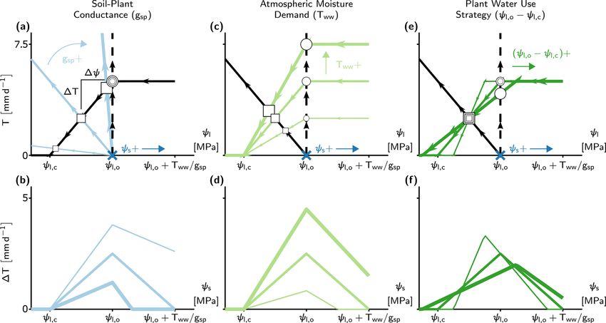
Figure 3. The effect of soil water potential (ψs ), soil–plant conductance (gsp ), atmospheric moisture demand (Tww ), and plant water use
strategy (ψl,o − ψl,c ) on differences between the minimalist PHM and β models (1T ). (a, c, e) Supply–demand curves at a single soil water
availability (indicated by the dark blue x at ψs = ψl,o ) for three prescribed values of gsp , Tww , and ψl,o − ψl,c , respectively. Each parameter
(gsp , Tww , or ψl,o − ψl,c ) is set at 50 % above (below) its base values at gsp = 10 mm d−1 MPa−1 , Tww = 5 mm d−1 , ψl,o = −1 MPa, and
ψl,c = −2 MPa using thick (thin) colored lines. The squares (circles) indicate the PHM (β) solutions, with size corresponding to magnitude
of the changing parameter values. Note that the vertical distance between a correspondingly sized circle and square is 1T , and horizontal
distance is 1ψ. (b, d, f) The 1T results from panels (a), (c), and (e) calculated for a range of ψs with line thickness proportional to
parameters in the aforementioned panels (e.g., thick blue line in panel b corresponds to 50 % increase in gsp shown in panel a). The x axes
are mapped from ψl in the top panels to ψs in the bottom panels.
of possible transpiration responses to soil water stress (and ψl,c < ψs < ψl,o + Tww /gsp ) (Fig. 3b, d, f). The peak 1T
atmospheric moisture demand). Two classes of behaviors occurs at the incipient point of stomatal closure (ψl,o ) as
emerge – one in a “soil-limited” soil–plant system, in which (i) when ψs < ψl,o , transpiration begins to decrease, and in
gsp is large enough for ψl ≈ ψs , thus decoupling the ef- its extreme limit, transpiration (and thus 1T ) approaches 0,
fects of soil water stress and atmospheric moisture demand and (ii) when ψs > ψl,o , the effects of downregulation di-
while allowing the relative transpiration to vary only with ψs minish in both models as the soil becomes well-watered. The
(Fig. 2d). The other class of behavior arises in “transport- 1T –ψs behavior acts as a baseline relationship in the follow-
limited” systems with finite gsp , in which a non-negligible ing analysis of gsp , Tww , and ψl,o − ψl,c controls.
water potential difference (1ψ) is required to transport the The 1T –ψs relationship increases with lower gsp (Fig. 3b;
water to the leaf, resulting in additional downregulation com- greater transport limitation) because flatter supply lines in-
pared to soil-limited systems (Fig. 2c) and requiring relative crease 1ψ (Fig. 3a), requiring greater stomatal closure and
transpiration to depend on both ψs and Tww (Fig. 2d). hence additional downregulation for a PHM compared to
β. Similarly, higher Tww increases the 1T –ψs relationship
3.2 Parameters controlling the divergence of β and (Fig. 3d), although the increase in 1ψ stems from steeper
PHMs demand line slope (Fig. 3c). In addition to increasing 1T at
each ψs value, the effects of gsp and Tww increase the range
The differences in PHM and β transpiration estimates (1T ) of soil water stress above ψl,o (up to saturated soil water po-
depend not only on gsp but also on soil water availability tential). This result indicates that PHMs can simulate tran-
(ψs ), atmospheric moisture demand (Tww ), and plant wa- spiration downregulation under moist soil conditions that β
ter use strategy (ψl,o − ψl,c ). To disentangle these joint de- potentially misses as it does not account for large 1ψ values
pendencies, we adjust a single variable and explore the im- from transport limitation and/or high atmospheric moisture
pact on 1T using the supply and demand lines (Fig. 3). demand. Finally, as gsp increases (soil-limited) and Tww de-
The translation of supply lines represents ψs changes (indi- creases, 1T tends to zero, once again, for slightly different
cated in Fig. 3a, c, e) and produces a non-monotonic rela- reasons: for gsp , the supply lines approach the β assumption
tionship with 1T over the range of soil water stress (i.e.,
Hydrol. Earth Syst. Sci., 25, 4259–4274, 2021 https://doi.org/10.5194/hess-25-4259-2021B. P. Sloan et al.: Plant hydraulic transport controls transpiration sensitivity to soil water stress 4267
(vertical dashed line in Fig. 3a), whereas for Tww , transpira- tential differences (1ψ) creating large differences between
tion approaches zero. PHMs and β (high 1T ) at intermediate ψs values (Fig. 4b,
Lastly, we explore the effect of plant water use strategy d). Second, for a transport-limited system, 1T increases with
(ψl,o − ψl,c ) on 1T – which approximates the sensitivity of higher variability in atmospheric moisture demand (Tww ),
stomatal closure to ψl . Altering ψl,o − ψl,c does not affect where the importance of “variability” expands on our min-
1ψ like the other three variables; however, it modifies the imalist results. To clarify, β should be considered an empiri-
range of soil water stress and redistributes 1T to conserve cal model that could be fit anywhere within the range of the
the total error over the range. For example, a more aggressive PHM downregulation envelope (light gray shading in Fig. 4b,
plant water use strategy – closing stomata over a narrower d, f). Therefore, greater Tww variability creates a larger PHM
range of ψl and ψs – creates a narrower range of soil water downregulation envelope and makes a single β increasingly
stress with a more peaked 1T –ψs relationship due to more inadequate for modeling transpiration downregulation.
vertical demand lines (Fig. 3e). Therefore, whether the plant The consistency between the minimalist and complex
water use strategy could amplify or diminish 1T for a soil– PHM suggests that the divergence between PHMs and β in
plant system relies on how site-specific soil moisture vari- transport-limited systems is not sensitive to the linear or non-
ability overlaps with the range of soil water stress (Fig. 3f). linear forms of supply or demand lines but is rather con-
In summary, this minimalist analysis suggests that PHMs trolled by the existence of a finite conductance itself. Fur-
are most needed to represent transport-limited soil–plant sys- thermore, these results strongly support the need to use two
tems under high atmospheric moisture demand and moderate independent variables, ψs and Tww (rather than only ψs in
soil water availability. Plant water use will modulate these β), to capture the coupled effects of soil water stress and at-
results; however, the impact depends on how site-specific mospheric moisture demand on transpiration downregulation
soil moisture variability overlaps with the range of soil water in transport-limited soil–plant systems. In light of these find-
stress. ings, we have developed a new dynamic β (βdyn ) that has an
additional functional dependence on Tww (Eq. 16) and com-
3.3 Improving transpiration predictions with a PHM pared it against four other downregulation schemes in this
and a dynamic β LSM analysis.
We now assess the errors incurred by using a β rather than
We now perform a modeling case study of the AmeriFlux PHM downregulation scheme to model the US-Me2 pon-
US-Me2 ponderosa pine site (Sect. 2.4) using our own cali- derosa pine site. The median diurnal evapotranspiration (ET;
brated LSM (Sect. 2.3) with five separate transpiration down- bare soil evaporation plus transpiration) for each LSM ver-
regulation schemes: (i) well-watered (no downregulation), sion for early summer 2013–2014 indicates that all down-
(ii) single β (βs ), (iii) β separately applied to sunlit and regulation schemes perform similarly due to high soil mois-
shaded leaf areas (β2L ), (iv) βdyn , and (v) PHM. Specifically, ture and minimal downregulation (Fig. 5c). However, as soil
we aim to (i) verify the transport-limitation spectrum from moisture declines during late summer (Fig. S11) the differ-
the minimalist analysis (Sect. 3.1) for a complex PHM for- ences between schemes emerge: the PHM and βdyn schemes
mulation common to TBMs, (ii) identify errors incurred by fit the ET observations the best, while β2L , βs , and well-
selecting β over a PHM (Sect. 3.2) for a real transport-limited watered schemes overpredict ET (Fig. 5d). We explain the
soil–plant system, and (iii) develop a new dynamic β that ap- poor performance of the static β schemes by plotting the re-
proximates a PHM with simple modifications to the existing duction in absolute percent bias between the βs and PHM
β. schemes (Fig. 5e) with respect to soil water stress (repre-
To aid our comparison of LSM transpiration downregula- sented by volumetric soil water content measurements at the
tion schemes, we must first verify that the spectrum of trans- site, θs [m3 water per m3 soil]) and atmospheric moisture de-
port limitation found in our minimalist analysis (Sect. 3.1) mand (represented by Tww from the well-watered LSM ver-
adequately describes the differences between PHM and β sion). The PHM scheme provides substantial percent bias re-
formulations common to TBMs. Our calibrated LSM uses duction relative to the static βs scheme under soil water stress
a complex PHM formulation (Sect. 2.2 and Fig. 1b) that (θs < 0.2) for above- and below-average Tww values (Tww ≈
partitions the soil–plant–atmosphere continuum into soil-to- 4 mm d−1 ). This result is true for both static β schemes (βs
xylem, xylem-to-leaf, and leaf-to-atmosphere segments, each and β2L ), because they are fit to the average Tww behav-
with conductance curves that depend nonlinearly (e.g., sig- ior over the simulation period (Fig. 5a–b and Sect. S6.2).
moidal or Weibull) on water potential. This added com- Therefore, as Tww becomes higher (lower) than the average,
plexity does not affect the spectrum of transport limitation these static β schemes will overpredict (underpredict) tran-
(Fig. 4). For clarity, we reiterate two main points from the spiration. The PHM also improves performance during wet-
minimalist PHM analysis found in this complex analysis. ter soil conditions (θs > 0.2) with high Tww – which does
First, soil–plant conductance (gsp ) controls whether the soil– not represent typical “drought” conditions – suggesting that
plant system is soil-limited (high gsp ; Fig. 4e–f) or transport- PHMs capture transpiration downregulation that β poten-
limited (low gsp ; Fig. 4a–b) due to non-negligible water po- tially misses as it cannot account for large soil–plant water
https://doi.org/10.5194/hess-25-4259-2021 Hydrol. Earth Syst. Sci., 25, 4259–4274, 20214268 B. P. Sloan et al.: Plant hydraulic transport controls transpiration sensitivity to soil water stress
Figure 4. Transport-limitation spectrum observed in the complex PHM formulation. (a, c, e) Supply–demand curves for three values of soil–
plant conductance, gsp , using the complex PHM formulation. Panel (c) uses the calibrated LSM parameters from the US-Me2 AmeriFlux site
discussed in Sect. 2.3. Panels (a) and (e) contain the calibrated conductance (gsp ≈ 13 mm d−1 MPa−1 ) multiplied by 0.1 and 10, respectively.
The supply lines (red) are shown at ψs equal to 0, −0.75, and −1.5 MPa, and demand lines (black) are shown at Tww equal to 1, 4, and
7 mm d−1 . The PHM solution for ψs at −0.75 MPa is shown by the squares with size corresponding to Tww magnitude. (b, d, f) The relative
transpiration for the PHM (solid) in panels (a), (c), and (e) and the infinitely conductive β solution (dashed line) are shown. The light gray
shading indicates the PHM downregulation envelope bounded by β(ψs ) as Tww approaches zero and the relative transpiration curve at the
highest Tww .
potential differences (1ψ) under transport limitation and/or (Sect. S6.2). Furthermore, βdyn does not require the itera-
high atmospheric moisture demand (similar to Sect. 3.2). tive solution of water potentials and transpiration in PHMs
Lastly, the near-average Tww conditions lead to β providing (Sect. 2.2). Rather, it calculates transpiration downregulation
enhanced performance, which can be explained by underly- algebraically using ψs as in the original β. The βdyn provides
ing biases in the calibrated parameter estimates (see Fig. S9). a future avenue for correcting existing β model bias without
Notably, the βdyn downregulation scheme replicates the adding the computational and parametric challenges of more
performance of the PHM scheme by adding a single dimen- realistic PHMs.
sion of Tww to the original β scheme. This additional de-
pendence on Tww allows βdyn to traverse along the PHM
downregulation envelope with atmospheric moisture demand 4 Discussion and conclusion
changes, whereas the static β schemes are fixed near mean
conditions (Fig. 5a–b). The performance difference between The spectrum of transport- and soil-limited transpiration
PHM and βdyn schemes is minimal in terms of percent (Fig. 4) explains why many TBMs that use β to represent
change in bias across all environmental conditions (Fig. 5f; transpiration downregulation struggle to predict water, en-
max difference of 3 %), median diurnal variations (Fig. 5c– ergy, and carbon fluxes under soil water stress (Sitch et al.,
d), and cumulative flux errors (Table S7–S8; max difference 2008; Powell et al., 2013; Medlyn et al., 2016; Ukkola et al.,
of 0.5 %). Therefore, this additional dependence on Tww is 2016; Restrepo-Coupe et al., 2017; Trugman et al., 2018)
key to simulating the coupled effects of atmospheric mois- and why implementing PHMs has led to performance im-
ture demand and soil water stress in PHMs and accurately provements (Kennedy et al., 2019; Anderegg and Venturas,
modeling transpiration downregulation in transport-limited 2020; Eller et al., 2020; Sabot et al., 2020). Transpiration in
systems. For this transport-limited system, βdyn requires two a transport-limited soil–plant system, characterized by finite
more parameters than the original β scheme, which is half soil–plant conductance, depends on non-negligible water po-
the parameters required for our complex PHM formulation tential differences to transport water from the soil to the leaf,
which result from the joint effects of atmospheric moisture
Hydrol. Earth Syst. Sci., 25, 4259–4274, 2021 https://doi.org/10.5194/hess-25-4259-2021B. P. Sloan et al.: Plant hydraulic transport controls transpiration sensitivity to soil water stress 4269 Figure 5. LSM evapotranspiration estimates improved by PHM and new dynamic β. (a–b) Fits of the βs , β2L , and βdyn schemes to the relative transpiration outputs from the calibrated PHM scheme for the sunlit (a) and shaded big leaf (b) of the LSM (see Methods section). Note that only three of the infinite family of βdyn curves are shown for illustration – each corresponding to a fixed Tww value in mm d−1 (red numbers). Full fitting details of these three schemes are available in Sect. S6.2. (c–d) The median diurnal ET estimates for the LSM with five transpiration downregulation schemes compared to observations at the US-Me2 AmeriFlux site for early (c) and late summer (d). The dual-source two-big-leaf LSM calculates ET as the sum of sunlit and shaded big-leaf transpiration and ground evaporation. Note that βdyn (red) is overlying PHM (black) results as they are essentially the same. (e–f) Reduction in absolute percent bias of ET between the βs and PHM schemes (e) and βdyn and PHM schemes (f) in terms of atmospheric moisture demand (represented by Tww ) and soil water status (represented by θs ). In both plots, blue indicates PHM improvement over the selected β scheme. demand and soil water supply on leaf water potential. It is groundwater-dependent ecosystems), β may adequately cap- only when the soil–plant conductance becomes infinite (and ture transpiration dynamics as soil water status may be a the system becomes soil-limited) that leaf water potential ap- suitable proxy for leaf water status. Therefore, further work proximates soil water potential, and transpiration arises as an must identify the combinations of soil parameters and plant independent function of soil water supply and atmospheric hydraulic traits that define transport- or soil-limited systems moisture demand. These are assumptions inherent to the em- to identify ecosystems susceptible to bias from β. Our ini- pirical β and explain why β cannot capture the coupled ef- tial estimates indicate a soil–plant conductance value around fects of soil water stress and atmospheric moisture demand. 30 mm d−1 MPa−1 may be a rough threshold for transport The implications of continued use of β will vary by site. limitation (see Sect. S7). Ecosystems with soil or plant hydraulic properties resis- Several other factors not covered in this work could ex- tant to flow (e.g., xeric ecosystems, tall trees, species with acerbate the differences between β and PHM predictions. low xylem conductivity or roots that hydraulically discon- We expect plant capacitance (already incorporated into some nect from the soil during drought) will have large biases TBMs; Xu et al., 2016; Christoffersen et al., 2016) will likely depending on the range of soil water availability and atmo- cause further deviations from β. PHMs with capacitance are spheric moisture demand (Tww ) observed at the site (Figs. 3d expected to introduce hysteresis into transpiration downreg- and 4b). These errors will not be confined to drought pe- ulation (Zhang et al., 2014) in transport-limited systems that riods, as higher atmospheric moisture demand and lower existing β are not equipped to capture. However, this hys- soil–plant conductance can result in errors even during wet- teretic behavior may diminish in a high-conductance (i.e., ter soil conditions (Figs. 3 and 5e). This is a crucial point, soil-limited) system, because plant and soil water potentials given projections indicate diverging degrees of vapor pres- will quickly equilibrate, so β may still be an adequate alter- sure deficit (VPD) stress and soil water stress for ecosys- native to a PHM. More advanced representation of stomatal tems (Novick et al., 2016). On the other hand, for soil- response and plant hydraulic transport could further exacer- limited systems (e.g., irrigated crops, riparian vegetation, or bate β and PHM differences. Recent advances in optimality- https://doi.org/10.5194/hess-25-4259-2021 Hydrol. Earth Syst. Sci., 25, 4259–4274, 2021
4270                     B. P. Sloan et al.: Plant hydraulic transport controls transpiration sensitivity to soil water stress

based (Eller et al., 2020; Sabot et al., 2020) and mechanistic     Code availability. Our custom MATLAB codes for the land
stomatal response models (Buckley, 2017) as well as more           surface model used in this paper are freely available at
detailed PHM segmentation (Kennedy et al., 2019) may in-           https://doi.org/10.5281/zenodo.5129247 (Sloan, 2021).
clude additional couplings to plant water and metabolism that
cannot be easily approximated by β. Regardless, the core
message of this work is still relevant: for transport-limited      Data availability. The flux data from the US-Me2 ponderosa pine
soil–plant systems, PHMs are necessary to couple the ef-           site used in this analysis were downloaded from two publicly
                                                                   available sources. The environmental forcings and measured sur-
fects of soil water stress and atmospheric moisture demand
                                                                   face fluxes at US-Me2 were taken from the FLUXNET2015
on transpiration, and β fails because soil water status is not
                                                                   data product (Pastorello et al., 2020) available at https://
an adequate substitute for leaf water status.                      fluxnet.org/data/fluxnet2015-dataset/ (last access: 2 January 2019)
   The recognition that a dynamic β model can replicate the        (FLUXNET2015, 2019). The soil moisture measurements were
complexity of a PHM with half the parameters and more              taken from the AmeriFlux data product (Law, 2021) available at
direct computation (Sect. S6.2), simply by adding a depen-         https://doi.org/10.17190/AMF/1246076.
dence on atmospheric moisture demand to the β function,
provides a useful pathway for overcoming both the limita-
tions of β and the parametric uncertainties of PHMs (An-           Supplement. The supplement related to this article is available on-
deregg and Venturas, 2020; Paschalis et al., 2020). The in-        line at: https://doi.org/10.5194/hess-25-4259-2021-supplement.
adequacies of the static β have been noted since its incep-
tion. Feddes et al. (1978), who introduced one of the first
β formulations, mentioned β’s dependence on atmospheric            Author contributions. XF and SET conceived the idea. BPS and
moisture demand based on field data (Denmead and Shaw,             XF designed the research. BPS performed the research. BPS and
1962; Yang and de Jong, 1972) and early plant hydraulic the-       XF wrote the paper. And ST contributed to refining results and re-
                                                                   vising the paper.
ory (Gardner, 1960). Unfortunately, there have been only a
few attempts to rectify these inadequacies in the modeling
community, short of implementing a full PHM. For example,
                                                                   Competing interests. The authors declare that they have no conflict
Feddes and Raats (2004) updated their original β model to
                                                                   of interest.
vary the water potential at incipient stomatal closure linearly
with atmospheric moisture demand, which has been adopted
in the field-scale SWAP model (Kroes et al., 2017), while          Disclaimer. Publisher’s note: Copernicus Publications remains
the Ecosystem Demography-2 model (Medvigy et al., 2009)            neutral with regard to jurisdictional claims in published maps and
uses a sigmoidal function for transpiration downregulation         institutional affiliations.
that contains the ratio of soil water supply to evaporative de-
mand. Within many TBMs and hydrological models, a dy-
namic β could easily replace the original β by allowing ex-        Acknowledgements. Brandon P. Sloan and Xue Feng acknowledge
isting fixed parameters to vary with Tww (already calculated       support from National Science Foundation award DEB-2045610.
in many transpiration downregulation schemes). In addition         Brandon P. Sloan and Xue Feng also acknowledge the resources
to improving TBM performances, dynamic β also has the              from The Minnesota Supercomputing Institute used to run the sim-
potential to aid in remote sensing retrievals and indirect in-     ulations in this work.
ferences of land surface fluxes. Currently, the state-of-the-art
ECOSTRESS (ECOsystem Spaceborne Thermal Radiome-
ter Experiment on Space Station) experiment provides global        Review statement. This paper was edited by Marie-Claire ten Veld-
                                                                   huis and reviewed by Stefano Manzoni and two anonymous refer-
ET estimates based on a modified Priestley–Taylor formula-
                                                                   ees.
tion that uses a β function to downregulate ET under soil
water stress (Fisher et al., 2020). These spaceborne products
could easily implement the dynamic β formulation to correct
biases for many transport-limited ecosystems. These poten-         References
tial applications rely on formalizing the relationship between
the dynamic β parameters and their dependence on Tww . As          Anderegg, W. R. L.: Minireview Spatial and temporal varia-
                                                                     tion in plant hydraulic traits and their relevance for climate
it stands, the dynamic β still needs to be calibrated to site-
                                                                     change impacts on vegetation, New Phytol., 205, 1008–1014,
specific data; however, it provides a physically informed al-
                                                                     https://doi.org/10.1111/nph.12907, 2015.
ternative to PHMs with less calculation and fewer parame-          Anderegg, W. R. L. and Venturas, M. D.: Plant hydraulics play a
ters. Further work will focus on generalizing the dynamic β          critical role in Earth system fluxes, New Phytol., 226, 1535–
by linking its parameters to measurable soil properties, plant       1538, https://doi.org/10.1111/nph.16548, 2020.
hydraulic traits, and atmospheric feedbacks.                       Bohrer, G., Mourad, H., Laursen, T. A., Drewry, D., Avis-
                                                                     sar, R., Poggi, D., Oren, R., and Katul, G. G.: Finite ele-

Hydrol. Earth Syst. Sci., 25, 4259–4274, 2021                                        https://doi.org/10.5194/hess-25-4259-2021
You can also read