Using soil water isotopes to infer the influence of contrasting urban green space on ecohydrological partitioning - HESS
←
→
Page content transcription
If your browser does not render page correctly, please read the page content below
Hydrol. Earth Syst. Sci., 25, 927–943, 2021
https://doi.org/10.5194/hess-25-927-2021
© Author(s) 2021. This work is distributed under
the Creative Commons Attribution 4.0 License.

Using soil water isotopes to infer the influence of contrasting urban
green space on ecohydrological partitioning
Lena-Marie Kuhlemann1,2 , Doerthe Tetzlaff1,2,3 , Aaron Smith1 , Birgit Kleinschmit4 , and Chris Soulsby3,5,1
1 Department    of Ecohydrology, Leibniz Institute of Freshwater Ecology and Inland Fisheries,
Müggelseedamm 310, 12587 Berlin, Germany
2 Department of Geography, Humboldt University of Berlin, Rudower Chaussee 16, 12489 Berlin, Germany
3 Northern Rivers Institute, University of Aberdeen, St. Mary’s Building, Kings College, Old Aberdeen, AB24 3UE, Scotland
4 Institute of Landscape Architecture and Environmental Planning, Technical University Berlin,

Straße des 17. Juni 145, 10623 Berlin, Germany
5 Chair of Water Resources Management and Modeling of Hydrosystems, Technical University Berlin,

Gustav-Meyer-Allee 25, 13355 Berlin, Germany

Correspondence: Lena-Marie Kuhlemann (kuhlemann@igb-berlin.de)

Received: 19 August 2020 – Discussion started: 11 September 2020
Revised: 15 December 2020 – Accepted: 15 January 2021 – Published: 24 February 2021

Abstract. In cities around the world, urban green spaces pro-     gies to sustainably meet the water demands of urban green
vide a range of benefits and ecosystem services. However, re-     spaces in the future.
cent years have shown how prolonged warm and dry periods
can affect urban water resources and lead to water stress in
vegetation in urban green spaces, even in temperate regions.
Consequently, quantitative knowledge about ecohydrological        1   Introduction
partitioning in different types of urban green space is crucial
for balancing sustainable water needs in cities during future     In many cities, hydrology and ecosystem services underpin-
challenges of increasing urbanization and climate warming.        ning sustainable living are closely interlinked (Pataki et al.,
Using isotopic tracers in precipitation and soil water, along     2011a). Particularly urban green spaces in cities can provide
with conventional hydrometric measurements in a plot-scale        a range of potential benefits (Nouri et al., 2013, 2019). Ur-
study in Berlin, Germany, we investigated water partition-        ban green infrastructure like green roofs or retention systems
ing under different generic types of urban vegetation (grass-     can enhance urban groundwater recharge and the infiltra-
land, shrub and trees). This allowed for the assessment of ur-    tion of floodwaters (McGrane, 2016; Fletcher et al., 2013).
ban vegetation effects on evapotranspiration, subsurface flow     In addition, more extensive natural urban green spaces like
paths and storage during a prolonged drought period with          urban parks can increase biodiversity and habitat connectiv-
episodic rainfall. Despite higher soil evaporation losses under   ity and provide numerous socio-economic benefits (Nouri et
urban grassland, higher interception and transpiration likely     al., 2013; McGrane, 2016). In terms of ecohydrological par-
contributed to slower turnover of soil water and older ground-    titioning, vegetation cover primarily affects urban evapotran-
water recharge under urban trees. Shrub vegetation seemed         spiration (ET; e.g. Fletcher et al., 2013; Peters et al., 2011;
to be most resilient to prolonged drought periods, with lower     Pataki et al., 2011b) and can provide a cooling effect, mit-
evapotranspiration losses. Our results contribute to a better     igating urban heat islands (UHIs; e.g. Gunawardena et al.,
understanding of ecohydrological partitioning under mixed         2017). Especially in (semi-)arid areas where the preserva-
urban vegetation communities and an evidence base for bet-        tion of urban green spaces requires irrigation, many cities
ter adaptive management of urban water and irrigation strate-     are already facing water shortages, and meeting the water
                                                                  demands of this diversity of urban green spaces can be chal-
                                                                  lenging (Nouri et al., 2013, 2019; Miller et al., 2020). In more

Published by Copernicus Publications on behalf of the European Geosciences Union.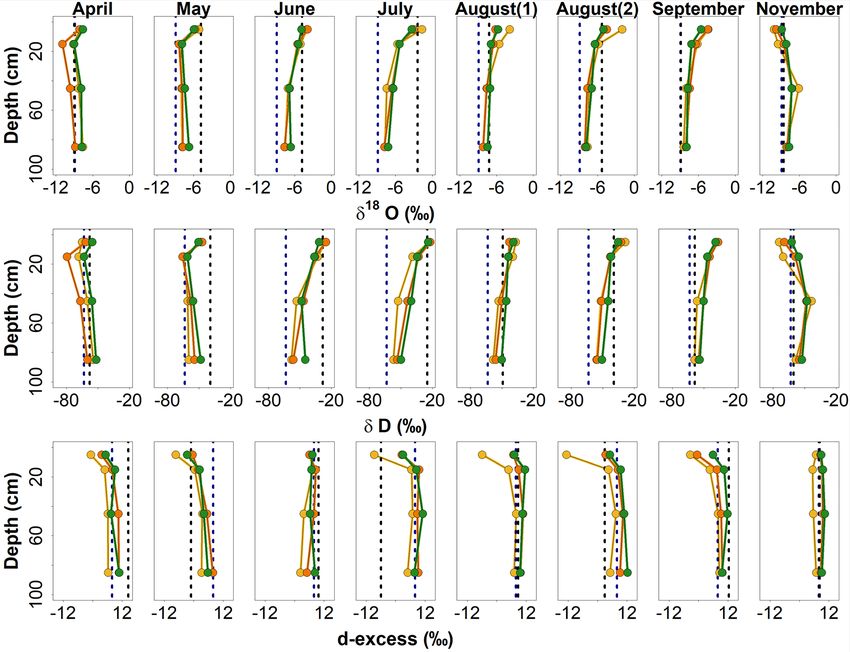
928                  L.-M. Kuhlemann et al.: Using soil water isotopes to infer water partitioning in urban green spaces

temperate regions, the maintenance of urban green spaces           warming and changing precipitation patterns (Nouri et al.,
has so far not required such extensive irrigation. However,        2013, 2016; Pataki et al., 2011b; Vico et al., 2014; Zipper et
an increasing number of exceptionally warm and dry sum-            al., 2017).
mers in recent years has strongly impacted less drought-              A useful tool to disentangle water fluxes and constrain
adapted ecosystems in central and northern Europe (Buras           flow paths in complex landscapes is the application of
et al., 2020), and, consequently, the need for irrigation of ur-   isotopic tracers. Stable isotopes in water behave conser-
ban green spaces may increase in temperate regions in the          vatively and can provide valuable insights into water cy-
future. Therefore, understanding how urban vegetation uses         cling at various spatio-temporal scales (e.g. Clark and Fritz,
and partitions water is crucial for implementing and adapt-        1997; Kendall and McDonnell, 1998). In recent years, they
ing future urban water management and irrigation strategies        have increasingly been applied to understand water parti-
to these conditions.                                               tioning at the soil–plant–atmosphere interface (Sprenger et
    Studying water cycling in urban areas is often challeng-       al., 2016, 2019b), particularly the effects of seasonality and
ing. The urban water cycle is highly complex and comprises         different soil and vegetation types (e.g. Geris et al., 2015;
natural and engineered system components that alter the par-       Sprenger et al., 2017; Oerter and Bowen, 2019). In drought-
titioning and routing of precipitation (Gessner et al., 2014;      sensitive rural areas near Berlin in northern Germany, field-
McGrane, 2016). The spatial distribution of contrasting ur-        based isotope and hydroclimatic measurements (Kleine et al.,
ban land cover with surfaces of different permeabilities forms     2020) and integration of tracer data into process-based mod-
a highly heterogeneous mosaic that impacts infiltration and        els (Douinot et al., 2019; Smith et al., 2020) revealed higher
subsurface flow paths (Fletcher et al., 2013; Pataki et al.,       ET losses and lower groundwater recharge under forest than
2011a; Schirmer et al., 2013). Urban soils are often com-          grassland cover. However, comparable studies are scarce in
pacted and disturbed by the preferential routing of subsurface     urban areas, where the application of isotope tracers remains
infrastructure (pipes, cables, etc.) and contain construction-     a major research frontier (Ehleringer et al., 2016). One of the
based fill materials and rubble (Endreny, 2005). Additionally,     first studies using isotopes in urban green spaces suggested
vegetation types of different heights, microclimates and wa-       groundwater and irrigation as water sources for trees in Los
ter requirements are often heterogeneously distributed across      Angeles (Bijoor et al., 2011). Others found that trees in the
these complex, anthropogenically altered landscapes (Nouri         Salt Lake Valley utilized irrigation water during the growing
et al., 2013). Consequently, the ecohydrological function of       season, though contributions of preceding winter precipita-
urban green spaces likely differs from more natural vegeta-        tion could always be detected (Gómez-Navarro et al., 2019).
tion (McGrane, 2016; Pataki et al., 2011b), and process un-        Oerter and Bowen (2017) used in situ isotope measurements
derstanding from rural areas may not be transferable (Vico         in irrigated urban soils in Utah and observed partitioning of
et al., 2014). For example, urban forests are often a mix of       soil water into mobile and immobile “pools”. While these
native and non-native species (Pataki et al., 2011b) and regu-     studies demonstrate the potential of isotope tracers in urban
larly have to adapt to harsh environments with limited water       applications, there remains a need to address research gaps
availability where surface sealing is extensive (Bijoor et al.,    in understanding water partitioning, not only by irrigated ur-
2011; Vico et al., 2014) and a modified radiation and thermal      ban trees, but also under the complex mosaic of more natural
regime from shading by tall buildings (Asawa et al., 2017).        vegetation types distributed across urban landscapes.
Impervious cover, artificial irrigation and the UHI can extend        To address this, we undertook a study in Berlin, Ger-
the length of the growing season (Zipper et al., 2016) and in-     many, a city characterized by a high cover of urban green
crease urban plant water requirements, thereby posing a risk       and blue spaces, with ∼ 20 % of forest/public green space
for dry-season water stress (Zipper et al., 2017).                 and 7 % surface waters (SenUVK, 2019a). Berlin’s water
    Though recent studies have contributed to an improved          demand is met by local resources (Limberg, 2007; Möller
understanding of urban ecohydrology, there are still consid-       and Burgschweiger, 2008), and climate projections indicate
erable knowledge gaps. Especially quantifying more natural         warmer and drier conditions within the next century, ac-
processes contributing to urban water partitioning remains         companied by an increasing UHI (Langendijk et al., 2019).
challenging (Pataki et al., 2011a). This includes the need         Therefore, improved knowledge of urban water partitioning
for better quantification of ET from contrasting urban veg-        is essential to optimize future benefits from the city’s wa-
etation communities (Pataki et al., 2011a, b; Nouri et al.,        ter resources and adapt to more integrated land and water
2013) and a better understanding of urbanization impacts           management strategies. Our work focused on plot-scale re-
on spatio-temporal variations in infiltration, subsurface flow     search at an ecohydrological observatory in Berlin-Steglitz,
paths and groundwater recharge (Schirmer et al., 2013; Mc-         which provides examples of non-irrigated main functional
Grane, 2016; Pataki et al., 2011a). Quantifying these impacts      urban vegetation types (grassland, shrub and trees) and an
to sustainably manage urban vegetation types and their dis-        opportunity to assess how they affect ecohydrological parti-
tribution and placement in the surrounding environment will        tioning. Our specific objectives are to monitor these differ-
be crucial for adapting urban water management to meet             ent urban soil-vegetation units by (i) quantitatively assessing
the water demand of green spaces during projected climate          ecohydrological partitioning through hydrometric and hydro-

Hydrol. Earth Syst. Sci., 25, 927–943, 2021                                          https://doi.org/10.5194/hess-25-927-2021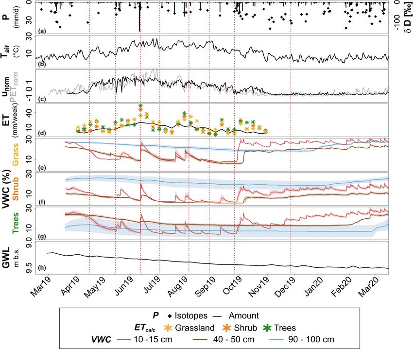
L.-M. Kuhlemann et al.: Using soil water isotopes to infer water partitioning in urban green spaces                                   929

Table 1. Main plant species covering the three sampling plots and their approximate heights and estimated mean leaf area index (LAI) ranges
over the study period in the different vegetation plots.

               Site         Vegetation cover                                                     Vegetation      Estimated
                                                                                                 height               LAI
                            Arrhenatherum elatius
               Grassland                                                                         < 0.5 m                2–3
                            Moss
                            Leaf litter
                                                                                                 < 0.5 m
                            Clematis, Hedera helix
               Shrub                                                                                                    2–4
                            Rubus armeniacus                                                     0.5 to 1 m
                            Young trees (Acer platanoides, Acer pseudoplatanus)                  2 to 3 m
                            Leaf litter
                                                                                                 < 0.5 m
                            Hedera helix, Allium ursinum
                            Various tree species of more than 100 years of age (including oak,
               Trees                                                                             10 to > 20 m           3–5
                            birch, plane, maple, elm, pine, chestnut, ash, lime tree, larch)
                            Some shrub and smaller trees (Prunus padus, Sambucus nigra,
                            Euonymus europaeus, Symphoricarpos, Ligustrum vulgare,               0.5 to 1.5 m
                            Anemone nemorosa, Mahonia)

climatic measurements, (ii) determining the isotopic compo-             the German Weather Service (DWD) is 525–602 mm and
sition of precipitation and soil water to trace ecohydrological         long-term mean annual air temperature 9.3–10.2 ◦ C (DWD,
partitioning effects, (iii) inferring water ages and travel times       2020b). Berlin’s land use includes 34 % sealed urban sur-
of water in the unsaturated zone and (iv) discussing wider              faces (SenStadtWoh, 2017) but also extensive urban green
implications for the upscaling of these findings.                       spaces, including forests (18.1 %), public parks (12.2 %) and
                                                                        agricultural areas (4.2 %; SenUVK, 2019a). Berlin has a high
                                                                        coverage of surface water bodies (Gerstengarbe et al., 2003),
2   Study site                                                          accounting for ∼ 7 % of the city area (SenUVK, 2019a).
                                                                           The Steglitz urban ecohydrological observatory (SUEO) is
Germany’s capital Berlin covers 891 km2 , with a population             located on the Teltow plateau, in the SW of the city (Fig. 1).
of 3.64 million (Amt für Statistik Berlin-Brandenburg, 2020;            The surrounding district is covered by residential areas and
Fig. 1). Located within the Northern European Plain, Berlin’s           roads (55 %), forest (24 %), water bodies (11 %) and public
flat topography was formed during the Pleistocene glaciation            green space (9 %; SenUVK, 2019b). The SUEO itself com-
and primarily consists of Quaternary deposits of unconsol-              prises a ∼ 8000 m2 large research garden. The elevation is ∼
idated sediments (Stackebrandt and Manhenke, 2010). The                 45 m a.s.l. (SenStadt, 2010b), and groundwater levels are 10–
NE–SW-trending sand and gravel deposits of the Berlin–                  15 m below surface (m b.s.; SenStadt, 2010a). Buildings and
Warsaw glacial spillway are surrounded by the elevated                  some older trees were established > 100 years ago, though
plateaus of Barnim and Teltow in the north and south, cov-              the current garden dates to the 1950s when the Technical
ered by subglacial till (Limberg and Thierbach, 1997; Lim-              University (TU) Berlin started using the site (Bornkamm
berg, 2007). Groundwater flow in Berlin’s ∼ 150 m thick                 and Köhler, 1987). Recently, further adjustments to the land
freshwater aquifer of Tertiary–Holocene age (Limberg and                cover have been made through management of the research
Thierbach, 1997) is directed from the plateaus towards the              garden and installation of a 40 m eddy flux tower as part
rivers Spree and Havel in the glacial valley (velocities ∼ 10–          of the Urban Climate Observatory (UCO) of the TU Chair
500 m/yr; Limberg, 2007). Berlin meets its water demand                 of Climatology for long-term observations of atmospheric
through a semi-closed water cycle, whereby groundwater                  processes in cities (Fig. 1). The premises are now covered
is abstracted from local storage and bank filtration, while             by buildings (∼ 17 %); different types of non-irrigated urban
treated sewage water is discharged back into the surface wa-            green spaces, including grassland (∼ 16 %), shrub (∼ 7 %)
ters (Limberg and Thierbach, 1997; Limberg, 2007; Möller                and trees (∼ 39 %); and semi-permeable or sealed pathways
and Burgschweiger, 2008).                                               and parking spaces (∼ 16 %). Soils can be characterized as
   Recharge is low due to high area-weighted ET of                      medium silty and loamy sands (SenStadtWoh, 2018). They
367 mm/yr (60 % of precipitation), plus 152 mm/yr evapo-                reflect anthropogenic impacts, as the naturally occurring sub-
ration from surface waters (SenStadtWoh, 2019). Long-term               glacial till is covered by 50–180 cm of debris, sandy materi-
mean annual rainfall (1981–2010) from weather stations of

https://doi.org/10.5194/hess-25-927-2021                                                 Hydrol. Earth Syst. Sci., 25, 927–943, 2021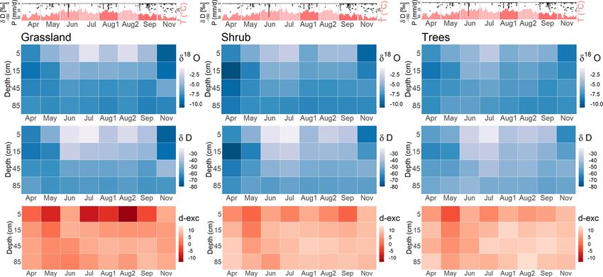
930 L.-M. Kuhlemann et al.: Using soil water isotopes to infer water partitioning in urban green spaces
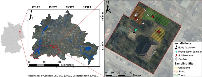
Figure 1. Location of Berlin within Germany (left); location of the district of Steglitz-Zehlendorf and the SUEO (red) with Berlin’s surface
waters in blue (middle); and the SUEO (right) with vegetation plots and installations of soil moisture and sap flow measurements, precipitation
sampler and eddy flux tower.
als and a humus layer from long-term intensive cultivation Table 2. Characteristics of trees and sensors of the sap flow instal-
and gardening (Bornkamm and Köhler, 1987). lation.
Tree species Diameter Number Sensor
3 Methods and data at breast of type
height (cm) sensors
Monitoring was carried out from March 2019 to March 2020, Maple (Acer platanoides, 8.9 2 TDP10
with particular focus on the growing season (April to Oc- Acer pseudoplatanus) 10.5 2 TDP30
tober). Climate data were available from Berlin-Dahlem, 14.0 2 TDP30
∼ 1500 m west of the site (precipitation (P ), air tempera-
Elm (Ulmus glabra) 18.5 2 TDP30
ture (Tair ), relative humidity (RH), vapour pressure; DWD,
Plane (Platanus x hybrida) 111.4 4 TDP30
2020a) and the TU UCO eddy flux tower (radiation fluxes, Oak (Quercus robur) 67.8 4 TDP50
wind speed, ET estimates; Fig. 1). Groundwater-level data
were available from the Berlin Senate (SenUVK, 2020).
Three generic urban vegetation types (grassland, shrub and
trees) were selected as representative urban soil-vegetation 1.5 cm of paraffin oil was added to each bottle, and occa-
plots (Fig. 1). Each plot was characterized by species typi- sional samples of < 1.5 mm were rejected in case of ex-
cally found in more natural urban green spaces (e.g. parks; aggerated fractionation effects. For soil water isotope sam-
Table 1). The plots received no irrigation water throughout pling, eight monthly campaigns were conducted from April–
the study period. For soil moisture monitoring, CS650 re- November 2019. In each campaign, samples were taken un-
flectometers (Campbell Scientific, Inc.; accuracy ±3 % for der grassland, shrubs and trees (Fig. 1). To cover potential
volumetric water content, VWC) were installed at 10–15 cm heterogeneities at the site, three spatially distributed points
(VWC12.5 ), 40–50 cm (VWC45 ) and 90–100 cm (VWC95 ) in were sampled respectively under each vegetation type. Du-
representative locations within each plot (Fig. 1), with dupli- plicate soil cores were taken at 0–10, 10–20, 40–50 and 80–
cate sensors at each depth. Sensors were connected to CR300 90 cm depth at each location using a soil auger. Samples of
data loggers in ENC8/10 enclosures (Campbell Scientific, ∼ 250 cm3 volume were filled into bags (WEBAbag, Silver
Inc., Logan, USA). For sap flow, a FLGS-TDP XM1000 Range, Weber Packaging, Germany), immediately sealed,
sap velocity logger system (Dynamax Inc, Houston, USA) avoiding air inclusions, and stored in a thermally isolated
measuring temperature differences between heated sensors box. Groundwater was sampled seasonally for isotope anal-
(Granier, 1987) was installed at 1.5 m height within six rep- ysis from October 2018 to July 2019 across the whole city
resentative urban trees (Fig. 1, Table 2). Dependent on tree (Kuhlemann et al., 2020a), including an observation well
height and age, two or four sets of sensors were installed in ∼ 2.5 km NE of the site, which was used in comparison to
each cardinal direction, with more in older, larger trees. P the SUEO samples for context.
was sampled daily for isotope analysis using a 3700 sam- Filtered P , groundwater and surface water samples were
pler (Teledyne Isco, Lincoln, USA). To prevent evaporation, analysed by cavity ring-down spectroscopy with an L2130-i
Hydrol. Earth Syst. Sci., 25, 927–943, 2021 https://doi.org/10.5194/hess-25-927-2021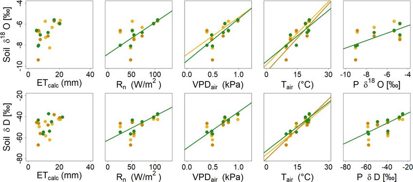
L.-M. Kuhlemann et al.: Using soil water isotopes to infer water partitioning in urban green spaces                           931

isotopic water analyser (Picarro, Inc., USA). Four lab stan-      From daily P isotopes, a local meteoric water line (LMWL)
dards were used for linear correction and standards of the        was calculated by amount-weighted least square regression
International Atomic Energy Agency (IAEA) for calibration.        (Hughes and Crawford, 2012). For all isotope samples, deu-
Results were expressed in δ notation with Vienna Standard         terium (d-) excess was calculated as d-exc = δD − 8 · δ 18 O
Mean Ocean Water (VSMOW). Mean analytical precision               (Dansgaard, 1964). To compare soil isotope data with depth,
was 0.05 ‰ standard deviation (SD) for δ 18 O and 0.16 ‰          geometric means were calculated from plot and depth repli-
SD for δD.                                                        cates. Mean values for soil profiles at the individual sites
    Soil samples were analysed using the direct equilibrium       and sampling campaigns were compared to mean ETcalc , Tair ,
method (Wassenaar et al., 2008). First, additional bags were      VPDair , Rn and P isotopes in the month before or weeks be-
filled with 10 mL of three liquid lab standards (with dupli-      tween each sampling campaign through linear regression. A
cates). Second, all bags were inflated with dry air, welded,      mean value of seasonally sampled groundwater (Kuhlemann
equipped with a silicon septum and stored for ∼ 48 h to equi-     et al., 2020a) was calculated to compare to P and soil water
librate. Third, the vapour phase was analysed using the Pi-       isotopes.
carro L2130-i by inserting a needle attached to a tube into the      To obtain a first approximation of soil water ages at differ-
bags through the silicon. Standards were measured at the be-      ent sites and depths, stable isotopes of P and soil water were
ginning, middle and end of each run. Criteria for plateau de-     used to calculate fractions of young water (Fyw ) by sine-
tection during analysis were SD H2 O < 100 ppm, SD δ 18 O <       wave fitting of seasonal cycles (von Freyberg et al., 2018).
0.35 ‰ and SD δD < 0.55 ‰. Analytical precision was mean          Strongly fractionated samples from the upper two soil layers
SD of 0.14 ‰ and 0.34 ‰ for δ 18 O and δD, respectively. Se-      were identified by comparing to incoming P and excluded
lected bags were remeasured after 2–4 weeks for gas matrix        from analysis if the soil isotopic values were above the max-
correction (Grahler et al., 2018). Samples were subsequently      imum P isotopic value. Mean transit times (MTTs) were cal-
oven-dried at 105 ◦ C for 24 h and weighted to determine their    culated by a lumped convolution method (McGuire and Mc-
gravimetric water content. Samples with < 3 g of water were       Donnell, 2006). Amount-weighted weekly P isotope means
excluded from analysis (Hendry et al., 2015).                     were used as input with a 1-year spin-up period. Shape (α,
    For sap flow, individual sensor values for each tree were     range 0.001–5) and scale (β, range 1–50) parameters were
averaged, converted to sap flux velocity (u) in millimetres       estimated for a gamma transfer function by maximizing the
per hour (mm/h) (Granier, 1987) and summed up to daily to-        Kling–Gupta efficiency (KGE; Gupta et al., 2009) of esti-
tals. Potential evapotranspiration (PET) was estimated using      mated monthly soil isotopes to the measured monthly soil
the FAO Penman–Monteith method (Allen et al., 1998). For          water isotope data.
a more generalized view on the dynamics during the grow-
ing season, both u and PET were then normalized (to unorm
and PETnorm , respectively) by subtracting the mean over the      4     Results
study period from the individual daily values and dividing by
SD.                                                               4.1    Ecohydrological partitioning of water under
    At each site, VWC of duplicate sensors was averaged                  different generic vegetation communities
hourly. For the growing period, a mass balance approach was
applied for a first approximation of ET. As the site topogra-     Monitoring followed the 2018 summer drought which af-
phy was flat and the study period dry and consistent with the     fected much of central Europe (Buras et al., 2020) and
soil moisture data, we assumed no percolation below 50 cm         below-average P in the winter of 2018/2019. Compared to
and negligible lateral flow. At each site, daily storage change   the long-term mean (1981–2010; DWD, 2020b), 2018 was
was calculated as 1S = VWC12.5 · h12.5 + VWC45 · h45 with         +1.6 ◦ C warmer and had a P deficit of 232 mm (or 39 %) in
h as depth of the soil layer. Daily ET was then estimated         Berlin Dahlem (DWD, 2020a). At the start of the study from
as ETcalc (mm) = 1S − P . Occasional small negative daily         March–May, mean daily Tair was ∼ 10 ◦ C, and P was low,
ETcalc values resulting from P inputs that did not infiltrate     at ∼ 15 mm/month (Fig. 2a, b). From mid-May to mid-June,
to sensors were assumed to be zero. Daily ETcalc was then         Tair increased to ∼ 18 ◦ C, and several heavy convective P
aggregated to weekly sums. The procedure was repeated for         events totalled > 100 mm (Table 3, Fig. 2a, b). Conditions re-
ET from the eddy flux tower at 30 m height. For compari-          mained warm and dry until late September, with most P oc-
son of accumulated ET, monthly ETcalc at the individual sites     curring in further high-intensity convective events (Table 3,
was summed over the growing period, and a weighted mean           Fig. 2a, b). The remaining period until March 2020 was char-
was calculated considering the fractional distribution of veg-    acterized by lower Tair and more frequent, low-intensity P .
etation types at the site. Weekly means were computed for         Overall, 2019, similar to 2018, was warmer and drier than
environmental variables (VWC12.5 ; vapour pressure deficit        the long-term average, with a P deficit of 85 mm (14 %) and
(VPDair ) calculated from Tair and RH; and net radiation (Rn )    Tair + 1.7 ◦ C (DWD, 2020a, b).
calculated from short- and longwave fluxes in 2 m height)            Variable Tair and P during the study period inevitably
to explore linear correlation with weekly ETcalc and unorm .      impacted soil water storage. Under grassland, VWC12.5 de-

https://doi.org/10.5194/hess-25-927-2021                                          Hydrol. Earth Syst. Sci., 25, 927–943, 2021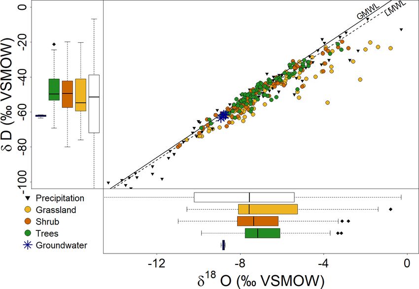
932                   L.-M. Kuhlemann et al.: Using soil water isotopes to infer water partitioning in urban green spaces

Table 3. Climate parameters (DWD, 2020a) and VWC under the different vegetation units in the month before or weeks between the
individual soil sampling campaigns.

 Sampling                       1 (Apr)     2 (May)      3 (Jun)     4 (Jul)   5 (Aug1)     6 (Aug2)         7 (Sep)          8 (Nov)
 Time period                 16 March–     16 April–   15 May–     12 June–      3 July–      5–28       28 August–    25 September–
                               16 April      15 May     12 June       3 July   5 August      August    25 November      27 November
                    Mean           8.12       11.70       17.96       21.50       19.35        20.09           17.65              9.25
 Tair (◦ C)
                    SD             3.12        3.13        4.13        3.31        3.28         2.46            4.00              4.22
 P (mm)             Sum           11.90       13.20      103.10        2.80       63.70        19.40           41.80           121.20
                    Mean          24.30       18.34       16.50       19.16       15.35        14.46           12.98             20.28
 VWC grassland
                    SD             1.27        1.38        1.56        2.51        1.62         1.27            1.60              2.37
                    Mean          16.41       13.89       12.90       12.33         9.24        8.51            8.27             12.20
 VWC shrub
                    SD             0.55        0.74        1.58        2.21         0.61        0.37            0.45              1.19
                    Mean          20.14       15.30       12.57       11.74         9.78        9.12            8.98             11.71
 VWC trees
                    SD             0.50        1.80        1.64        1.95         0.91        0.40            0.55              1.18

Figure 2. (a) Daily P sums (DWD, 2020a) and isotopic composition, (b) mean daily Tair (DWD, 2020a), (c) daily unorm and PETnorm (grey)
(d) weekly ETcalc and ET of the eddy flux tower (grey line), (e–g) soil VWC at different depths and sites and (h) mean weekly groundwater
level (GWL) near the SUEO (SenUVK, 2020). Dashed red lines mark the days on which soil samples were taken for monthly soil water
isotope analysis.

Hydrol. Earth Syst. Sci., 25, 927–943, 2021                                                https://doi.org/10.5194/hess-25-927-2021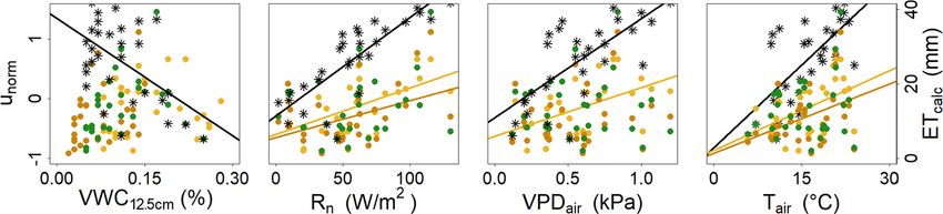
L.-M. Kuhlemann et al.: Using soil water isotopes to infer water partitioning in urban green spaces                                      933

Figure 3. Linear correlation of hydroclimatic variables (VWC12.5 , Rn , VPDair , Tair ) with measured weekly unorm at the tree site (asterisk)
and calculated weekly ETcalc at the grassland (yellow), shrub (orange) and tree (green) sites.

Table 4. Accumulated ETcalc over the growing period of 2019.             P events. From August–October, variability remained, but
                                                                         unorm decreased, with short-term decreases around P events.
                                  ETcalc (mm)                            After slight variability in October, rates permanently de-
                         Grassland      Shrub      Trees                 creased after leaf fall. PETnorm (Fig. 2c) showed similar sea-
                                                                         sonality, with the highest rates in June–July. However, dur-
           April             62.00      33.82     51.76                  ing some of the highest PETnorm increases, unorm did not re-
           May              112.81      80.18    116.25                  spond.
           June             209.16     171.21    203.51                     Weekly ETcalc ranged from < 5 mm/week under dry, cool
           July             262.58     216.60    244.16
                                                                         conditions to ∼ 40 mm/week after heavy P events (Fig. 2d).
           August           335.26     261.36    305.78
           September        364.32     288.11    345.08
                                                                         At the start of the growing period in April, ETcalc was high-
           October          413.60     343.92    415.59                  est in grassland, but after leaf-out, the tree site was higher
                                                                         for some weeks in May and June. Increases in ETcalc after
                                                                         large P events were especially pronounced at the tree site,
                                                                         while grassland ETcalc remained highest during dry periods
creased to < 10 % during summer, with transient increases                in July and August (Fig. 2d). Shrub patterns were variable,
after P (Fig. 2e). Prolonged re-wetting in October returned              with ETcalc lowest at the start of the growing season and from
VWC12.5 to March 2019 levels, with minor variability there-              July to October but intermediate from May to July and Oc-
after. At the other sites (Fig. 2f, g), VWC12.5 was lower gen-           tober and in response to P events (Fig. 2d). Accumulated
erally, decreasing during dry periods to ∼ 2 % in June/July              ETcalc by October was similar (∼ 415 mm) at the grassland
(shrub) and ∼ 4 % in September (trees). Wetness increased                and tree sites but lower at the shrub site (344 mm; Table 4).
again over the winter. At all sites, VWC12.5 of duplicate                ETcalc variations roughly resembled the dynamics measured
sensors was in a similar range. VWC45 dynamics were                      by the eddy flux tower, although those were more damped
“damped” in comparison. Under grassland, VWC45 declined                  (Fig. 2d) and totaled only 285 mm over the same time pe-
over summer to < 10 % from May onwards, until increas-                   riod. Area-weighted summertime (May–October) ETcalc for
ing again a few days later than the shallower soil in October            the vegetation community was 351 mm.
(Fig. 2e). Under shrub, patterns were similar (Fig. 2f). Un-                The highest correlations with environmental variables
der trees, VWC45 slowly declined to ∼ 15 % throughout the                (Fig. 3, Table 5) were observed between unorm and Rn
summer, with no marked response to any P . It only started               and less strongly between unorm and VWC12.5 , VPDair and
to increase again in February 2020 (Fig. 2g). Temporal vari-             Tair . Correlation between unorm and VWC12.5 was negative,
ations in VWC95 were lowest. Values continuously declined                while all others were positive. Significant positive correla-
over summer, with no response to P . Under grassland and                 tions were also observed between grassland ETcalc and Rn ,
shrub, VWC95 was higher than at shallower depths for most                VPDair and Tair . Correlations with ETcalc at the shrub and
of the growing period (Fig. 2e, f). Under trees, VWC95 was               tree sites were low.
lower, with a high discrepancy between duplicate sensors
(Fig. 2g). VWC95 only started to increase again in January
                                                                         4.2    Ecohydrological partitioning under different urban
(grassland, shrub) and March 2020 (trees). Despite some
                                                                                soil-vegetation units inferred from the isotopic
variation, the groundwater level in the closest well (500 m
                                                                                composition of precipitation and soil water
SE of the SUEO) continuously declined from 9.2 to 9.5 m b.s.
(Fig. 2h), suggesting no net recharge during the study period.
   Daily unorm (Fig. 2c) showed a marked increase follow-                P isotopes were generally depleted in winter and more en-
ing the start of the growing season in April 2019 as trees               riched in summer. The range was −17.3 ‰ to −0.3 ‰ for
came into leave. Values were highest from May–July, with                 δ 18 O, −131.3 ‰ to −12.7 ‰ for δD and −10.4 ‰ to 15.7 ‰
daily variability and negative troughs coinciding with larger            for d-excess (Fig. 2a). The amount-weighted LMWL during

https://doi.org/10.5194/hess-25-927-2021                                                  Hydrol. Earth Syst. Sci., 25, 927–943, 2021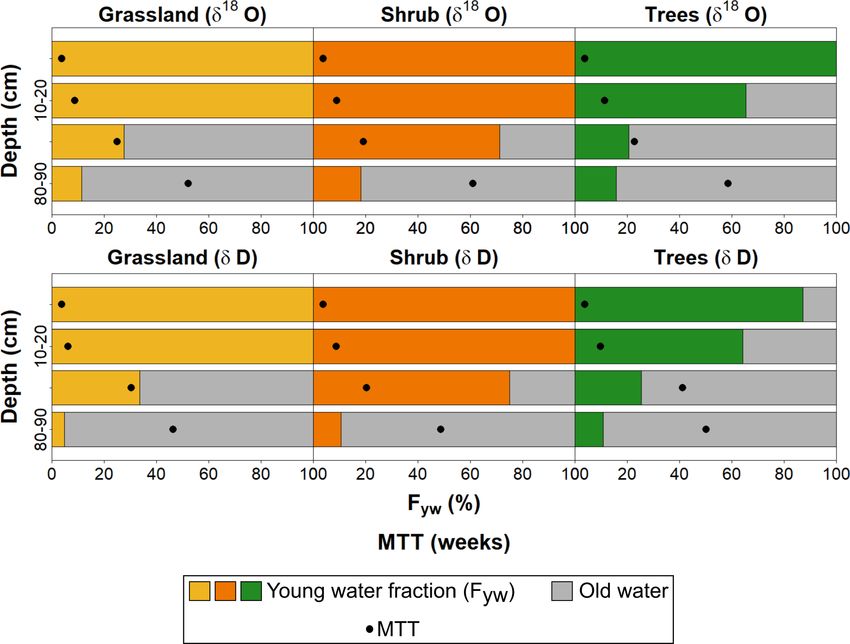
934                    L.-M. Kuhlemann et al.: Using soil water isotopes to infer water partitioning in urban green spaces

Table 5. R 2 and p values of the parameters used for the correlation plots of unorm and ETcalc (Fig. 3).

                                      VWC12.5                   Tair                       VPDair                        Rn
                                 R2         p value      R2            p value             R2          p value    R2          p value
        unorm                  0.27    3.00 × 10⁻³     0.44    4.56 × 10⁻⁵               0.49     1.33 × 10⁻⁵    0.71   2.49 × 10⁻⁹
                  Grassland    0.01             0.54   0.25    4.06 × 10⁻³                0.29    1.70 × 10⁻³    0.39   1.70 × 10⁻⁴
        ETcalc    Shrub        0.10             0.08   0.16            0.03               0.05            0.23   0.20           0.01
                  Trees        0.10             0.08   0.05            0.24      1.00 × 10 − 3            0.86   0.09           0.10

                                                                           values were depleted, especially under shrub. Values resem-
                                                                           bled the isotopic signal of incoming P at 0–10 cm, while
                                                                           values at 10–20 cm were even more depleted (Figs. 5, 6).
                                                                           D-excess was more negative at the grassland site, coincid-
                                                                           ing with higher ETcalc (Fig. 2d). Following little P and in-
                                                                           creasing Tair and unorm , VWC had decreased by May (Fig. 2),
                                                                           and soil water became more enriched, especially at 0–10 cm,
                                                                           while d-excess decreased throughout the profile, especially
                                                                           under grassland (Figs. 5, 6). While Tair and unorm remained
                                                                           high over summer, the large convective P event preceding
                                                                           the June sampling led to higher VWC and ETcalc , especially
                                                                           at the tree site (Fig. 2), and a more enriched isotopic compo-
                                                                           sition at 0–20 cm. D-excess, however, became more positive
                                                                           in the shallow soil at all sites, overprinting previous signals
                                                                           of fractionation and displacing waters with lower d-excess to
Figure 4. Dual isotope and box plots showing the isotopic composi-         depth (Figs. 5, 6).
tion of incoming P and local groundwater sampled ∼ 2.5 km north               Through the warm, dry July–September period, VWC re-
of the SUEO (Kuhlemann et al., 2020a), as well as the isotopic com-        mained low (Fig. 2), and the isotopic composition of the shal-
position of sampled bulk soil water at different depths between 0          low soil remained enriched but became depleted with depth
and 90 cm under grassland, shrub and tree sites.
                                                                           (Figs. 5, 6). D-excess in the shallow soil was strongly neg-
                                                                           ative at the grassland (Figs. 5, 6), where ETcalc was slightly
                                                                           higher (Fig. 2d). P events in August temporarily increased
our sampling period (Fig. 4) was δD = 7.82 ± 0.26 · δ 18 O +               VWC (Fig. 2e–g) and slightly moderated the fractionation
6.31 ± 1.25 (R 2 = 0.974).                                                 effects (Figs. 5, 6). Importantly, it is notable from Fig. 6 that
   Soil water samples under grassland showed the widest                    from April to July, the isotopic signature of the shallow soil
range for δ 18 O, and some surface layer samples deviated sub-             (0–10 cm) always moved in the direction of incoming P in
stantially from the global meteoric water line (GMWL) and                  the weeks preceding the respective samplings. From August
LMWL (Fig. 4). However, across the entire soil profile (0–                 to September, however, the isotopic composition of the shal-
90 cm), isotopes were least variable and more enriched under               low soil became increasingly more enriched than the incom-
trees. Local groundwater was generally more depleted, while                ing P , especially under grassland (Fig. 6). After Tair , unorm
most soil water samples were more enriched and plotted fur-                and ETcalc decreased and more frequent P started in Oc-
ther up the GMWL and LMWL.                                                 tober (Fig. 2), soil water isotopes in November were more
   Soil water isotopic composition generally became more                   depleted. However, the deeper soil, especially at 40–50 cm,
depleted with depth (Table 6). Shallow soil layers under                   remained more enriched (Figs. 5, 6). Correlations between
grassland were more enriched compared to shrub and trees,                  mean monthly δ 18 O and δD of the soil profiles and selected
while the deeper soil layers were most enriched beneath                    environmental variables in the month before or weeks be-
trees. Mean negative d-excess, indicating evaporative losses               tween the samplings are shown in Fig. 7 and Table 7. Under
(Dansgaard, 1964), was observed in the upper soil under                    grassland, soil isotopes showed a strong positive correlation
grassland (Table 6), where Rn and Tair significantly influ-                with Tair and a weaker one with VPDair . Under trees, soil
enced the ET rates (Fig. 3, Table 5), but not under shrub and              isotopes showed significant positive correlations with Rn ,
trees, where d-excess remained positive.                                   VPDair , Tair and incoming P isotopes. Under shrub, corre-
   Soil water isotopes also showed strong temporal variation.              lations were weaker; only a positive correlation with Tair was
In mid-April, when P was low but the soils still wet (Fig. 2),             evident.

Hydrol. Earth Syst. Sci., 25, 927–943, 2021                                                     https://doi.org/10.5194/hess-25-927-2021
L.-M. Kuhlemann et al.: Using soil water isotopes to infer water partitioning in urban green spaces 935 Figure 5. Heat maps showing the isotopic composition of the different soil layers during the monthly sampling campaigns (for abbreviations, see Table 3) in ‰ VSMOW. Climate parameters (top; DWD, 2020a) mark the daily Tair and P during the sampling period. Figure 6. Isotopic depth profiles showing geometric means at different depths at the grassland (yellow), shrub (orange) and tree sites (green) during the monthly sampling campaigns. Dashed lines marking the mean isotopic composition of groundwater (blue) and weighted P mean in the month before or weeks between the sampling campaigns are given for reference. https://doi.org/10.5194/hess-25-927-2021 Hydrol. Earth Syst. Sci., 25, 927–943, 2021
936                    L.-M. Kuhlemann et al.: Using soil water isotopes to infer water partitioning in urban green spaces

Table 6. Number of samples (n) with measured isotopic composition of P and soil water under the three soil-vegetation units for different
sampling depths.

                                                              Precipitation
                                                        δ 18 O (‰)   δD (‰)      d-exc. (‰)
                                               n              78         78             78
                                               Mean        −8.23     −58.74           7.06
                                               SD           3.58      27.65           5.21

                                                                Soil water
                               Grassland                              Shrub                                   Trees
                  δ 18 O (‰)   δD (‰)      d-exc. (‰)   δ 18 O (‰)   δD (‰)      d-exc. (‰)     δ 18 O (‰)   δD (‰)   d-exc. (‰)
        0–10 cm
        n                        23                                    22                                      23
        Mean         −5.01     −42.83          −2.69       −5.70     −41.61           4.59         −6.00     −43.07        5.54
        SD            2.83      18.57           7.57        2.21      16.22           5.03          1.69      12.50        3.69
        10–20 cm
        n                        23                                    22                                      23
        Mean         −6.92     −50.53           6.14       −7.16     −49.50           9.29         −7.26     −49.74        9.79
        SD            1.74      14.75           3.39        1.72      14.76           3.22          1.21      10.18        3.33
        40–50 cm
        n                        22                                    17                                      22
        Mean         −7.34     −53.90           6.47       −7.50     −51.22          11.02         −7.18     −48.52       10.37
        SD            1.33       6.69           8.25        1.04       8.36           2.91          0.72       7.00        3.68
        80–90 cm
        n                        18                                    14                                      18
        Mean         −7.72     −57.65           5.69       −8.03     −55.96          10.97         −7.12     −48.06        9.63
        SD            1.03       2.28           8.60        0.60       3.94           3.00          1.13       7.93        2.52

4.3   Water ages and travel times of water in the                      KGE fit 0.44–0.62) and trees (21 to 40 weeks, KGE fit 0.62–
      unsaturated zone under different urban vegetation                0.80). In 80–90 cm, Fyw was low, especially under grassland
      units                                                            (5 %–11 %; Fig. 8) where VWC95 was higher (Fig. 2e), but
                                                                       also at the drier shrub and tree sites (11 %–18 %). MTTs were
Estimated Fyw values of soil water at the different sites and          substantially longer than at shallower depths, especially un-
depths indicate that under grassland, where isotopes and d-            der trees (50–59 weeks) and shrub (49–62 weeks). Due to
excess suggested highest evaporative losses over the summer            the lack of variability and the limited observation period, es-
(Figs. 5, 6), the shallow soil was dominated by young wa-              timates at depth were more uncertain, with a KGE fit of 0.13–
ter < 8 weeks old (Fig. 8). MTTs were < 6 weeks in the                 0.54 at all sites.
upper 20 cm, with a good KGE fit (0.39–0.93; Fig. 8). A
similar pattern was estimated for shrub. Under trees, where
VWC12.5 was low (Fig. 2g) and isotopes indicated less pro-
nounced evaporative enrichment (Figs. 5, 6), older water con-          5      Discussion
tributed ∼ 35 % in 10–20 cm depth. MTTs of < 8.3 weeks
(KGE fit 0.71–0.94) in the upper 20 cm were slightly higher            5.1     Quantitative assessment of ecohydrological
than under grassland and shrub. In the mid-profile at 40–                      partitioning under different urban soil-vegetation
50 cm depth, Fyw remained high (> 70 %) under shrub,                           units
where VWC45 was lowest (Fig. 2f), while only 20 %–33 %
of young water could be observed under grassland and trees             Through our integrated plot-scale study during and after the
(Fig. 8). Similarly, MTTs were lower under shrub (17–18                exceptional summers of 2018 and 2019, we gained novel
weeks, KGE fit ∼ 0.81) than under grassland (23–29 weeks,              insights into ecohydrological partitioning in urban green

Hydrol. Earth Syst. Sci., 25, 927–943, 2021                                                   https://doi.org/10.5194/hess-25-927-2021
L.-M. Kuhlemann et al.: Using soil water isotopes to infer water partitioning in urban green spaces 937
Figure 7. Linear correlations at the grassland (yellow), shrub (orange) and tree sites (green) between mean analysed soil water isotopic
composition on the individual sampling dates and mean values of environmental parameters in the month before or weeks between the
respective samplings.
Table 7. Correlations between analysed soil water isotopic composition and mean environmental variables ∼ 4 weeks prior to the sampling
(Fig. 7).
ETcalc Tair VPDair Rn P isotopes
R2 p value R2 p value R2 p value R2 p value R2 p value
Grassland 0.15 0.38 0.93 5 × 10⁻⁴ 0.60 0.04 0.32 0.18 0.44 0.10
δ 18 O Shrub 0.35 0.16 0.65 0.03 0.35 0.16 0.28 0.22 0.45 0.10
Trees 0.26 0.24 0.62 0.04 0.79 7 × 10⁻³ 0.81 6 × 10⁻³ 0.85 4 × 10⁻³
Grassland 0.19 0.32 0.91 8 × 10⁻⁴ 0.54 0.06 0.33 0.17 0.38 0.14
δD Shrub 0.38 0.14 0.78 8 × 10⁻³ 0.44 0.10 0.31 0.19 0.44 0.11
Trees 0.17 0.37 0.85 3 × 10⁻³ 0.89 1 × 10⁻³ 0.72 0.02 0.68 0.02
spaces under dry, warm conditions which will likely become serving water resulting from moisture stress from the dry
more common in future. subsoil. This may at least in part also explain the ET losses
Firstly, by combining sap flow measurements with soil under trees being less than the grassland, if low soil moisture
moisture and climate data, we were able to gain some first in- limits ET. This may also be the result of “memory effects”,
sights into the response of non-irrigated urban trees to these i.e. the depletion of soil storage, after the extreme drying in
conditions. The observed dependence of seasonal unorm (as summer 2018 and lower than average re-wetting in the fol-
a proxy for transpiration) on Rn , VPDair and Tair is in agree- lowing winter. In addition, the delivery of rainfall in intense
ment with previous observations in urban trees that showed convectional events may limit the time the canopy is wet,
temporal sap flux variability is largely driven by variations in with low radiation and high humidity at such times limit-
vapour pressure deficit and photosynthetically active radia- ing interception losses compared to more upland, windy sites
tion (Asawa et al., 2017; Pataki et al., 2011b). Though some (e.g. Soulsby et al., 2017). By selecting a mixed urban tree
larger P events temporarily increased VWC, the simultane- assemblage of different tree ages and species, our approach
ous increase in RH and decrease in Rn and VPDair caused the likely captures the heterogeneity in urban green spaces (cf.
transpiration rates to temporarily decrease, explaining nega- Nouri et al., 2013).
tive troughs and correlation. Such low dependency of tran- Secondly, the quantitative assessment of urban ET patterns
spiration rates on soil water content, despite limited P , is in under a mosaic of green spaces, a key challenge in urban eco-
contrast to low-energy headwater catchments (Wang et al., hydrology (e.g. Nouri et al., 2013; Pataki et al., 2011a, b),
2017). This may indicate that transpiration rates at our site showed that “green water” fluxes in the growing period in-
showed a certain resilience against prolonged drought pe- creased in the order shrub < grassland ∼ = trees. These differ-
riods and depletion of soil moisture, which would coincide ences in ecohydrological partitioning under contrasting ur-
with a rural study east of Berlin following the 2018 drought ban vegetation types during the 2019 growing season were
(Kleine et al., 2020). However, decreased unorm during times in some ways counter-intuitive. At the grassland site, shad-
of highest PETnorm would be consistent with the trees con- ing from surrounding trees was limited and the soil was only
https://doi.org/10.5194/hess-25-927-2021 Hydrol. Earth Syst. Sci., 25, 927–943, 2021938 L.-M. Kuhlemann et al.: Using soil water isotopes to infer water partitioning in urban green spaces
water balance may not fully account for spatial heterogene-
ity in soil moisture distribution and have uncertainties in ac-
counting for deep percolation or capillary rise (Nouri et al.,
2013). Nevertheless, the general similarity of ETcalc dynam-
ics to values independently measured by the eddy flux tower
indicates that it provided a reasonable first approximation.
Higher green space ETcalc than the flux tower’s estimates
was expected, as the tower’s 30 m height integrates a wider
footprint of mixed urban (impermeable) surfaces that can in-
crease surface runoff and decrease ET (e.g. Endreny, 2005;
Fletcher et al., 2013; Schirmer et al., 2013).
5.2 Isotopic composition of precipitation and soil water
and its indications for ecohydrological partitioning
under different urban vegetation types
Figure 8. Fyw and MTTs at different sites and depths (0–10 cm, The LMWL of Berlin-Steglitz was close to the LMWLs pre-
10–20 cm, 40–50 cm and 80–90 cm) during the growing period of viously reported for Germany and Berlin (Stumpp et al.,
2019. 2014). The measured soil water isotopic composition largely
supports inference from the hydrometric measurements but
provides more nuanced insights into sources, movement and
covered by the grass sward and patchy moss ground level. mixing of stored waters. Over the growing season, changes
Consequently, with limited interception, incoming P could in soil water isotopes with depth reflected the general pattern
directly infiltrate and drive the rapid soil moisture dynamics of infiltrating P becoming more enriched after evaporative
whilst simultaneously sustaining transpiration. Similarly, the losses in the upper 30 cm of soil, while the fractionation sig-
sparse soil cover enhanced atmospheric exposure for evapo- nal diminishes with depth as infiltrating P mixes with soil
ration at the soil surface when Tair , Rn and VPDair were high. waters, damping seasonal variability (Sprenger et al., 2016).
In contrast, at the tree site, soil was covered by a ground layer The most pronounced isotopic enrichment and negative d-
of ivy and leaf litter and shaded by an almost-closed canopy excess under grassland support a pattern of higher soil evap-
during the growing season. It is likely that much higher in- orative losses.
terception losses and transpiration by trees and the under- In April and May, more depleted values at 10–20 cm depth
storey, the latter reflected by unorm , contributed to higher at all sites would be consistent with stored water from win-
ET rates at this site, leading to drier soils, less responsive- ter P prior to sampling. In contrast, the negative d-excess
ness to P and longer time lags until re-wetting of the deeper in the upper 10 cm already indicates the effect of evapora-
soil in autumn. Inter-sensor variation of VWC95 under trees tive fractionation (Sprenger et al., 2019a). Subsequent in-
likely reflects heterogeneity in subsurface texture, as interca- coming P and soil evaporation, especially at the grassland
lations of sandy and loamy materials were present through- site, strongly influenced the isotopic signal from May to July,
out the site. Over most of the study period, the shrub site though soil water in the upper 10 or even 20 cm was persis-
exhibited intermediate hydrological responses to grassland tently more enriched than incoming P in the second half of
and trees, e.g. regarding VWC and ETcalc . However, accu- the growing season. This indicates that by August, despite
mulated ET losses were lowest. This may imply that more temporary re-wetting by some larger P events, insufficient
water reached the soil under shrub than under trees, as in- P infiltrated for the soil water to reflect its isotopic signature.
terception and transpiration losses from shrubs with a more This complements recent work in an irrigated urban forest in
open canopy and shallower rooting were lower. At the same the western USA, which showed that towards the end of the
time, less water directly re-evaporated from the surface than growing season, even irrigation was insufficient to replen-
at the grassland site, as some soil cover of ivy and leaf litter ish soil water storage, and trees “switched” to using deeper,
was present. The area-weighted, accumulated summertime older soil waters (Gómez-Navarro et al., 2019). Though the
ETcalc for the mixed urban vegetation community at our site isotopic composition of deeper soil layers moved in the di-
was 351 mm. Thereby, it exceeded the sum of incoming P rection of groundwater, the high depth of the groundwater
(308 mm, DWD, 2020a) but remained lower than summer- table makes any influence through hydraulic redistribution,
time PET (360 mm) and the annual average area-weighted as recently observed by Oerter and Bowen (2019), unlikely,
ET estimates of 367 mm/yr (60 % of P ) for the whole city of though a contribution of deeper soil water or groundwater
Berlin (SenStadtWoh, 2019). through deep root water uptake from larger trees cannot be
However, these findings need to be interpreted cautiously ruled out. By the end of November, the more enriched waters
as our simple approach to estimating ET through a plot-scale had percolated to 40–50 cm depth, but both VWC95 and the
Hydrol. Earth Syst. Sci., 25, 927–943, 2021 https://doi.org/10.5194/hess-25-927-2021L.-M. Kuhlemann et al.: Using soil water isotopes to infer water partitioning in urban green spaces 939
more enriched isotopic signature in 80–90 cm demonstrate indeed hydrometric data suggest that this would be associ-
that infiltrating water still had not reached this depth, despite ated with recharge in winter. It is likely that deeper roots
more frequent P from early October. under trees and shallower roots under shrub mostly take up
The overall more enriched isotopic composition of soil older water, thereby increasing the influence of young waters
water under trees might point towards a contribution of more and replenishing VWCs in autumn and winter, a pattern pre-
enriched throughfall (cf. Geris et al., 2015; Sprenger et al., viously observed in non-irrigated, rural areas east of Berlin
2017). However, d-excess remained high throughout the pro- by Smith et al. (2020). Contributions of older waters, i.e. pre-
file, and values were only more enriched compared to the vious winter recharge to midsummer transpiration, were also
other sites in the deeper 40–90 cm, implying no percolation observed in trees across Switzerland (Allen et al., 2019) and
of more fractionated waters. Rather, there seems to be a “mis- in soil and stem waters of irrigated urban forests in the west-
match” between soil water in the upper 0–20 cm and soil wa- ern USA (Gómez-Navarro et al., 2019).
ter in the deeper 40–90 cm under trees. Stronger correlation While hydrometric patterns were in agreement with pre-
between the isotopic composition of incoming P and soil vious studies in rural catchments of NE Germany, estimated
water under trees, along with higher d-excess, indicate that MTT and Fyw were not always consistent. Though Douinot
canopy and soil cover may preserve the infiltrating P sig- et al. (2019) found higher and younger recharge under grass
nal from direct re-evaporation. Therefore, despite lower net than under trees, the differences were much greater over a
precipitation, the isotopic composition of soil water under 10-year period. This may link to the greater longevity of that
trees was most strongly influenced by the isotopic signal of analysis period and resulting lower uncertainty of age esti-
incoming P and limited evaporation losses. Assuming that mates. Similarly, Kleine et al. (2020) and Smith et al. (2020)
after the dry summer of 2018 percolation to 40–90 cm was independently reported older water under grassland than un-
similarly late as it was after 2019, when VWC only started to der trees. However, this was primarily linked to more silty,
increase again towards spring 2020, the more enriched values water retentive soils under grassland, while soil properties
at depth may be explained by a “memory effect” of recharge were more consistent between sites in our study.
from the summer of 2018 under trees, while more infiltrat-
ing water over the winter had already replaced or mixed with 5.4 Wider implications
this water at the grassland and shrub sites. This would be
consistent with recent observations of decoupled hydrologi- Many previous studies on urban vegetation have been con-
cal systems by an in situ study in an irrigated urban landscape ducted in semi-arid areas where urban green space is irri-
garden, where evaporation and irrigation determined highly gated (e.g. Gómez-Navarro et al., 2019; Oerter and Bowen,
variable seasonal isotope patterns in the upper 15 cm of soil, 2017; Pataki et al., 2011b; Nouri et al., 2019). The absence
while the soil below 20 cm was only hydraulically connected of irrigation in our current study provided an opportunity to
to the shallow soil during wetter periods (Oerter and Bowen, observe more “natural” vegetation water demands and eco-
2017). Although a similar study in the rural east of Berlin did hydrological partitioning. Additionally, drought responses of
not observe a strong memory effect after the 2018 drought as urban vegetation have not been well studied yet, but they can
a result of rapid mixing with new rainfall, there was some have major negative impacts on urban ecosystem services
evidence for the displacement of non-evaporated, more en- (Miller et al., 2020). As our study was carried out following
riched waters from summer to greater depth over the winter the warmest year in German recorded history (Friedrich and
of 2018/2019 (Kleine et al., 2020). Kasper, 2019), a relatively dry winter and consecutive dry
summer with heavy convective P events, it provides a first
5.3 Preliminary assessment of water ages and travel assessment on how such “natural” urban green spaces may
times of water in the unsaturated zone under react to increasingly warm and dry conditions. Understand-
different urban vegetation types ing the water demands of different urban vegetation types
during such conditions in non-irrigated state provides the ba-
Higher soil evaporation and shallow root water uptake un- sis for designing sustainable water management strategies
der grassland and shrub likely contributed to the predom- in the future. Although urban vegetation in more temperate
inance of young water and low MTT estimates for water regions is usually not heavily irrigated, the increasing oc-
stored at 0–20 cm. Greater contributions of older water and currence of warm and dry summers like in 2018 and 2019
slightly higher MTT under trees strengthen the hypothesis may indicate that this will change in the future and that such
of longer turnover through interception losses and vegetation strategies will become increasingly important.
water use. The shrub site now shows a distinct pattern, with Though urban forests can provide enhanced cooling ben-
a higher fraction of young water with lower MTT stored at efits (e.g. Gunawardena et al., 2017), recent studies showed
40–50 cm. Though this likely reflects a combination of lower increasing emission of latent heat in grassland rather than
interception and less direct evaporation, causing more young forest during drought conditions in Europe (Lansu et al.,
water to percolate to this depth, the low VWC45 does not 2020). While such large-scale findings may not be easily
fully support this. Fyw predicted at 80–90 cm was low; and transferable to the plot scale, urban site, isotope tracers in our
https://doi.org/10.5194/hess-25-927-2021 Hydrol. Earth Syst. Sci., 25, 927–943, 2021940 L.-M. Kuhlemann et al.: Using soil water isotopes to infer water partitioning in urban green spaces
study revealed higher soil evaporation under urban grassland, alters urban water partitioning, using approaches that can be
though tree transpiration and interception lead to similarly transferred to many other urban areas.
high ET rates over the growing season. However, pronounced
depletion of soil moisture, longer recovery times and slower
turnover of soil water under urban trees raise the question
of how the water supply for urban trees can be maintained 6 Conclusions
if prolonged drought periods increasingly occur in the fu-
ture. This is especially important as the UHI can increase Through our plot-scale study of seasonal water cycling in
PET and vegetation demand in urban areas compared to ru- Berlin-Steglitz, we gained insights into ecohydrological par-
ral surroundings (Zipper et al., 2017). Upscaling these find- titioning under different types of urban green spaces dur-
ings means that, in coming years, irrigation management is ing prolonged dry periods and heavy precipitation events.
likely to be increasingly needed to support urban trees where Our results indicate that contrasting urban vegetation cover
soils are freely draining to prevent the depletion of soil stor- can significantly affect infiltration patterns and ET rates, as
age after several years of consecutive drought conditions and seen in variations in soil moisture regimes, isotopic signals
the subsequent drought stress and potential loss of urban and transit times. Despite high soil evaporation losses, urban
trees. This finding agrees with a recent remote-sensing-based grassland allowed for more direct percolation of rainwater
study in California, where, even with irrigation strategies in and maintained higher moisture levels. Interception losses
place, urban trees seemed to be impacted more persistently and vegetation water use contributed to similarly high ET
by a multi-year drought than turfgrass, which showed a faster under urban trees. Resulting from the high water demand
post-drought recovery (Miller et al., 2020). While our study of urban trees, soils at the tree site were driest and sug-
further indicates that urban grassland will also require irri- gested a decoupled hydrological system with slower turnover
gation in order to preserve urban green spaces in warm and times and recharge from the previous summer still present at
dry summers, we also found that urban shrubs may be more depth. Shrubs seemed to exhibit lower soil evaporative losses
resilient. Taking such aspects into consideration for selecting compared to the grassland site and a higher moisture con-
suitable plant and tree species in the future will be crucial for tent through lower interception losses and root water uptake
the sustainable management of urban green spaces and lim- compared to the tree site, making this vegetation type poten-
iting a city’s water footprint (Nouri et al., 2019; Vico et al., tially more resilient to persistent drought conditions. These
2014). As particularly the right combination of urban green insights can contribute to a better adaption of species-specific
and blue space can provide effective cooling mechanisms and irrigation strategies in the future. However, more research is
ecosystem benefits (Gunawardena et al., 2017; Hathway and needed to upscale these findings to the city scale and gain
Sharples, 2012), Berlin with its high vegetation and water more profound insights into the prevailing processes by in-
cover has exceptional potential for better use of these fea- tegrating our field data into process-based ecohydrological
tures. models.
Despite the preliminary insights from this study, it is clear
that water partitioning in urban green spaces is complex, and
more work is needed over longer timescales for a deeper un- Data availability. The data that support the findings of this study
derstanding of ecohydrological partitioning under contrast- are available from the corresponding author upon reasonable re-
ing urban vegetation and upscaling these findings to the city quest. Data are also available on the FRED open-access database
scale. For more quantitative understanding of seasonal water of IGB (Kuhlemann et al., 2020b).
cycling under the different vegetation types at our site, future
work will integrate our field-based data into a process-based
model (cf. Douinot et al., 2019). This will also help resolve Author contributions. The study was designed by LMK, DT and
the green water fluxes into estimates for interception, tran- CS. Fieldwork and data collection were undertaken by LMK. Data
spiration and soil evaporation (Smith et al., 2020). Although were analysed by LMK, with ongoing discussion and inputs from
DT, CS and AS. LMK prepared the draft manuscript, which subse-
our spatially distributed soil sampling potentially covered the
quently all authors contributed to and edited.
heterogeneity of urban soils within the plot-scale site, more
extensive data collection will be required in the future, and
we are currently undertaking similar sampling campaigns in Competing interests. The authors declare that they have no conflict
urban parks across Berlin. Moreover, longer monitoring pe- of interest.
riods will inform on long-term trends under different extents
of water stress and drought recovery over the next few years.
These investigations will complement the results of this pre- Special issue statement. This article is part of the special issue
liminary study and facilitate the upscaling of these results to “Water, isotope and solute fluxes in the soil–plant–atmosphere in-
the city scale. Eventually, this will lead to a more complete terface: investigations from the canopy to the root zone”. It is not
picture of how heterogeneously distributed urban vegetation associated with a conference.
Hydrol. Earth Syst. Sci., 25, 927–943, 2021 https://doi.org/10.5194/hess-25-927-2021You can also read