Modelling the risk of rainfall events leading to momentary pollution levels exceeding maximum allowed concentrations
←
→
Page content transcription
If your browser does not render page correctly, please read the page content below
Uppsala universitets logotyp

                                                                                                                   UPTEC W 21019

                                                                                                         Examensarbete 30 hp
                                                                                                                   Juni 2021

Modelling the risk of rainfall events leading
to momentary pollution levels exceeding
maximum allowed concentrations

A Swedish case study of urban runoff in the Fyris river

Tove Gannholm Johansson
                     Civilingenjörsprogrammet i miljö- och vattenteknik

      Civilingenjörsprogrammet i miljö- och vattenteknik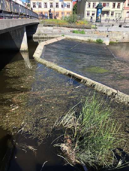
Modelling the risk of rainfall events
 leading to momentary pollution
         levels exceeding
 maximum allowed concentrations
  A Swedish case study of urban runoff in the Fyris river

                  Tove Gannholm Johansson

                  Supervisor: Hannes Öckerman

                  Subject reader: Thomas Grabs

                           2021-05-26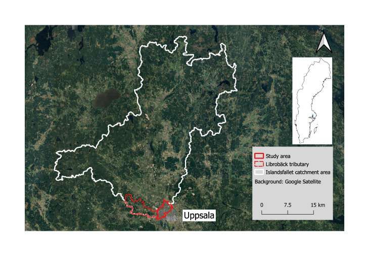
Abstract
Modelling the risk of rainfall events leading to momentary pollution levels
exceeding maximum allowed concentrations
- A Swedish case study of urban runoff in the Fyris river
Tove Gannholm Johansson

The purpose of this study was (1) to study the proportion (X) of the flow in a wa-
tercourse that consists of urban runoff during a rain event and (2) to evaluate the
risk that a few chosen pollutants, transported by urban runoff, exceed the maximum
allowed concentration in the watercourse according to the environmental quality stan-
dards (MAC-EQS). The Fyris river in Uppsala, Sweden, was selected as a case study.

Urban runoff quickflow was estimated with a water balance model using precipitation
data and flow data from three stations. Precipitation data was used to identify 31 rain
events with a minimum rain volume of 10 mm and at least a maximum rain intensity
of three mm/h during the study period 2017-2020. Pollutants in urban runoff were
sampled during the winter of 2020-2021. The highest concentrations obtained during
sampling were used to estimate momentary pollution concentration and to evaluate
the risk of exceeding MAC-EQS.

The highest X found during a rain event was 71%. Low flow conditions in the river
prior to a rain event in summertime are circumstances when X can be expected to
be high. It is therefore advised to include rain events under such circumstances when
monitoring MAC-EQS or sampling momentary pollution concentrations in the Fyris
river.

The pollutant category polycyclic aromatic hydrocarbons (PAH), and especially the
pollutant fluoranthene, showed risk of momentary pollution concentration exceeding
MAC-EQS. The highest risk was observed in the Luthagen catchment area. Therefore,
the author recommends that mitigation measures for urban runoff should be consid-
ered and include PAHs.

Keywords: urban runoff, flow, rain event, pollution concentration, EQS, MAC-EQS
Department of Earth Sciences, Program for Air, Water and Landscape Science,
Uppsala University, Villavägen 16, SE-752 36, Uppsala, ISSN 1401-5765
Referat
Modellering av risken att regntillfällen leder till tillfälliga förorenings-
koncentrationer som överskriver maximala tillåtna koncentrationer
- En svensk fallstudie av dagvatten i Fyrisån
Tove Gannholm Johansson

Syftet med denna studie var (1) att studera hur stor andel (X) av flödet i ett vat-
tendrag som utgörs av dagvatten vid ett regntillfälle, och (2) att utvärdera risken att
ett utvalt antal föroreningar som transporteras med dagvattnet överskrider maximal
tillåten koncentration enligt miljökvalitetsnormerna för vatten (MAC-MKN). Fyrisån
i Uppsala, Sverige, valdes som fallstudie.

Snabbt dagvattenflöde (quickflow) uppskattades med en vattenbalansmodell som an-
vände nederbördsdata samt vattenföring från tre stationer. Nederbördsdata användes
för att identifiera 31 regntillfällen med en minsta regnvolym på 10 mm och minst en
maximal regnintensitet på tre mm/h under perioden 2017-2020. Föroreningar i dagvat-
ten provtogs under vintern 2020-2021. De högsta koncentrationerna som påträffades
vid provtagningen användes för att uppskatta momentan föroreningskoncentration och
för att utvärdera risken att MAC-MKN överskrids.

Det högsta X som beräknades under ett regntillfälle var 71%. Lågt flöde i Fyrisån in-
nan ett regntillfälle under sommartid är omständigheter när X kan förväntas vara högt.
Det rekommenderas därför att inkludera regntillfällen under sådana omständigheter
när MAC-MKN övervakas eller när momentana föroreningskoncentrationer i Fyrisån
provtas.

Föroreningskategorin polycykliska aromatiska kolväten (PAH), och särskilt förorenin-
gen fluoranten, uppvisade risker för att MAC-MKN skulle överskridas. Den högsta
risken identifierades för avrinningsområdet Luthagen. Därför rekommenderas att ren-
ingsåtgärder för dagvatten bör övervägas och inkludera avskiljning av PAH:er.

Nyckelord: dagvatten, flöde, regntillfälle, föroreningskoncentration, MKN,
MAC-MKN
Institutionen för geovetenskaper, Luft-, vatten- och landskapslära, Uppsala Universitet
Geocentrum, Villavägen 16, SE-752 36, Uppsala, ISSN 1401-5765

Populärvetenskaplig sammanfattning

Våra vattendrag är viktiga eftersom de bidrar med betydelsefulla ekosystemtjänster
såsom dricksvatten, biologisk mångfald, livsmiljöer för många vatten- och landlevande
organismer samt rekreation. Tyvärr är många vattendrag känsliga för föroreningar
som bland annat transporteras från städer och försämrar vattenkvaliteten. För att
skydda våra vatten mot dålig vattenkvalitet finns lagstiftning som bland annat in-
nehåller gränsvärden för vilka föroreningskoncentrationer som får finnas i ett vatten-
drag (miljökvalitetsnormer). Dessa gränsvärden finns både som årsmedelvärden och
som maximal tillåten koncentration.

När det regnar i en stadsmiljö rinner vatten av från ytor och tar med sig smuts och
föroreningar ner i vattendrag. Denna avrinning kallas dagvatten. Idag används of-
tast årsmedelvärden av föroreningars koncentrationer för att utvärdera dagvattnets
påverkan på vattendrag, till exempel vid exploatering av ett nytt bostadsområde.
Dagvatten tillkommer dock inte jämnt fördelat över året utan i tillfälliga pulser när
det regnar eller när snö smälter. Därför kan det skapas kortvariga, höga föroren-
ingskoncentrationer i ett vattendrag. Det finns idag förhållandevis lite kunskap om
sådana föroreningstoppar i vattendrag eftersom det är kostsamt och tidskrävande att
provta och analysera många vattenprover.

För att försöka uppskatta dessa tillfälliga toppar av föroreningskoncentration i ett
vattendrag, undersöker denna studie om det finns ett användbart samband mellan
regntillfälle och andelen dagvatten i ett vattendrag. En vattenbalansmodell användes
tillsammans med nederbörds- och flödesdata från Fyrisån i Uppsala 2017-2020. Den
största andelen dagvatten som hittades i studien var 71%. Andelen dagvatten kan
antas vara hög när det är lågt flöde inför ett regn i Fyrisån under sommartid. Därför
rekommenderas att övervakning av gränsvärden och provtagning sker just under som-
martid när det är lågt flöde i Fyrisån.

Studien undersökte också risken för att miljökvalitetsnormer skulle överskridas av
tillfälliga föroreningstoppar under regntillfällen. Provtagning av dagvatten genom-
fördes under vintern 2020-2021. Studien visade på att det fanns en risk att de organiska
föroreningarna polycykliska aromatiska kolväten, PAH:er, och särskilt föroreningen flu-
oranten, kan överskrida miljökvalitetsnormerna. Störst risk identifierades i avrinning-
sområdet för Luthagen. Därför rekommenderas att dagvattenåtgärder bör övervägas
och inkludera avskiljning av PAH:er.

Det kvarstår emellertid många frågor kring föroreningskoncentrationen i ett vattendrag
vid ett regntillfälle och mer forskning behövs för att hitta ett användbart samband som
kan förutsäga tillfälliga föroreningskoncentrationer i vattendrag.
Preface
This work was written as a 30 credit master thesis, concluding the Master of Sci-
ence program in Water and Environmental Engineering at Uppsala University and the
Swedish University of Agricultural Sciences. The project was initiated by WRS and
supervised by Hannes Öckerman from WRS. The subject reader was Thomas Grabs,
Senior lecturer/Associate Professor at the Department of Earth Sciences, Program for
Air, Water and Landscape Sciences; Hydrology at Uppsala University.

I would like to thank the team at WRS for always being a source of inspiration and
for providing equipment and data. A special thank you to my supervisor Hannes Öck-
erman and subject reader Thomas Grabs for interesting and helpful discussions.

A big thank you to Jenny Näslund at WRS for organising the sampling and to my
master thesis colleague Matilda Ahlström, who’s cheerfulness got us through those
rainy days of sampling.

I would lastly like to express my gratitude to friends and family who have encouraged
me and believed in my capabilities to undertake this project.

Tove Gannholm Johansson
Uppsala, June 2021

Copyright © Tove Gannholm, WRS and Department of Earth Sciences, Air, Water
and Landscape Science, Uppsala University. UPTEC W 21019 ISSN 1401-5765. Dig-
itally published in DiVA, 2021, through the Department of Earth Sciences, Uppsala
University. (http://www.diva-portal.org/)
Definitions
’young’ water Water from a recent rain event
ADWP Antecedant dry weather period. The period before a rain event with no
   precipitation
baseflow Flow caused by processes which mobilize deliver water slowly to a water-
     course
duration The time duration of a rain event
EQS Environmental Quality Standard
first flush effect The initial runoff during a rain event which has the potential to
      transport a large part of the total pollution load
fraction In what form the substance can be found. For example particulate
HaV The Swedish Agency for Marine and Water Management
hydrograph Graph of flow over time
hydrograph separation Method for separating the hydrograph into quickflow and
    baseflow. Can be graphical or tracer-based
landuse The main characteristics of an area. For example forest or residential area
MAC-EQS Maximum Allowed Concentration Environmental Quality Standard
PAH Polycyclic Aromatic Hydrocarbon. A group of pollutants
precipitation Rain and snow
Q Water flow
quickflow Flow caused by processes which mobilize water quickly to a watercourse
rain depth The rain volume referred to as a depth [mm]
rain event An occasion when it rains. A definition used in this project for analysing
     purposes with certain conditions
rain intensity The rain depth during one hour [mm/h]
residence time How long a substance spends in a lake or reservoir
runoff coefficient Used to predict how much runoff is created from precipitation
SMHI The Swedish Meteorological and Hydrological Institute
urban runoff Runoff from rain or snowmelt in an urban area
water balance Mass balance for water
WFD Water Framework Directive
X The maximum proportion of urban runoff during a rain event
Contents
1 Introduction                                                                                             1
  1.1 Aim and Research Questions . . . . . . . . . . . . . . . . . . . . . . . .                           1

2 Background                                                                                               2
  2.1 Urban hydrology and urban runoff . . . . . . . . . . . . .              .   .   .   .   .   .   .    2
  2.2 Rain event . . . . . . . . . . . . . . . . . . . . . . . . . . .        .   .   .   .   .   .   .    3
  2.3 Hydrograph . . . . . . . . . . . . . . . . . . . . . . . . . .          .   .   .   .   .   .   .    4
  2.4 Hydrograph separation . . . . . . . . . . . . . . . . . . . .           .   .   .   .   .   .   .    5
  2.5 Runoff coefficients . . . . . . . . . . . . . . . . . . . . . . .       .   .   .   .   .   .   .    6
  2.6 Urban runoff water quality . . . . . . . . . . . . . . . . . .          .   .   .   .   .   .   .    6
  2.7 First flush effect . . . . . . . . . . . . . . . . . . . . . . . .      .   .   .   .   .   .   .    8
  2.8 Effects on biota . . . . . . . . . . . . . . . . . . . . . . . .        .   .   .   .   .   .   .    8
  2.9 Environmental quality standards for water . . . . . . . . .             .   .   .   .   .   .   .    9
       2.9.1 Swedish pollution concentration modelling practices              .   .   .   .   .   .   .    9
  2.10 Hydrological modelling tools . . . . . . . . . . . . . . . . .         .   .   .   .   .   .   .   10
       2.10.1 Water balance . . . . . . . . . . . . . . . . . . . . .         .   .   .   .   .   .   .   10
       2.10.2 Concentration and mixing . . . . . . . . . . . . . .            .   .   .   .   .   .   .   11
       2.10.3 Residence time . . . . . . . . . . . . . . . . . . . .          .   .   .   .   .   .   .   12

3 Material and Methods                                                                                    12
  3.1 Description of Study Area . . . . . . . . . . . . . . . . .         .   .   .   .   .   .   .   .   12
  3.2 Data . . . . . . . . . . . . . . . . . . . . . . . . . . . . .      .   .   .   .   .   .   .   .   16
  3.3 Methods . . . . . . . . . . . . . . . . . . . . . . . . . . .       .   .   .   .   .   .   .   .   18
      3.3.1 Modelling the proportion of urban runoff . . . . .            .   .   .   .   .   .   .   .   18
      3.3.2 Estimation of momentary pollution concentration               .   .   .   .   .   .   .   .   24

4 Results                                                                          25
  4.1 Proportion of urban runoff . . . . . . . . . . . . . . . . . . . . . . . . . 25
  4.2 Momentary pollution concentrations . . . . . . . . . . . . . . . . . . . 33

5 Discussion                                                                                              36
  5.1 Proportion of urban runoff . . . . . . .      . . . . . . . . . .   .   .   .   .   .   .   .   .   36
      5.1.1 Methodology discussion . . . .          . . . . . . . . . .   .   .   .   .   .   .   .   .   36
      5.1.2 Results, future perspectives and       recommendations        .   .   .   .   .   .   .   .   38
  5.2 Momentary pollution concentrations .          . . . . . . . . . .   .   .   .   .   .   .   .   .   39
      5.2.1 Methodology discussion . . . .          . . . . . . . . . .   .   .   .   .   .   .   .   .   39
      5.2.2 Results, future perspectives and       recommendations        .   .   .   .   .   .   .   .   41

6 Conclusion and future perspectives                                                                      43

References                                                                            44
  Published . . . . . . . . . . . . . . . . . . . . . . . . . . . . . . . . . . . . . 44
  Unpublished . . . . . . . . . . . . . . . . . . . . . . . . . . . . . . . . . . . . 46

Appendices                                                                                                 i

A Study area                                                                                               i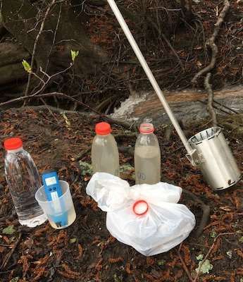
B Sampling procedure                               v

C Estimation of flow from Librobäck tributary     xi

D Parameters                                     xiv

E Rain events                                   xviii
1     Introduction
Watercourses are a valuable asset in today’s society, providing us with essential ecosys-
tem services such as drinking water, biodiversity, habitat for flora and fauna, as well as
human recreation (HaV 2017). For all of these ecosystem services, a good water qual-
ity is vital. To ensure a good water quality, the Water Framework Directive (WFD)
was adopted by EU in 2000 (2000/60/EC). In Sweden, the Swedish Agency for Ma-
rine and Water Management (HaV) is responsible for the Swedish implementation of
the WFD and it has issued limits for pollution concentrations called Environmental
Quality Standards (EQS). There are both limits for yearly average concentrations and
maximum allowed concentrations (MAC-EQS) (HaV 2019).

Today, pollution of watercourses from urban runoff is often modelled as yearly average
concentration. However, urban runoff primarily reaches watercourses during individ-
ual rain events. As the urban runoff arrives in pulses, the consequence is that the
momentary effect on the watercourse might be considerably larger than the yearly
average. Since random sampling of urban runoff does not give representative values
and analysing many samples is expensive (Fölster et al. 2019) there is little knowledge
on momentary pollutant concentrations in watercourses due to urban runoff. It is
therefore valuable to examine whether momentary pollutant concentrations could be
toxic to the aquatic environment and/or exceed the environmental quality standards
for waters.

To increase knowledge of when high momentary pollutant concentrations occur, there
is a need to study the impact of different rain events and flow situations in water-
courses. Finding a way to estimate the momentary pollution in a watercourse can
bring knowledge and possibly save money. Ideally, one way could be to reliably de-
termine the proportion of urban runoff in the watercourse. Known urban runoff con-
centrations during rain events could then be used to estimate momentary pollution
concentrations. The combined information of momentary proportions of urban runoff
and momentary pollution concentrations in the watercourse, would allow to prioritise
which future urban runoff mitigation measurements are needed.

1.1     Aim and Research Questions
The main aim of this report is to estimate momentary concentration of pollutants
in the watercourse and evaluate if these risk exceeding MAC-EQS. To estimate the
momentary pollutant concentration, a model is needed. Therefore, the second aim
of this report is to create a model from flow and rain data, which can predict the
proportion of flow in a watercourse originating from urban runoff, during different rain
events. This model will then be combined with urban runoff concentrations sampled
in this study. For this project, the river Fyris in Uppsala is used as a pilot study. To
achieve the aim, the following questions were developed.

    1. What proportion of the flow in the Fyris river is made up of urban runoff at a
       rain event?

    2. Do momentary pollutant concentrations in the river risk exceeding MAC-EQS?

                                            1
2 Background
In this section, background knowledge and the current research situation is presented.
First, following the path of a raindrop from rain to flow, then water quality and the
EQS for water, and last some hydrological modelling tools.
2.1 Urban hydrology and urban runoff
Runoff from rain or snowmelt in an urban area is called urban runoff. As an urban
area develops, previously permeable natural surfaces are built on and made impervi-
ous, which changes the natural hydrology to urban hydrology (Swedish Water 2011).
Urban hydrology is characterised by decreased infiltration and an increase in surface
runoff, both in intensity and volume (ibid.), see Figure 1 for a simplified illustration.
This can affect both the magnitude of water flow and pollution concentrations in re-
ceiving waters (ibid.). Pollutants can originate from for example roads, roofs or other
urban surfaces.
The focus in urban runoff management and design in Sweden has historically been to
avoiding floodrisks. However, designing systems for both flood and pollution mitiga-
tion has developed in the last few decades (Swedish Water 2004, 2011, 2016). There-
fore, many urban areas lack the infrastructure needed to mitigate the environmental
effects of urban hydrology, such as polluted runoff.
This study focuses on urban catchments in Uppsala in which few urban runoff mitiga-
tion measures, such as stormwater ponds, exist and the effects on the receiving water
body could possibly be large. For more information on urban runoff management
in Uppsala and good examples of urban runoff infrastructure, see Uppsala Vatten’s
reference manual (2014) and example collection (2014).
Figure 1: Simplified illustration of urban hydrology compared to natural hydrology.
22.2 Rain event
What is a rain event? The simple answer is when it is raining. However, rain events
can vary both spatially and temporally, and in intensity and duration (Swedish Water
2011). Therefore, rain event as a term needs to be specified.
Rain or precipitation can be measured at stations using weighing buckets or tipping
buckets (SMHI 2021a; Swedish Water 2011). They can be heated (Jansson 2021;
SMHI 2021a) or contain defrosting chemicals (SMHI 2021a) to account for snowfall.
The Swedish Meteorological and Hydrological Institute (SMHI) mostly uses weighing
buckets while some municipalities use tipping buckets. The latter option is cheaper
but can have uncertainties due to evaporation or loss of rain volume when the tipping
buckets overflow during intense rains (ibid.).
There are other uncertainties associated with precipitation measurements (SMHI 2021a;
Swedish Water 2011). Wind turbulence at the measuring station can affect the mea-
surement and therefore a good placement of the station in a big open area is critical
(SMHI 2021a). This is sometimes difficult in an urban setting with dense housing.
Snow is problematic as it can clog the inlet to the measuring instrument if it is un-
heated (ibid.).
In water balance studies, the actual measured precipitation is often corrected using air
temperature, wind speed, type of precipitation and type of measuring instrument but
SMHI publishes uncorrected data (ibid.). A difference in volume is often found when
comparing municipal tipping bucket data with SMHI station data but correcting data
straight off with a statistical correction term is not recommended for high-resolution
data (Swedish Water 2011). When analysing rain events for urban runoff purposes,
high-resolution data is recommended as important information like rain intensity might
otherwise be lost (ibid.). Rain is spatially unevenly distributed and there can be great
variations even on a local scale (ibid.). Therefore, having a local network of measuring
stations can be beneficial (ibid.). Measurements from several rain gauges can be dis-
tributed spatially over the study area in order to obtain representative data. If using an
arithmetic mean, spatial information is lost in the process. Thiessen polygons on the
other hand, also know as voronoi polygons, is a method which takes spatial information
into account and which can be suitable for a relatively flat study area (Hendriks 2010).
Furthermore, data might need to be paired with temperature data and some knowledge
of snow to distinguish rain events from snowfall and snowmelt in the measuring equip-
ment. In contrast to rain, snow remains stored for extended periods, and accumulates
pollutants over a longer time (Vijayan 2020). This indicates that urban runoff from
snowmelt should be studied separately from rain events, to reliably estimate pollutant
transport processes.
Moreover, rain event duration need to be established. To distinguish two separate
rain events for analysis purpose, certain time must pass since the end of the last rain
event. Previously used break durations have been between 2 and 36 hours, where 2 - 6
hours are normally used in rain data analyses in Sweden (Swedish Water 2011). Other
3studies or projects have used 6 h (Larm & Blecken 2019) and 12 h (Öckerman 2021).
Rain events can also be classified according to total volume, intensity and duration
(Swedish Water 2011). When the first raindrops fall on a dry surface, the rain wets
the surface and fills up small pores and an initial rain volume does not create runoff
(ibid.). Therefore, rain events with very low intensity or total rain volume might not
produce much urban runoff, especially if there has been a longer time since the last
wetting, the antecedent dry weather period (ADWP). So for urban runoff purposes,
there is reason to set a minimum intensity or volume level for rain events being studied.
Previously used limits are > 0.2 - 2 mm (Larm & Blecken 2019; Scherling, Svensson,
& Sörelius 2020; Swedish Water 2011; Zgheib et al. 2011).
2.3 Hydrograph
A graph of flow (Q) over time is called a hydrograph (Hendriks 2010), see Figure 2.
A hydrograph is often shown together with a hyetograph, precipitation over time, to
visually illustrate the link between precipitation and flow. The flow can be divided
into two different categories depending on the flow behaviour. Quickflow is caused
by processes which mobilize water quickly to the watercourse, such as rapid soilwater
throughflow, pipeflow or channel precipitation. While the afformentioned processes
mobilize relatively ’young’ water to the streams, quickflow can also be caused by pro-
cesses such as the transmissitivity feedback that mobilize ’old’ water. Such processes
can be important for the runoff chemistry (Bishop et al. 2004). The other flow category
is called baseflow. Baseflow is caused by processes which deliver water more slowly to
the watercourse, continuously delivering water also during dry periods. Examples of
such slow processes are slow soilwater throughflow and groundwater flow during dry
periods (Hendriks 2010). In this study it is assumed that quickflow from urban areas
is mostly associated with processes such as overland flow or pipeflow which deliver
mostly ’young’ water to the recipients.
A common hydrograph has some key characteristics. Before a rain event, there is base-
flow recession (there is only baseflow and it is declining). When a rain event occurs,
the flow increases until a peak flow (maximum quickflow) is reached. The flow then de-
creases until a separation point is reached, when there is again only baseflow recession.
4Figure 2: Hydrograph.
A study used a hydrograph to predict event based pollutants coming from urban catch-
ments (Tao et al. 2019). They found it feasible that a hydrograph can predict event
based pollutant loads to receiving waters (ibid.). The study suggests that once a yield
function has been established for the catchment, rain data can be used to estimate
pollutant load to receiving waters and therefore reducing the need to monitoring the
pollutant load by sampling at each rain event (ibid.).
Both the hydrograph and the pollutograph, depicting pollutant concentration over
time, depend on parameters such as rainfall intensity, ADWP, antecedent rainfall and
the characteristics of the catchment (Bertrand-Krajewski, Chebbo, & Saget 1998).
2.4 Hydrograph separation
A hydrograph separation aims at separating the hydrograph into baseflow and quick-
flow. There are two types of hydrograph separation, graphical and tracer-based. A
tracer-based method entails measuring some water quality parameter, for example
conductivity (Hendriks 2010) or isotope composition (Grip & Rodhe 2016), in the wa-
tercourse and in sources and pairing this with a hydrograph, while a graphical method
separates the hydrograph graphically, based only on the hydrograph. A tracer-based
method would have been preferable for this study because it is process-based and it is
used to trace the age and sources of the water. However, in the absence of tracer data,
the choice fell on a graphical method, under the previously mentioned assumption, see
previous section, that quickflow is assumed to be ’young’ water delivered by pipeflow
and overland flow.
There are several methods for graphical hydrograph separation and most are arbitrary
(Hendriks 2010). The most important aspect when doing a graphical hydrograph sep-
aration is to use the same method consistently to make comparison possible (ibid.).
Examples of graphical methods are the constant discharge method, the constant-slope
separation point method and the concave curve separation point method (ibid.).
5Lyne and Hollick (Lyne & Hollick) suggested using a digital filter for hydrograph
separation. The Lyne and Hollick filter has later been standardised (Ladson et al.
2013). Advantages of using a standardised filter is that the result of the hydrograph
separation is reproducible and comparable, and that suitable parameter values are
suggested (ibid.). An example using the standardised Lyne and Hollick filter can be
found on the author’s website 1 . The parameters used in the standard filter are α, the
number of values reflected at the start and end of the time series, and the number of
passes back and forth (ibid.). The recommended α is 0.98 but 0.925 has been used
historically (ibid.). α should be calibrated with tracers if possible (ibid.). The number
of reflected days recommended is 30 (ibid.). The number of passes has to be uneven,
with 3 passes being recommended for daily data resolution and 9 passes for hourly
data resolution (ibid.).
2.5 Runoff coefficients
Runoff coefficients are used to predict how much runoff is created from precipitation.
The higher the runoff coefficient, the more runoff is created. They can be site specific
or based on landuse. Runoff coefficients are often higher for hardened surfaces than for
natural landuse and there, agricultural land have higher runoff coefficients than forest
(Swedish Water 2016). However, natural landuse can also have high runoff coefficients
on occasion. At high rain intensities or big rain volumes, the ground can become
saturated which means more runoff is created (ibid.).
The landuse based runoff coefficients provided by Swedish Water account for the de-
gree of exploitation, impervious surfaces and the slope of the landscape (Swedish Water
2004, 2016). The stormwater model StormTac also provides data on runoff coefficients
based on data from long time flow proportional sampling and urban runoff analysis
(StormTac 2021).
A recent study in Stockholm found that standard runoff coefficients were larger than
the runoff coefficients calculated in the study (Rennerfelt et al. 2020).
2.6 Urban runoff water quality
Summarising urban runoff water quality is difficult since the pollutant types are abun-
dant, and there are numerous factors which can affect the presence of pollutants.
The most important pollutants in urban runoff are those which are usually found in
an urban setting. They are common and/or persistent heavy metals or organic sub-
stances, often harmful to the environment. E. Eriksson et al. suggested 25 prioritised
urban runoff pollutants to be included when evaluating risks from urban runoff (2007).
Among the 25 pollutants were metals (Cd, Cr, Cu, Ni, Pb, Pt and Zn) and PAHs.
This list of pollutants might have to be complemented with locally present pollutants.
To study the presence of pollutants, a study of a Parisian suburb examined 88 pollu-
tants(Zgheib et al. 2011). Of these, 45 were found in urban runoff (ibid.). A majority
1
(https://tonyladson.wordpress.com/2013/10/01/a-standard-approach-to-baseflow-separation-
using-the-lyne-and-hollick-filter/)
6of the pollutants found are monitored by the WFD but some are not included (Zgheib
et al. 2011), for example PBCs, historically used in electrical applications.
Common urban runoff pollutants come in different fractions, where a standardised
separation is made between the dissolved and the particulate fraction. The dissolved
fraction consists of pollutants that remain when the analysed water is filtered through
a 0.45 µm filter, and the particulate fraction cannot pass through the filter. Total
concentrations refer to both fractions. The occurrence of pollutants in urban runoff
can depend on which fraction is analysed (ibid.).
In a study from southeastern France, rain events were found to contribute with 90%
of the annual output of particulate Cu, Zn, Cd and Pb and more than 60 % of the
dissolved fraction (Nicolau, Lucas, et al. 2012). The study was carried out for rain
events with a minimum total volume of 11 mm but with no clear definition of ADWP
(ibid.). The correlation of parameters varied greatly between different rain events
(ibid.). However, rainfall intensity, antecedent rainfall history and season were able to
explain observed variations sufficiently (ibid.). Metals were mostly transported in the
particulate fraction (ibid.).
The concentration in watercourses can vary greatly due to urban runoff pulses and
therefore it is not possible to take representative random samples for urban runoff
(Fölster et al. 2019). In other words, the pollution concentrations in watercourses can
be different before and during a rain event. Additionally, a study from China found
significant temporal and spatial variations in the pollutant wash-off process during the
rain events (D. Li et al. 2015), i.e. two rain events can give different urban runoff
concentrations and the concentration can differ for two catchment areas during the
same rain event.
In the watercourse, point sources can contribute to an uneven pollutant distribution,
in the water column depth and across the watercourse. This was for example seen in
a study of micro plastics (Bondelind et al. 2020). The contribution of point sources
at rain events can be visually seen in the change in water colour upstream and down-
stream of major urban runoff outlets in the Fyris river (Andersson 2021).
A study of an urban area river in France found alarming momentary metal concentra-
tions (Nicolau, Galera-Cunha, & Lucas 2006). The study showed that low flow (base-
flow) during non-rainy periods had low pollutant concentrations while heavy rains after
dry periods, with high flow had higher pollutant concentrations (ibid.). Some metals
were found in concentrations which can affect biota (ibid.). A seasonal dilution effect
was seen for metals, where concentrations were lower during high flow periods (ibid.).
A case study in Uppsala found heavy metal concentrations in urban runoff decreased
with a higher proportion of urban runoff baseflow (Karlsson & Öckerman 2016). The
study found that concentrations of Pb, Cu and Zn greatly exceeded values in the Fyris
river (ibid.). The study suggests the accumulation of heavy metals in the catchment
area is important for the pollutant concentration at a certain rain event (ibid.), i.e.
ADWP.
7In brief, there are at least 25 pollutants which are highly relevant when studying urban
runoff. The factors which affect their presence can be time related, location related,
fraction related, and all of these relations can vary with pollutant.
2.7 First flush effect
Many studies refer to the so-called first flush effect. It is the initial runoff during a
rain event which has the potential to transport a large part of the total pollution load.
Both urban runoff event mean-concentrations and first-flush-40 (the first 40% of total
runoff volume) have been found to correlate with maximum rain intensity, mean rain
intensity, total rain volume and ADWP (D. Li et al. 2015). Another study uses the
term first-flush-30, where it is said to be significant if 80% of the total pollutant mass
is transported in this first flush (Bertrand-Krajewski, Chebbo, & Saget 1998). A study
from France suggests this first flush is rare, however (ibid.).
Nevertheless, the same study found some first flush effects. In separate sewer systems
(where stormwater is transported separately from the wastewater) 50% of the pollu-
tant mass was transported in the first 38% of the total volume for 50% for the rain
events, and 80% was transported in the first 74% (ibid.). The first flush depends on
the site, pollutant, rain event and the sewer system (ibid.).
A study in Los Angeles found that particles showed a strong first flush effect where
40% of the particles were transported in the first 20% of the runoff volume (Y. Li et al.
2005).
2.8 Effects on biota
Several pollutants are potentially toxic to biota. In this context, the most common
metals are Pb, Cd, Co, Cu, Cr, Hg, Ni, Ag, Sn, V and Zn (Naturvårdsverket 2008).
They can for example damage the nerves, vital organs or cause reproductive issues
ibid. Another pollutant type is PAH, which are carcinogenic organic substances ibid.
Because pollutants are often persistent, many can bioaccumulate, which means the
pollutant can be found in greater concentrations in organisms compared to in the wa-
ter. They can also biomagnify, meaning the concentration is higher in top-organisms
such as predators. As a consequence, concentrations in the water which are not con-
sidered toxic can lead to toxic concentrations in biota over time.
Previously, the fraction of the total pollution concentration which could affect the
biota was considered to be the dissolved fraction. However, today only a part of the
dissolved fraction is considered potentially toxic to aquatic organisms and this fraction
is referred to as the bioavailable fraction (HaV 2019).
Bioavailable concentrations should be calculated with an appropriate methods or mod-
els (HaV 2013). For Cu, Zn and Ni, the bioavailable concentration can be calculated
8using the biomet bioavailability tool which is a biotic ligand model (BLM) (Bio-met
2019). It uses total concentrations, DOC, pH and Ca as parameters (ibid.).
2.9 Environmental quality standards for water
The Water Framework Directive (WFD) 2000/60/EC exists to protect European wa-
ters (The European parliament and the Council of the European Union 2000). A goal
of the WFD is that all surface waters should achieve at least good ecological status
(GES), or good ecological potential, and good chemical status (GCS) (ibid.). The en-
vironmental quality standards (EQS) are a measurement tool to fulfil the goal of the
WFD. An EQS is "the concentration of a particular pollutant or group of pollutants
in water, sediment or biota which should not be exceeded in order to protect human
health and the environment" (ibid.). The EQS for individual surface waters are de-
fined based on how impacted the surface waters are by human activity, their ecological
status, ecological potential, chemical status and a risk evaluation (HaV 2019).
The EQS for some common urban runoff pollutants for the Fyris river to achieve
GES and GCS are presented in Table 1. Pollutants include some metals as well as
two polycyclic aromatic hydrocarbons (PAH) for which the Fyris river do not achieve
GCS; anthracene and fluoranthene (VISS n.d.). The EQS are given as annual average
(AA) concentration and for some pollutants maximum allowed concentration (MAC)
(HaV 2019). The EQS for the metals refer to the dissolved concentration and for Pb,
Cu, Zn and Ni they refer to the bioavailable dissolved concentrations for the annual
average concentration (ibid.). The EQS for Cd depends on the hardness of the water
and is divided into 5 classes where the Fyris river falls into class 4 (VISS n.d.).
Table 1: Common urban runoff pollutants and their respective EQS, annual average AA-EQS and
maximum allowed concentration MAC-EQS (HaV 2019).
AA-EQS MAC-EQS
Pollutant
[µg/L] [µg/L]
TotP
Pb 1.2 bioavailable 14
Cu 0.5 bioavailable
Zn 5.5 bioavailable
Cd 0.15 (class 4) 0.9 (class 4)
Cr 3.4
Ni 4 bioavailable 34
Anthracene 0.1 0.1
Fluoranthene 0.0063 0.12
BaP 0.00017 0.27
2.9.1 Swedish pollution concentration modelling practices
The informal Swedish practice for calculating and evaluating pollution concentrations
from urban runoff generally does not take into consideration the risk of momentary pol-
lution from rain events. Usually, the annual average pollutant concentrations and/or
9annual pollutant loads are calculated when evaluating the environmental impact of
urban runoff. When modelling pollution concentrations, Swedish Water suggests look-
ing at StormTac values for pollution concentrations (Swedish Water 2016) and the
Stormtac database contain yearly average pollution concentrations, based on landuse
type (StormTac 2021).
2.10 Hydrological modelling tools
Models can be more or less complicated, demanding and useful in terms of uncertain-
ties and output. When choosing a model, pros and cons of models should be weighed
against the purpose of the model and what is required to achieve this purpose. Model
categories that were considered for this project include distributed models and lumped
models.
Distributed models take spatial variation into account (Hendriks 2010). Examples of
distributed models are MIKE and SWMM which have integrated powerful calculation
tools and give spatial resolution. However, they require more input data and are hard
to calibrate and validate. Consequently, the output from a distributed model might
be uncertain if data is not sufficient.
Lumped models are spatially averaged (ibid.). For water flow, lumped models can
be visualised as a bucket with inflow and outflow where the processes in the bucket
cannot be distinguished. Lumped models usually require less data input and are there-
fore more manageable and often easier to calibrate and/or validate than distributed
models. Therefore, the output of a lumped model can have less uncertainties than for
a distributed model. On the other hand, lumped models do not provide any spatial
resolution. Nonetheless, the spatially averaged output from a lumped model can still
be satisfactory for the purpose of the project.
2.10.1 Water balance
A mass balance model is based on the law of conservation of mass and can be applied to
water or pollution concentrations. The water balance entails all that inflows of water
Qin must equal all outflows Qout plus the difference in storage ∆S/∆t, see Equation
1 (Hendriks 2010). Put in a model frame, data on available inflows and outflows are
input parameters and the output is the flow, in this case urban runoff contribution
from a rain event.
X X ∆S
Qin = Qout + (1)
∆t
When setting up a water balance, it is important to consider all possible flows and
the storage difference (ibid.). The flows taken into consideration for a surface water in
Hendriks’s drainage basin hydrological system (2010) are discharge, channel precipi-
tation, overland flow, flooding, evaporation, soil water throughflow and ground water
flow and recharge, see Figure 3.
10Figure 3: The hydrological system of surface water, based on Hendriks (2010), as a water balance
in a lumped model. The blue surface water can be visually represented as a bucket with inflows and
outflows. Arrows pointing to the surface water are inflows and arrows pointing from the surface water
are outflows.
2.10.2 Concentration and mixing
A pollutant concentration can be calculated by the conservation of mass, see Equa-
tion 2. The mixing model used in this study assumes that the water body is mixed
completely, and that mass is constant, i.e. no mass is added or removed by reactions
or changes to particulate or dissolved fraction. This mixing model will be referred to
as a conservative mixing model.
V1 · c1 + V2 · c2 = V3 · c3 (2)
However, the pollutant concentration in a river can vary between different parts of the
water volume due to mixing. If water volumes do not mix, streaking can occur with
big concentration gradients, see Figure 4. Downstream of waterfalls or weirs, there
is often turbulent water. Turbulence increase mixing in the water column and it is
common practice to assume complete mixing has occurred downstream of a fall or weir.
Stratification is likely to appear in slow moving water in deep lakes or reservoirs. Tem-
perature differences between top layers of the water column in contact with the atmo-
sphere, and deeper layers can cause stratification. Sweden has a dimictic stratification
pattern were the entire water column mix in spring and in autumn and stratification
is common in winter and in summer.
Figure 4: Illustration of how complete mixing, streaking or stratification affect the concentration in
a river.
In a river, reactions or fraction changes might occur. Changes in water velocity and
turbulence can cause particles to sediment or resuspend and water quality parameters
11such as pH or the chemical composition can affect solubility. If these processes are not
in equilibrium, conservative mixing cannot be assumed.
2.10.3 Residence time
The residence time of a lake or reservoir describes how long time a substance or a
water molecule on average spend in the lake or reservoir. The residence time (τ ) can
be calculated as the reservoir volume (Vreservoir ) divided by the outflow (Qout ) (NE
n.d.), see Equation 3. If τ is small, then the water in the reservoir is quickly replaced
with new water.
Vreservoir
τ= (3)
Qout
3 Material and Methods
In this section, the study area, the data material and the methods used in this project
are presented.
3.1 Description of Study Area
The Fyris river is located in Uppland in Sweden passes through the city of Uppsala,
almost at the end of its course. The Fyris river has moderate ecological status ac-
cording to the WFD (VISS n.d.) and is therefore sensitive to pollutants from urban
runoff. The Fyris river drains a total catchment area of 2002 km2 into lake Ekoln
(Uppsala University 2021) which is part of lake Mälaren, a drinking water source for
the city of Stockholm. Uppsala is the biggest city in the Fyris river catchment area
with a population of 240 000 inhabitants. Uppsala has an annual total precipitation
of 623 mm which is predicted to increase with 20 - 30% (SMHI 2015) to 2100. More
extreme weather events due to climate change are also predicted (ibid.). The elevation
ranges from 7 to 107 m.a.s.l. Forest and agriculture are the dominating land covers
in the catchment. There is an esker that runs along the river Fyris and through the
city. The Fyris river catchment area upstream of the study area can be seen in Figure 5
12Figure 5: The study area in red, and the Librobäck catchment area in dotted red line. The entire
catchment area upstream of Islandsfallet in white. Small map of Sweden: Uppsala is located in eastern
Sweden, red dot.
In this study, the focus lies on a 3 km river stretch in the city of Uppsala, see Figure
6. The stretch starts as the river enters the urban area at Bärbyleden, (national road
number 55). At Bärbyleden, water flow is being measured continuously since 2017
(Lennermark 2021). The stretch ends in central Uppsala at Islandsfallet, one of two
falls in central Uppsala. At Islandsfallet, streamflow is also measured continuously
(Uppsala University 2021). There are a number of urban runoff sewer system point
outlets along the studied river stretch, accumulating 11.8 km2 of urban catchment
area. The river water surface area of this river reach is 60 000 m2 . The monthly
average flow at Islandsfallet 2000-2020 varied between 17.3 and 2.2 m3 /s and can be
seen in Figure 7. The flow typically peaks around April following snowmelt and is at
its lowest during the summer month period, June to September.
13Bärbyleden
Landuse
Industry
Offices and commercial area
City center
Residential area, villas
Residential area, multifamily
Forest
Park Uppsala
Meadow
Allotment area
Islandsfallet
Parking
Road
Fyris river
Background: Google Satellite
Figure 6: The study area, colored according to landuse type.
Figure 7: The montly average flow at Islandsfallet 2000-2020.
The landuse in the study area is dominated by residential area, see Figure 6 and A.4.
The combined runoff coefficient for the study area is 0.40, using Stormtac’s runoff
coefficients (StormTac 2021).
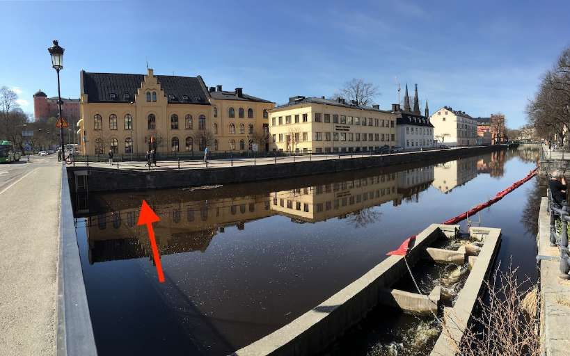
The river reach in the study area is channelised. The section between Islandsfallet
and Kvarnfallet has straight, reinforced sides while the section upstream of Kvarnfallet
has sloped sides lined with trees, reed and other aquatic plants. See Figure A.6 for
representative pictures of different river sections.
The maximum monthly mean potential evaporation in southern Sweden occurs in June
and in 1961-1978 it was 130 mm (B. Eriksson 1981). This gives a maximum evapora-
tion from the Fyris water surface of 0.003 m3 /s. In June, the water flow at Islandsfallet
in 2017 and 2018 was never below 1 m3 /s. In total, this yields the maximum evapora-
tion 3 h of the water flow.
14Upstream of Bärbyleden, the catchment consists of mainly natural rural landscape
agricultural land and forests. There are also an airport, an industrial area and a
smaller urban area with urban runoff outlets at the river just upstream the measur-
ing station at Bärbyleden. Downstream of Bärbyleden, there are several urban runoff
outlets from the separate stormwater sewer system. There are few treatment facilities
such as stormwater ponds or sedimentation chambers in their catchment areas. In ad-
dition to this, the Librobäck tributary joins the Fyris river on the studied river stretch.
The flow from the Librobäck tributary is not continuously measured. However, there
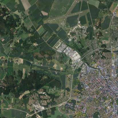
is another small river, the Stabby river, close to the study area, see Figure 8 where
flow is measured continuously. The Librobäck catchment area was delineated using
the free depression flow tool in SCALGO. The Stabby catchment area was obtained
from the Swedish Water Archive (SVAR). The Librobäck catchment area is 26.56 km2
and the Stabby catchment area is 6.18 km2 . The yearly average runoff in the region is
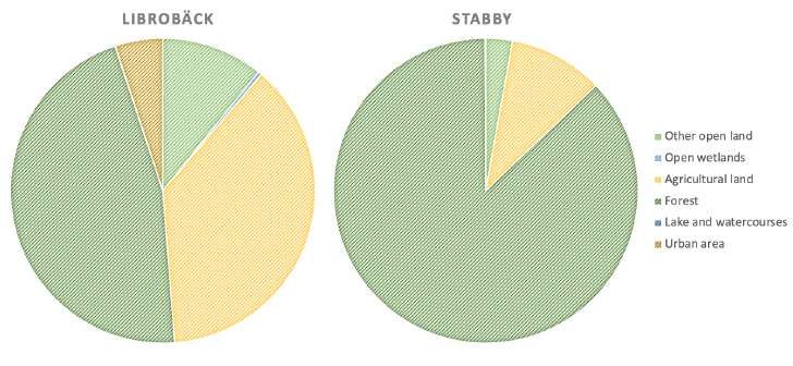
6 - 8 L/s ha (SMHI 2002). The landuse in the Librobäck tributary catchment area is
dominated by agriculture and forest and the Stabby river catchment area is dominated
by forest, see Figure C.3.
Study area
Librobäck
Study area
Librobäck tributary
Stabby river
Stabby
Background: Google Satellite
Figure 8: The study area in red, and the Librobäck catchment area in dotted red line. The Stabby
catchment area, in orange.
The study area is almost exclusively affected by urban runoff while its upstream catch-
ment is predominantly natural land cover. Flanked by two flow measurement stations,
the river stretch makes for a suitable study area, see Figure 6.
In Uppsala, water quality parameters are monitored for the WFD by the Swedish
University of Agricultural Sciences (SLU) (VISS 2019). There is one monitoring station
upstream of the study area at Klastorp, see Figure B.1, and one downstream of the city
(ibid.). The pollutants Pb, Cd and Ni are sampled 12 times a year (ibid.) according
15to a schedule. PAH pollutants are not sampled regularly (VISS 2019).
3.2 Data
Water flow data was obtained from Islandsfallet and Bärbyleden. The measurement
at Islandsfallet is run by the Department of Earth Sciences, Program for Air, Water
and Landscape sciences at Uppsala University in cooperation with the municipality of
Uppsala and Uppsala Vatten (Uppsala University 2021). In summer, a threshold of 20
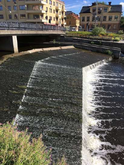
cm is added to the fall, see Figure 9, to ensure a certain water level upstream in the
city, and the data has been corrected for this by Uppsala University (Herbert 2021).
The station measures the water level which can be transformed into flow using a rating
curve (ibid.). Data is recorded hourly (ibid.) and available at http://www.fyris-on-
line.nu/.
(a) Looking upstream. (b) Looking downstream.
Figure 9: Extra threshold added to Islandsfallet in summer. (Photo: Roger Herbert)
The monitoring of the Fyris river at Bärbyleden is run by SMHI. The monitoring
started in 2017 and data is recorded every 15 minutes (Lennermark 2021). The mea-
surement is done using the index technique as there is no deciding section (ibid.), see
Figure 10d. The water level is measured using a ventilated pressure meter which is then
converted to cross-section area (ibid.). Additionally, water velocity below the surface
is measured using hydroacoustics (ADCP), see Figure 10a which is then transformed
to mean water velocity (ibid.). The water flow is then calculated from the area and
the mean water velocity (ibid.). Both the velocity measurement and the cross-sectiona
area are continuously controlled and adjusted (ibid.), see Figure 10b and 10c.
16(a) The hydroacoustic velocity meter submerged. (b) Adjusting cross-section area.
(c) Controlling index station with ADCP boat. (d) Looking downstream towards the index station.
Figure 10: The index station at Bärbyleden. (Photo: Mikael Lennermark)
A map of the technical catchment area in Uppsala was provided by WRS (Öckerman
2021), see Figure 6. It is based on Uppsala Vatten’s stormwater pipe network and
landuse types and it was used to delineate the study area.
Precipitation and air temperature data was obtained from SMHI (SMHI 2021b). Pre-
cipitation data was also obtained from Uppsala Vatten. The SMHI precipitation data
is quality controlled (ibid.) while the Uppsala Vatten rain data is not quality controlled
and might include substantial errors (Jansson 2021).
Flow data was also obtained from the Stabby river The monitoring of the Stabby river
is run by SMHI. Data is recorded every 15 minutes. The measurement is done using
a V-notch weir of 120° (Blomgren 2021), see Figure 11.
17(a) Looking upstream. (b) Looking downstream.
Figure 11: The V-notch weir used for measuring flow in the Stabby river. (Photo: Karin Blomgren)
3.3 Methods
The method of the project consists of two main parts:
1. Estimating and modelling the proportion of urban runoff in the Fyris river during
rain events.
2. Using the proportion of urban runoff in the Fyris river to estimate momentary
pollution concentrations and evaluating the risk of these exceeding MAC-EQS.
3.3.1 Modelling the proportion of urban runoff
For this project, the availability of data, time limitations and the type of end usage
lead to the choice of a lumped model based on a mass balance of water flow. This
water balance model was made for the studied river stretch between Bärbyleden and
Islandsfallet. Urban runoff was approximated by quickflow, assuming that quickflow
from the urban study area is mostly associated with processes such as overland flow
or pipeflow which deliver mostly ’young’ water to the recipient.
The previously introduced surface water system, see Figure 3, was adjusted to accom-
modate for an urban setting with a high occurrence of impervious surfaces and and
a conventional stormwater sewer system, see Figure 12. Slow soil water throughflow
and overland flow were removed. Flow from tributaries and urban runoff baseflow,
which also includes continuous industrial water discharge to the stormwater system,
were added. Rapid soil water throughflow and overland flow were removed. Urban
runoff quickflow caused by rain was added. Flooding is not included since the river
is channelised and have high river banks, which makes flooding very rare. Also, the
complexity of flow and pollution during flooding was not sought to be modelled within
the boundaries of this project. Drinking water outtake and treated wastewater outlet
were added as well as water added during lowflow periods to maintain a certain water
level.
18Figure 12: The hydrological process considered for the water balance in this project. The blue
watercourse can be visually represented as a bucket with inflows (arrows pointing to the watercourse)
and outflows (arrows pointing away from the watercourse).
All the flows in Figure 12 were considered for this project. Drinking water outtake
and lowflow addition occur upstream of the selected study area (Beal 2021) and were
therefore removed from the model. The wastewater treatment plant has its outlet
downstream of the study area and removed as well. The maximum evaporation in
the study area is negligible in comparison to the minimum flow at Islandsfallet so the
evaporation was omitted. Because the city is located on top of a layer of relatively
impermeable clay (Sidenvall 1970) and because the Fyris river is located on the valley
bottom (which is typically a discharge area), the groundwater leakage from the river is
thought to be low and was omitted too. For the hydrograph separation, groundwater
flow and urban runoff baseflow were idealised as continuous baseflow components. The
tributary Librobäck can contribute to quickflow from rainfall of high intensity or big
volume but it will not contribute with water of urban runoff quality. It was therefore
treated separatly to urban runoff quickflow. Lastly, direct channel precipitation could
contribute to quickflow volume, especially at high rain intensities. Rain water contains
fewer pollutants than urban runoff and was therefore treated separatly to urban runoff
quickflow. Hence, the hydrological processes in Figure 12 were simplified into the
water balance model for this project, see Figure 13.
19Figure 13: The water balance model in this project.The blue watercourse can be visually represented
as a bucket with inflows (arrows pointing to the watercourse) and outflows (arrows pointing away
from the watercourse). Qin is the flow at Bärbyleden and Qout is the flow at Islandsfallet.
Rain measurements from several raingauges were first intended to be spatially dis-
tributed over the study area using Thiessen polygons, see Figure 14, in order to obtain
representative data for the studied area. This was deemed an appropriate method
considering the data availability and the flat topography of the study area. However,
when analysing the rain data, discrepancies in the Uppsala Vatten rain data were
found. Moreover, the data differed considerably to data obtained from the SMHI rain
gauges. For example there were long periods without precipitation in the Uppsala
Vatten data. To avoid uncertainties, and to align with the method used in an other
master thesis carried out simultaneously, only the SMHI measurements from Geocen-
trum were used, the station near the Department of Geosciences, Uppsala University.
The Geocentrum station was selected as it was located closest to the study area and
to Islandsfallet of the two SMHI stations.
20Study area
Librobäck tributary
Fyris river
Rain gauges
Uppsala airport (SMHI)
Årsta (UV)
Flogsta (UV)
Geocentrum (SMHI)
Gränby (UV)
Kungsängsverket (UV)
Librobäck (UV)
Background: OpenStreetMap
Figure 14: The rain gauges close to the study area with their corresponding Thiessen polygons. The
rain gauges are run by Uppsala Vatten (UV) and SMHI.
In the first round of selection, potential rain events were identified with the criteria
of a minimum total rain depth of 2 mm and a minimum of 6 h with no precipitation
data between events. If there was a 5 hour gap, or less, in between precipitation, it
was still considered to be the same event. Furthermore, rain events were identified to
occur when the air temperature was above 0 °C and when the unheated raingauges
at Librobäck and Årsta were recording rainfall. Events that did not fulfil the above
criteria were removed as they are possibly snowfall or snowmelt events.
Out of the 232 rain events that were identified, a second selection was done. The
heaviest rains were chosen for further analyse because they were thought to incite
detectable quickflow in the hydrograph, and produce the biggest proportion of urban
runoff in the river. Therefore, based on the qualities of the 232 rain events, only rain
events with a minimum total rain depth of 10 mm and a minimum maximum intensity
of 3 mm/h were kept. 33 such rain events were identified. These will hereinafter be
referred to as the rain events.
The urban runoff quickflow was estimated in several steps according to the water bal-
ance model, Figure 13. These steps are explained in the following paragraphs. To begin
with, the flow contributed from the study area (QStudyarea ) was obtained by subtract-
ing the flow at Bärbyleden (QBärbyleden ) from the flow at Islandsfallet (QIslandsf allet ),
see Equation 4. This was done by adding a time delay (tdelay ) to the flow at Bärbyle-
den, corresponding to the rising limb at Bärbyleden to reach Islandsfallet. The time
delay was set individually for each year. The time delay was needed as the lumped
model omits the transport processes within the "bucket". Any inflow or outflow should
be perceived as instantaneous regardless of the actual access point. The time delay
was selected through ocular trial and error of overlaying the flow curves. According
to the water balance, Figure 13, this leaves the baseflow, tributary flow and chan-
21You can also read