Philadelphia Water Department Watershed Protection Program - Delaware Estuary Salinity Model Validation May 2020

Philadelphia Water
 Department
 Watershed Protection
 Program

 Delaware Estuary
 Salinity Model Validation

 May 2020

Philadelphia Water Department May 2020

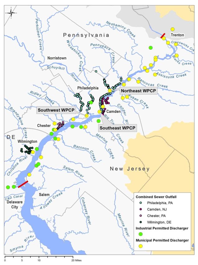
Table of Contents
1.0 Introduction .................................................................................................................................... 1
2.0 Numerical Model ........................................................................................................................... 1
 2.1 Model Objectives ........................................................................................................................ 1
 2.2 Modeling Approach................................................................................................................... 1
 2.3 Study Area .................................................................................................................................. 3
 2.4 Salinity Conversion Methods ................................................................................................... 5
 2.5 Boundary Conditions ................................................................................................................ 5
 2.5.1 Tributaries ........................................................................................................................... 5
 2.5.2 Open Boundary Condition -Salinity.............................................................................. 18
 2.5.3 CSOs ................................................................................................................................... 25
 2.5.4 Withdrawals and Discharges in the Model Domain ................................................... 29
 2.5.5 Boundary Conditions Summary .................................................................................... 37
 2.6 Initial Conditions ..................................................................................................................... 40
 2.6.1 Temperature...................................................................................................................... 40
 2.6.2 Salinity ............................................................................................................................... 40
 2.7 Grid and Bathymetry ............................................................................................................... 40
3.0 Sensitivity Studies ........................................................................................................................ 42
 3.1 Bottom Roughness ................................................................................................................... 43
 3.2 Turbulent diffusion and turbulence closure settings .......................................................... 45
 3.3 Open Boundary Loading ........................................................................................................ 47
 3.3.1 Loading adjustment for stratification ............................................................................ 47
 3.3.2 Mixed vs stratified input ................................................................................................. 49
 3.4 Grid Adjustment ...................................................................................................................... 50
 3.4.1 Fine vs. coarse grid .......................................................................................................... 50
 3.5 Tributary loading ..................................................................................................................... 52
 3.5.1 Tributary Flow Estimates ................................................................................................ 52
 3.5.2 Final adjustment of generated tributary salt loads...................................................... 54
 3.6 Salt load analysis ...................................................................................................................... 55
4.0 Salinity Model Validation ........................................................................................................... 56
 4.1 Validation configuration - 2014.............................................................................................. 56
 4.1.1 River Discharges............................................................................................................... 57

Philadelphia Water Department May 2020

4.1.2 Water Level ....................................................................................................................... 57
 4.1.3 Salinity ............................................................................................................................... 57
 4.1.4 Wind................................................................................................................................... 57
 4.1.5 Grid and bottom roughness............................................................................................ 57
 4.2 Validation Metrics .................................................................................................................... 58
 4.2.1 Mean Error, RMSE and Skill Factor ............................................................................... 58
 4.2.2 Tidal Analysis Method .................................................................................................... 59
 4.3 Validation Results .................................................................................................................... 59
 4.3.1 Hydrodynamics ................................................................................................................ 59
 4.3.2 Salinity ............................................................................................................................... 65
5.0 Conclusions and Summary ......................................................................................................... 71
6.0 References ..................................................................................................................................... 72

Philadelphia Water Department May 2020

List of Tables
Table 2-1: Summary Salinity Modeling Approach Sources ................................................................. 2
Table 2-2: Tributaries included in model domain ................................................................................. 7
Table 2-3: Observed tributary specific conductance data availability and gap filling
methodology for 2014 & 2016 ................................................................................................................. 10
Table 2-4: Median grab sample salinity [PSU] for ungaged tributaries. Spr: Spring (3/1 - 6/15),
Sum: Summer (6/16 - 9/30), Win: Winter (10/1 - 2/28), D: Dry, W: Wet ....................................... 13
Table 2-5: Vertical adjustment factors for ungaged Tributaries ........................................................ 17
Table 2-6: Salinity time series for tributaries without salinity related data ..................................... 18
Table 2-7: Regression Results ................................................................................................................. 24
Table 2-8: Adjustment factors for 2014 and 2016 ................................................................................. 25
Table 2-9: Discharge Only Facilities Included in PWD Salinity Model ............................................ 32
Table 2-10: Withdrawals Included in PWD Salinity Model ............................................................... 35
Table 2-11: Consumptive Use of Withdrawals and Discharges ........................................................ 36
Table 2-12: Return Flow Facilities .......................................................................................................... 37
Table 2-13: Summary of chloride distribution from model discharge inputs excluding the ocean
end open boundary.................................................................................................................................. 38
Table 2-14: Summary of chloride distribution from model discharge inputs excluding the ocean
end open boundary.................................................................................................................................. 39
Table 3-1: Model grid metrics ................................................................................................................. 50
Table 3-2: Flow Reduction Targets ........................................................................................................ 54
Table 4-1: EFDC model settings ............................................................................................................. 57
Table 4-2: Modeled Water Level Mean Error, RMSE and Skill Factor ............................................. 59
Table 4-3: Water Level Tidal Analysis for 2014. Validation period of 9/1 – 11/30. ....................... 60
Table 4-4: Water Level Tidal Analysis for 2016. Validation period of 4/1 – 6/30. ......................... 61
Table 4-5: Modeled Velocity Mean Error, RMSE and Skill Factor .................................................... 62
Table 4-6: Current Tidal Analysis for 2014. Validation period of 9/1 – 11/30. .............................. 63
Table 4-7: Current Tidal Analysis for 2016. Validation period of 4/1 – 6/30. ................................ 64
Table 4-8: Salinity validation metrics in PSU and mg/L chloride .................................................... 65

Philadelphia Water Department May 2020

List of Figures
Figure 2-1: Map of Delaware Estuary with along-channel river mile reference locations .............. 4
Figure 2-2: Tributary and River Monitoring .......................................................................................... 6
Figure 2-3: Salinity at Brandywine, Wissahickon and Cobbs Creeks ............................................... 10
Figure 2-4: Seasonal identification of wet weather threshold, Neshaminy Creek example .......... 12
Figure 2-5: Similar range – Assiscunk grab sample vs. Brandywine ................................................ 14
Figure 2-6: Dissimilar range – Crosswicks grab sample vs. Brandywine ........................................ 15
Figure 2-7: Neshaminy vs. Pennypack .................................................................................................. 15
Figure 2-8: Generated Raccoon Creek Salinity vs. Brandywine Creek Salinity .............................. 16
Figure 2-9: Amplitude of specific conductivity for tidal constituents: 2014 and 2016 at Reedy
Island Jetty (RIJ) and Pea Patch Island (PPI) ........................................................................................ 20
Figure 2-10: Phase of Specific Conductivity for Tidal Constituents: 2014 and 2016....................... 21
Figure 2-11: Permitted Discharges and Combined Sewer Outfalls .................................................. 28
Figure 2-12: Summary of chloride distribution from model discharge inputs as a percent
excluding the ocean end open boundary.............................................................................................. 38
Figure 2-13: Summary of streamflow distribution from model inputs as a percent excluding the
ocean end open boundary ...................................................................................................................... 39
Figure 2-14: Model fine grid ................................................................................................................... 41
Figure 3-1: Validated roughness distribution ...................................................................................... 44
Figure 3-2: Original COA vs. adjusted bottom roughness – Buoy C. Maximum bottom to
surface salinity difference is 1.08 psu for adjusted roughness case and 0.30 psu for original case.
 .................................................................................................................................................................... 45
Figure 3-3: Original vs. adjusted bottom roughness – Buoy B .......................................................... 45
Figure 3-4: Buoy C – default turbulence closure setting vs. alternate setting of CTE3=5.0.
Maximum bottom to surface salinity difference is 1.08 psu for alternate case and 0.39 psu for
default case at Buoy C. ............................................................................................................................ 46
Figure 3-5: Buoy B – default turbulence closure setting vs. alternate setting of CTE3=5.0. .......... 47
Figure 3-6: Observed salinity 2014 (orange) and 2016 (blue) at Buoy P ........................................... 47
Figure 3-7: Along Channel Salinity Survey 2011 (Aristizábal & Chant, 2014) ................................ 48
Figure 3-8: Buoy C – Lower Boundary Salinity x 1.0 (LBCx1.0) vs Salinity x 1.2 (LBCx1.2) ......... 48
Figure 3-9: Buoy B – Lower Boundary Salinity x 1.0 (LBCx1.0) vs Salinity x 1.2 (LBCx1.2) ......... 49
Figure 3-10: Buoy C - mixed vs stratified salinity boundary condition. Maximum bottom to
surface salinity difference is 1.18 psu for mixed case and 1.05 psu for stratified case. .................. 49
Figure 3-11: Buoy B - mixed vs stratified salinity boundary condition ............................................ 50
Figure 3-12: Subtidal model results for along channel velocity at Buoy C for Fine Grid (upper)
and Coarse Grid (lower) show improved match to observations for fine grid as opposed to
coarse grid. Surface and bottom labels refer to mean of top two and bottom two layers
respectively. .............................................................................................................................................. 51
Figure 3-13: Subtidal model results for salinity [PSU] at Buoy B show improved match to
observations for fine grid as opposed to the coarse grid ................................................................... 52
Figure 3-14: Subtidal model results for salinity [PSU] at Ben Franklin Bridge (lower) show
improved match to observations for fine grid as opposed to the coarse grid................................. 52
Figure 3-15: Salinity at Buoy B original flow estimate vs. reduced flow ......................................... 53
Figure 3-16: Salinity at Ben Franklin Bridge original flow estimate vs. reduced flow ................... 53

Philadelphia Water Department May 2020

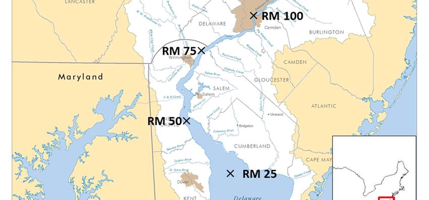
Figure 3-17: Salinity at Baxter – original vs. adjusted tributary salinity estimates vs. observed .. 55
Figure 4-1: Low-passed current comparison for bottom and surface layers, 2014. ........................ 64
Figure 4-2: 2014 (upper) and 2016 (lower) low-passed salinity at Buoy C, validation period 9/1 –
10/26. ......................................................................................................................................................... 66
Figure 4-3: 2014 (upper) and 2016 (lower) low-passed salinity at Chester, validation period 9/1–
10/26. ......................................................................................................................................................... 67
Figure 4-4: 2014 (upper) and 2016 (lower) low-passed salinity at Buoy B, validation period 9/1 –
10/26. Maxima for modeled and observed salinity show that model captures presence of salt
longitudinally. .......................................................................................................................................... 68
Figure 4-5: 2014 (upper) and 2016 (lower) low-passed salinity at Ben Franklin Bridge, validation
period 9/1 – 10/26. .................................................................................................................................. 69
Figure 4-6: Low-passed salinity at Baxter, validation period 9/1 – 10/26. ..................................... 70

Philadelphia Water Department May 2020

Acronyms
 Acronym Description
 ADCP Acoustic Doppler Current Profiler
 C&D Canal Chesapeake and Delaware Canal
 CFS Cubic Feet Per Second
 CSO Combined Sewage Overflow
 CTD Conductivity, Temperature, Depth sensor
 DRBC Delaware River Basin Commission
 EFDC Environmental Fluid Dynamics Code
 EMC Event Mean Concentrations
 EPA US Environmental Protection Agency
 LBC Lower Boundary Condition
 MGD Million Gallons per Day
 NPDES National Pollutant Discharge Elimination System
 PWD Philadelphia Water Department
 RMSE Root Mean Square Error
 SIPS Strain-induced Periodic Stratification
 TDS Total Dissolved Solids
 USGS United States Geological Survey
 NOAA National Oceanic and Atmospheric Administration
 PSU Practical Salinity Unit

Philadelphia Water Department May 2020

1.0 Introduction
The Philadelphia Water Department (PWD) Water Quality Compliance Modeling (WQCM)
group within the Watershed Protection Program performs modeling and analysis of water
quality in the tidal Delaware River, which is the source for 60% of the drinking water to the City
of Philadelphia. To support infrastructure planning for the PWD Baxter Water Treatment Plant,
the PWD estuarine salinity model was developed to enhance the understanding of how salinity
intrusion and sea level rise may influence drinking source water quality. The tidal Delaware
River is a high quality source of drinking water to the City of Philadelphia, and also a source for
process and cooling water to many industries and manufacturers. During severe droughts the
tidal Delaware River adjacent to Philadelphia experiences salinity intrusion, during which
ocean salt is transported further upstream then during normal conditions.
The current conditions that lead to salinity intrusion as well as the conditions that can manage
salinity intrusion will be explored with the PWD salinity model. This report details the
components of the PWD salinity model, calibration steps and model validation.
This report does not include the additional model setup necessary to simulate sea level rise.
Further work is required to approximate the influence that sea level rise may have on model
setup and assumptions related to bathymetry and morphology changes, salinity and boundary
conditions. Following the completion of salt line analyses of current conditions with this
validated model, PWD will work to amend the model inputs and assumptions to perform sea
level rise analyses. PWD will issue an Appendix to this validation report at that time
documenting all model changes and assumptions related to sea level rise analysis.

2.0 Numerical Model
2.1 Model Objectives
The objective of the model development is to create a salinity model that can simulate salinity
conditions in the tidal upper Delaware Estuary, specifically in the region adjacent the City of
Philadelphia and the PWD Samuel S. Baxter Water Treatment Plant (Baxter). Model predictions
are compared to observed conditions at stations in the Delaware River to calibrate and validate
the model. For this report, salinity conditions for the years 2014 (main validation) and 2016
(drought conditions in fall) are simulated, with special concentration on analyzing axial salt
distributions during low flow periods in late summer and early fall. Sensitivity analyses are
performed with respect to salt transport and hydrodynamic conditions to better understand and
replicate important physical processes.

2.2 Modeling Approach
Various sources that contribute salt to the tidal Delaware River considered here include:
 Marine salt transported from the Delaware Bay
 Land-based sources delivered by tributary rivers and creeks
 Land-based sources delivered by stormwater runoff
 Process-water sources discharged directly to tidal waters

Section 2: Numerical Model Page 1

Philadelphia Water Department May 2020

The complexity of salt transport in tidal waters suggested the need for a 3-dimensional
hydrodynamic and transport modeling approach and the US Environmental Protection Agency
(EPA) Environmental Fluid Dynamics Code (EFDC) was selected for this application. Table 2-1
summarizes input sources and model parameters for the modeling approach used to develop
the PWD salinity model, the major elements of which are described below and throughout this
report.
Table 2-1: Summary Salinity Modeling Approach Sources
 System Inputs Sources Parameters
 Tributaries and Direct Runoff National Pollution Discharge
 Elimination System (NPDES)
  USGS gaging stations and CTD sensors
 Permitted Dischargers, Tributaries,
 Philadelphia Combined Sewer Overflows
 and Direct Runoff
 (CSOs)
  Flow Rate
  Direct Combined Sewer System
  Temperature
 Stormwater Management Model (SWMM)
  Salinity from specific
  CSOs discharging into Non-tidal Cobbs
 conductance/total dissolved
 and Tookany Tacony-Frankford Creeks
 Loads solids
 above U.S. Geologic Survey (USGS) gaging
 stations were represented by USGS gaging
 stations and CTD sensors
 Camden County Municipal Authority,
 Delaware County, Delaware County Regional
 Authority, and Wilmington CSOs
  Estimates based on available information
 Permitted Dischargers
  Discharge Monitoring Reports (DMRs)
  National Oceanic and Atmospheric  Water Level
 Downstream Open Administration (NOAA) tide and  Temperature
 Boundary (Lower temperature gage at Delaware City, DE  Salinity from specific conductance
 Model Extent)  PWD conductivity, temperature and depth
 (CTD) sensor
  NOAA National Climatic Data Center  Wind Speed and Direction
 (NCDC) Station at the Philadelphia  Air Temperature
 Climate International Airport  Dew Point Temperature
  Algorithms for Clear-Sky Solar Radiation  Atmospheric Pressure
  Cloud Cover and Solar Radiation
  Friction Height
 Hydrodynamic  Turbulence closure
 Model  Salt transport
  Temperature

Section 2: Numerical Model Page 2

Philadelphia Water Department May 2020

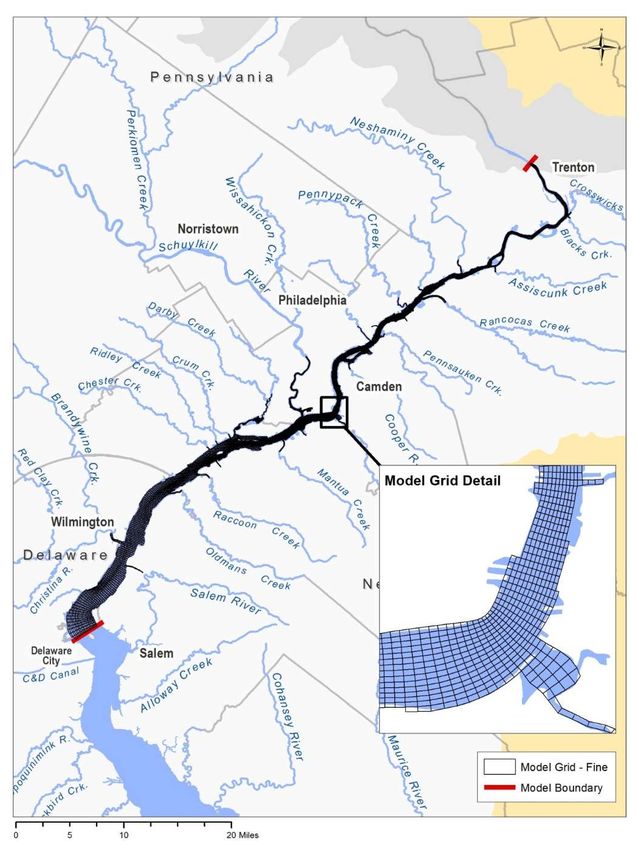
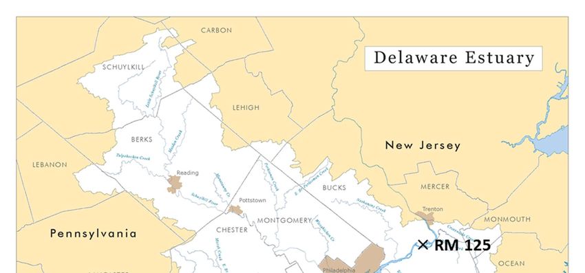
2.3 Study Area
The principal sources of freshwater discharge to the Delaware Estuary is the Delaware River at
the head of tide at Trenton, New Jersey, supplying about 52% of the total mean freshwater
inflow (Ketchum, 1953; Garvine, McCarthy and Wong, 1992). Between the head of tide, and
Delaware City, DE, the Schuylkill River and 41 other tributaries contribute additional
freshwater to the upper estuarine system. The domain of this study includes the tidal
freshwater region, including tidal reaches from 3 miles above the confluence with the
Chesapeake and Delaware Canal to the head of tide at Trenton, stretching from River Mile 61.8
to 134.4 (Note that the DRBC River Mile system is used throughout this report; see:
https://www.nj.gov/drbc/basin/river/ ).
The Delaware Bay is a weakly stratified coastal plain estuary (Janzen and Wong, 2002). The
principal interface between the predominantly freshwater portions and the saltier waters of the
lower Bay generally is located between River Miles 31 and 75. Salt transport in this part of the
Delaware Estuary is predominantly driven by gravitational circulation with strong
contributions from secondary lateral flow (Aristizábal and Chant, 2015). Philadelphia County is
situated between River Mile 91 and River Mile 111, upstream of the average landward extent of
marine salt intrusion (Figure 2-1).
Hydrodynamics and transport in the upper estuary are driven primarily by the interactions of
nonlinearities among tidal flows, freshwater inputs, gravitational circulation, and
meteorological influences (Garvine, McCarthy and Wong, 1992). Secondary driving
mechanisms may include the effects of axial curvature and Ekman forcing (Chant, 2009), and
the action of vertical shear flow dispersion (Linden and Simpson, 1986; Garvine, McCarthy and
Wong, 1992). Analysis of current data at River Mile 75 suggests the existence of vertical shear
flow dispersion through strain-induced periodic stratification (SIPS) (Simpson et.al., 1990)
during low flow/high salinity intrusion events, usually in late summer/fall. As well, analysis
of cross channel currents at this location suggest that differential advection may contribute to
estuarine circulation (Lercak & Geyer, 2004; Macready & Geyer, 2010). Together these
mechanisms may contribute to enhanced upstream transport of marine salt in the lower domain
of the model during periods of low freshwater inflow.

Section 2: Numerical Model Page 3

Philadelphia Water Department May 2020

Figure 2-1: Map of Delaware Estuary with along-channel river mile reference locations

Section 2: Numerical Model Page 4

Philadelphia Water Department May 2020

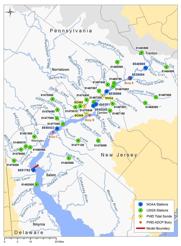
2.4 Salinity Conversion Methods
The EFDC model needs salt related boundary and initial conditions as salinity in Practical
Salinity Unit (PSU). The data used for the model inputs comes from a variety of sources, in
different formats and units, thus conversion methods are required. Most continuous data
sources, such as tributary sondes, allow estimates of salt content from observations of specific
conductance [S/cm] and associated water temperatures (degrees C). Tributary grab samples
and industrial or municipal discharges report salt also in measures of chloride and Total
Dissolved Solids (TDS) in mg per liter. Specific Conductivity and temperature may be used to
estimate salinity. Standard Methods 2520 B and D provide background, references, and
calculations for estimating salinity through conductance and temperature observed in natural
waters. When salinity is determined through conductivity measurements it is based on the
Practical Salinity Scale.
For chloride, a relationship to salinity is developed based on available paired data from
combined PWD and DRBC Boat Run data. Observed specific conductance and temperature
values from this dataset are converted to salinity using the above method and analyzed with
paired chloride values using a combination of MATLAB’s POLYFIT, POLYCONF, and
CORRCOEF functions to create a linear regression equation with the 95% confidence interval
and the Pearson’s R-squared coefficient. The resulting equations are below.
S = CL*1.8e-03 + 0.046 (Eq. 2-1)
S = TDS*8.5e-04+0.052 (Eq. 2-2)

2.5 Boundary Conditions
Boundary conditions for the 2014 and 2o16 salinity models include discharge, salinity and
temperature for tributaries and anthropogenic point sources, such as stormwater Combined
Sewer Overflows (CSOs), municipal and industrial dischargers, salinity, water temperature and
water level at the open boundary, and atmospheric and wind information.

2.5.1 Tributaries
2.5.1.1 Streamflow
Streamflow is monitored by United States Geological Survey (USGS) at stations on many of the
rivers and creeks within the Delaware River watershed. Records of continuous streamflow time
series are available from USGS for most of the major tributary rivers and creeks of the tidal
Delaware River within the model domain from Trenton to Delaware City (Figure 2-2).
Streamflow estimates for ungaged tributaries are prepared using a watershed area ratio method
with flow data from nearby or similar gaged tributaries. The USGS stations on the gaged
tributaries are located on the streams above the influence of the tide. For many of the
tributaries, especially on the New Jersey side of the Delaware River where the watershed is
relatively flat, a significant portion of the watersheds lie downstream of the gage.

Section 2: Numerical Model Page 5

Philadelphia Water Department May 2020

Figure 2-2: Tributary and River Monitoring
Section 2: Numerical Model Page 6

Philadelphia Water Department May 2020

The watershed area ratio method is used to estimate streamflow from these lower (ungaged)
watershed areas based on the flow recorded at the USGS gage of the tributary. Flow is also
estimated using the watershed area ratio method for the areas between tributaries that
contribute stormwater runoff directly to the Delaware River. These areas are referred to as
“direct runoff areas.” During the salinity model validation, it is determined to be necessary to
make some adjustments to the flows estimated for the ungaged tributaries and direct runoff
areas. This process is discussed in further detail in Section 3.5.
Gaps larger than 6 hours in the gaged tributary streamflow data are filled using the average
daily discharge reported by USGS when data points are missing during peak flow events. Gaps
in streamflow during essentially constant baseflow conditions are linearly interpolated by the
model itself. Table 2-2 provides an overview of the tributaries that are included in the model
domain with information on gage availability and gap filling.
Table 2-2: Tributaries included in model domain

 USGS River
 River/Tributary Gap Filling or Ungaged Estimate Methodology
 Gage Mile
 2014: 8 gaps filled w/ daily avg. discharge
Delaware River 01463500 134.25
 2016: 7 gaps filled w/ daily avg. discharge
Blacks Creek None Crosswicks Creek 128.0
Crosswicks Creek 01464500 Only 2014: 4 gaps filled w/ daily avg. discharge 128.0
Stream @ Crystal
 None Crosswicks Creek 126.0
Lake
Crafts Creek None Crosswicks Creek 124.0
Bustleton Creek None Crosswicks Creek 119.75
Assiscunk Creek None Rancocas Creek 118.0
Stream @
 None Rancocas Creek 117.75
Burlington
 2014: 4 gaps filled w/ daily avg. discharge
Neshaminy Creek 01465500 115.0
 2016: 6 gaps filled w/ daily avg. discharge
Poquessing Creek 01465798 Only 2016: 3 gaps filled w/ daily avg. discharge 111.25
Swede Run None Cooper River 110.75
Rancocas Creek
 01467000 NA 110.5
north
Rancocas Creek
 01465850 Only 2014: 5 gaps filled w/ daily avg. discharge 110.5
south
Pennypack Creek 01467048 Only 2016: 3 gaps filled w/ daily avg. discharge 109.0
Pompeston Creek None Cooper River 108.5
Pennsauken Creek 01467081 Only 2016: 1 gap filled w/ daily avg. discharge 104.75
Frankford Creek 01467087 Only 2014: 3 gaps filled w/ daily avg. discharge 104.0
Cooper River 01467150 Only 2014: 1 gap filled w/ daily avg. discharge 100.5
Newton Creek None Cooper River 96.75

Section 2: Numerical Model Page 7

Philadelphia Water Department May 2020

USGS River
 River/Tributary Gap Filling or Ungaged Estimate Methodology
 Gage Mile
Big Timber Creek None Cooper River 95.5
Schuylkill River 01474500 Only 2014: 1 gap filled w/ daily avg. discharge 92.25
Woodbury Creek None Cooper River 91.5
Little Mantua Creek None Mantua Creek 90.5
Mantua Creek 01475000 Raccoon Creek, Salem River 89.75
Clonmell Creek None Mantua Creek 87.0
 2014: 5 gaps filled w/ daily avg. discharge
Cobbs Creek 01475548 85.0
 2016: 2 gaps filled w/ daily avg. discharge
Darby Creek None Crum Creek 85.0
 2014: 7 gaps filled w/ daily avg. discharge
Crum Creek 01475850 84.8
 2016: 2 gaps filled w/ daily avg. discharge
 2014: 7 gaps filled w/ daily avg. discharge
Ridley Creek 01476480 84.0
 2016: 5 gaps filled w/ daily avg. discharge
 2014: 5 gaps filled w/ daily avg. discharge
Chester Creek 01477000 82.5
 2016: 4 gaps filled w/ daily avg. discharge
Little Timber Creek None Raccoon Creek 82.5
Still Run None Raccoon Creek 82.0
 2014: 8 gaps filled w/ daily avg. discharge
Raccoon Creek 01477120 80.0
 2016: 3 gaps filled w/ daily avg. discharge
Stoney Creek None Chester Creek 80.0
Marcus Hook Creek None Chester Creek 79.5
Namaan Creek None Chester Creek 77.75
Oldmans Creek None Raccoon Creek 76.0
 2014: 4 gaps filled w/ daily avg. discharge
Brandywine River 01481500 70.5
 2016: 2 gaps filled w/ daily avg. discharge
Christina River 01478000 Only 2016: 34 gaps filled w/ daily avg. discharge 70.5
 2014: 6 gaps filled w/ daily avg. discharge
Red Clay Creek 01480015 70.5
 2016: 5 gaps filled w/ daily avg. discharge
 2014: 6 gaps filled w/ daily avg. discharge
White Clay Creek 01479000 70.5
 2016: 5 gaps filled w/ daily avg. discharge
 2014: 2 gaps filled w/ daily avg. discharge
Salem River 01482500 68.75
 2016: Raccoon Creek
Army Creek None Christina River 64.0

2.5.1.2 Salinity for Gaged Tributaries
Temperature, used together with salinity for calculating density in the hydrodynamic model, is
available for several tributaries and can also be used as substitutes for ungaged tributaries
because of temperature’s low spatial variability. However, continuous specific conductance
time series are only available for very few tributaries. An approach was needed to generate
Section 2: Numerical Model Page 8

Philadelphia Water Department May 2020

continuous specific conductance time series for all tributaries based on available data. In
addition to the few time series that were available, grab samples are used to determine median
values for ungaged tributaries.
Continuous specific conductance data from USGS gages is available at the Delaware River at
Trenton (USGS01463500), Schuylkill River at Philadelphia (USGS01474500), and Brandywine
Creek (USGS01481500). Data for Christina River is ignored because it is influenced by salinity
from downstream due to tides. USGS data from PWD maintained stations is available at
Poquessing Creek, Pennypack Creek, Frankford Creek, and Cobbs Creek.
Potential specific conductance data for gap filling from upstream USGS gages is available at
Schuylkill River at Norristown, Pennypack Creek at Pine Road, Tacony Creek at Adams Ave,
Schuylkill at Philadelphia, and Cobbs Creek at Highway 1.
Reference specific conductance data in the Delaware River main stem for calibration/validation
is available at Delaware River at Chester, PA (USGS01477050), Delaware River at Ben Franklin
Bridge (USGS01467200), Delaware River at Pennypack Woods (USGS014670261), PWD Buoy B
at Eagle Point and Buoy C at Marcus Hook.
An overview of available specific conductance data periods, gaps, and data used for gap filling
can be found in Table 2-3 below and their respective locations in Figure 2-2.
In a first check, missing data entries marked as NaN (Not a Number) are removed from each
time series. The remaining time series is checked for gap longer than one day. Only gaps from
stations with data that exhibited large amplitudes or that missed salinity events in winter are
gap filled. Gaps during dry weather or with small amplitude data, such as in the main stem
salinity stations, can be considered constant conditions and are left untreated to be linearly
interpolated directly by the model. Occasional outliers are adjusted manually to better-match
ambient conditions as seen in the measurements directly before and after the outlier.
Most tributary-specific conductance stations do not operate in winter due to potential ice
damage. The only continuous tributary time series that covered the full year is available for
Brandywine Creek. Time periods in early and late winter that showed data for both
Brandywine and those tributaries without winter data are used to determine a multiplication
adjustment factor and vertical shift for Brandywine data, to match the receiving waters time
series.

Section 2: Numerical Model Page 9

Philadelphia Water Department May 2020

Table 2-3: Observed tributary specific conductance data availability and gap filling methodology for
2014 & 2016

 Delaware
 USGS
 River/Tributary Gap Filling Methodology River
 Gage
 Mile
 2014: No missing data 134.25
Delaware 01481500
 2016: No missing data
Delaware River @ 2014: Winter gap filled w/ shifted Baxter 100.00
 01467200 2016: No missing data
Ben Franklin Bridge
Schuylkill @ 2014: Winter gap filled w/ Queen Lane Schuylkill
 01474500
Fairmount Dam 2016: Winter gap filled w/ shifted Belmont
Delaware River @ 2014: No missing data 82.50
 01477000
Chester 2016: Winter gap filled w/ shifted Baxter
 2014: No missing data 70.50
Brandywine 01481500
 2016: No missing data
 2014: Winter gap filled w/ shifted Wissahickon 111.25
Poquessing (PWD) 01465798
 2016: Winter gap filled w/ shifted Wissahickon
 2014: 2 gaps about a day long; 1 gap is 4 days long 110.50
Baxter (PWD) 014670261
 2016: 1st gap filled w/ shifted Brandywine
 2014: Winter gap filled w/ shifted Wissahickon 109.00
Pennypack (PWD) 01467048
 2016: Winter gap filled w/ Poquessing
 2014: Winter gap filled w/ shifted Pennypack 104.00
Frankford (PWD) 01467087 2016: Winter gap filled w/ shifted Pennypack
 2014: Winter gap filled w/ shifted Brandywine Schuylkill
Wissahickon (PWD) 01474000
 2016: Winter gap filled w/ shifted Brandywine
 2014: Winter gap filled w/ shifted Wissahickon 2016: 85.00
Cobbs (PWD) 01475548
 Winter gap filled w/ shifted Wissahickon

The urban tributaries typically exhibit distinctly different temporal patterns than Brandywine
Creek. Overall, they are higher in salinity and show larger dilution excursions during wet
weather events. Figure 2-3 shows the salinity time series at Brandywine (light grey),
Wissahickon (dark grey), and Cobbs (black), which is similar to Frankford and Pennypack
Creeks.

Figure 2-3: Salinity at Brandywine, Wissahickon and Cobbs Creeks
Section 2: Numerical Model Page 10

Philadelphia Water Department May 2020

The offset is clearly visible and shows that Wissahickon is the most complete time series with
only a one month-long winter gap at the beginning of 2014. This gap was filled with
Brandywine data. In 2016 a Wissahickon winter gap at the beginning, and another at the end of
the year, were filled with Brandywine data. Gap-filled Wissahickon data is then used to fill the
winter gaps of Poquessing, Pennypack and Cobbs Creeks.
Depending on the original time step, all final time series are interpolated onto a regularly
spaced time vector to assure that discharge and salinity boundary time series are on the same
time-step. This facilitates an easier calculation of model factoids (such as load etc.) for future
meta data purposes. Delaware River specific conductance is recorded on an hourly time step,
Schuylkill River, Baxter and Poquessing Creek on 30 minutes, and all other stations on 15
minutes.
2.5.1.3 Synthesized Salinity Time Series for Ungaged Tributaries
Long term grab sample data for salt content is available for several tributaries in the model
domain. Data was analyzed for median values and presented in Table 2-4 below. Depending on
data availability and sensitivity to seasons and precipitation, medians are determined for
yearly, seasonal or seasonal-wet/dry conditions to support estimates of salinity in ungaged
tributaries.
To assemble artificial time series for ungaged tributaries, estimates of their average salinity are
needed. All available USGS parameters (salinity [PSU], specific conductance [S/cm], chloride
(CL) [mg/l], and TDS [mg/l]) per tributary are first collected and analyzed. Conversion
methods from these parameters to salinity [PSU] are detailed in Section 2.4.
For all gaged rivers, flow thresholds for wet/dry conditions are determined using a cumulative
distribution function (CDF) plot. Figure 2-4 shows CDF plots for biological Spring, Summer
and Winter, with cumulative probability on the x-axis and discharge in cms on the y-axis. The
blue line is the graphed CDF. The method analyzes each flow time series of all available years
bound by the dates of each biological season, which are respectively plotted as a cumulative
distribution function for each local tributary. The value at which the function deviates from this
linear relationship is selected as the wet-weather threshold, with any flow values above this
threshold yielding a wet-weather identification. To limit the frequency of false positives,
roughly 5% of the max flow is added as a buffer.
Comparison of the threshold to the discharge at grab sample time in the river (or a river nearby,
if fully ungaged) helped to determine if the sample was taken during wet or dry weather
conditions which has an influence on the salinity. In summer, rain events usually dilute the
river water, leading to lower salinity spikes, and in winter snow is often connected to a spike in
salinity because of the use of road salts, which eventually wash off streets and into nearby rivers
directly or by drainage systems.

Section 2: Numerical Model Page 11

Philadelphia Water Department May 2020

Spring (3/1 - 6/15), Summer (6/16 - 9/30), Winter (10/1 - 2/28)
Figure 2-4: Seasonal identification of wet weather threshold, Neshaminy Creek example
Additionally, the season in which the sample was taken is determined. Using this information,
plots by tributary for seasons, flow (wet/dry), and wet/dry seasons for all salinity related
parameters are generated and respective median values determined (Table 2-4).
While some tributaries showed a sensitivity to wet/dry events, most can be described by a
constant salinity value, either by season or yearly. The final seasonal and overall ungaged
tributary salinity is presented in Table 2-4 below. Biological seasons are defined as Spr: Spring
(3/1 - 6/15), Sum: Summer (6/16 - 9/30), Win: Winter (10/1 - 2/28)

Section 2: Numerical Model Page 12

Philadelphia Water Department May 2020

Table 2-4: Median grab sample salinity [PSU] for ungaged tributaries. Spr: Spring (3/1 - 6/15), Sum:
Summer (6/16 - 9/30), Win: Winter (10/1 - 2/28), D: Dry, W: Wet

 Tributary Approach Spr Sum Win SpD SpW SuD SuW WiD WiW Overall
 Assiscunk overall 0.11
 Assunpink seasons 0.13 0.15 0.16
 Army seasons 0.19 0.12 0.14
 Blacks overall 0.09
 Big Timber seasons 0.08 0.08 0.09
 Crafts overall 0.14
 Crosswicks seasons 0.08 0.10 0.09
 Chester overall 0.20
 Crum overall 0.12
 Cooper seasons 0.14 0.10 0.10
 seasons/
 Doctors 0.08 0.08 0.10 0.08 0.10 0.10
 weather
 Not enough
 Mantua data, use donor
 trib
 seasons/
 Naaman 0.19 0.18 0.17 0.16 0.15 0.19
 weather
 seasons/
 Neshaminy 0.20 0.22 0.25 0.20 0.26 0.24
 weather
 Newton overall 0.12
 Oldmans seasons 0.09 0.10 0.11
 Pennsauke
 seasons 0.14 0.12 0.14
 n
 RancocasN overall 0.02
 RancocasS overall 0.09
 Raccoon seasons 0.10 0.10 0.11
 Red Clay overall 0.19
 Ridley overall 0.15
 Shellpot seasons 0.25 0.21 0.24
 Still Run overall 0.11
 Salem seasons 0.12 0.12 0.13
 Swede Run overall 0.15
 Not enough
 Woodbury data, use donor
 trib
 White Clay overall 0.17
 flow weighted
 Ranocas mean North & 0.06
 South branch

Section 2: Numerical Model Page 13

Philadelphia Water Department May 2020

Tributary discharge time series can be used to determine when a dilution event caused by
precipitation happens. It is more difficult to predict when a spike in salinity from snow, ice and
road salt is going to happen, because such events are not necessarily reflected in the streamflow
record. Therefore, it was decided to generate a yearly time series with two procedures. For this
the year was split into winter (01/01-03/15 and 12/01-12/31) and non-winter periods (03/16-
11/30), times when it is assumed to snow and freeze, or rain. For the non-winter period, the
respective medians are assigned, using a related discharge time series to determine wet events
if applicable. For winter, Brandywine or gap filled Pennypack time series are used, with slight
adjustments to ensure a smooth transition to the respective non-winter data.
Long-term grab sample data showed that all tributaries, except for Neshaminy Creek,
resembled Brandywine Creek. In Figure 2-5 to Figure 2-7, long term continuous Brandywine
salinity is plotted against the respective grab samples of the tributaries.

Figure 2-5: Similar range – Assiscunk grab sample vs. Brandywine
Grab sample data measured as chloride (CL), specific conductance (SC), and total dissolved
solids (TDS) are converted to salinity (Sal) using the methods described in Section 2.4 (denoted
as CL2Sal, SC2Sal, and TDS2Sal in the figures). Many are on the same order as Brandywine
Creek salinity (such as Assiscunk Creek Figure 2-5) or a little below (e.g. Crosswicks Creek
Figure 2-6).

Section 2: Numerical Model Page 14

Philadelphia Water Department May 2020

Figure 2-6: Dissimilar range – Crosswicks grab sample vs. Brandywine
Neshaminy Creek resembles the higher salinity regime of Pennypack and other Philadelphia
Creeks (Figure 2-7). There is insufficient data to compare higher peak values in winter to grab
sample data, which are seldom taken during or right after respective peak salinity events.
Therefore, it was decided to only apply a vertical shift to the Brandywine time series that brings
base salinity to the same level as suggested in the grab sample data.

Figure 2-7: Neshaminy vs. Pennypack

Section 2: Numerical Model Page 15

Philadelphia Water Department May 2020

A last check of the method is made when connecting the median-based and Brandywine time series
together into one (Figure 2-8). If Brandywine connects smoothly to the following median time series, no
adjustment is needed. In some cases, slight adjustments are made to the vertical factor to improve the
transition (Table 2-5).

Figure 2-8: Generated Raccoon Creek Salinity vs. Brandywine Creek Salinity

Section 2: Numerical Model Page 16

Philadelphia Water Department May 2020

Table 2-5: Vertical adjustment factors for ungaged Tributaries

 Vertical adjustment Tributary for winter
 Tributary
 factor [PSU] gap
 Assiscunk Creek -0.03 Brandywine Creek
 Assunpink Creek 0 Brandywine Creek
 Army Creek 0 Brandywine Creek
 Blacks Creek -0.05 Brandywine Creek
 Big Timber Creek -0.05 Brandywine Creek
 Crafts Creek 0 Brandywine Creek
 Crosswicks Creek -0.05 Brandywine Creek
 Chester Creek 0.05 Brandywine Creek
 Crum Creek -0.02 Brandywine Creek
 Cooper River 0 Brandywine Creek
 Mantua Creek -0.04 Brandywine Creek
 Namaan Creek 0.05 Brandywine Creek
 Neshaminy Creek 0 Pennypack Creek
 Newton Creek -0.02 Brandywine Creek
 Oldmans Creek -0.05 Brandywine Creek
 Pennsauken Creek 0 Brandywine Creek
 Rancocas Creek -0.09 Brandywine Creek
 Raccoon Creek -0.04 Brandywine Creek
 Red Clay Creek 0.03 Brandywine Creek
 Ridley Creek 0.02 Brandywine Creek
 Shellpot Creek 0 Brandywine Creek
 Still Run -0.03 Brandywine Creek
 Salem River -0.02 Brandywine Creek
 Swede Run 0.01 Brandywine Creek
 Woodbury Creek -0.04 Brandywine Creek
 White Clay Creek 0.03 Brandywine Creek

Time series are created for all tributaries with grab sample data using this method. For a few
remaining tributaries for which no data exists, the salinity time series of a nearby tributary are
used (Table 2-6).

Section 2: Numerical Model Page 17

Philadelphia Water Department May 2020

Table 2-6: Salinity time series for tributaries without salinity related data

 Tributary Without Data Supplemental Tributary Used
 Burlington Assiscunk Creek
 Bustleton Creek Crafts Creek
 Clonmell Creek Still Run
 Crystal Lake Crafts Creek
 Darby Creek Cobbs Creek
 Little Mantua Creek Big Timber Creek
 Little Timber Creek Big Timber Creek
 Mantua Creek Big Timber Creek
 Marcus Hook Creek Crum Creek
 Pompeston Creek Swede Run
 Woodbury Creek Big Timber Creek

2.5.2 Open Boundary Condition -Salinity
Specific Conductivity data for the near surface waters was collected for PWD by the Woods
Hole Group in the vicinity of Pea Patch Island (PPI) during the spring, summer and fall of both
2014 and 2016. The purpose of this data collection effort was to inform the ocean-end member
salinity boundary condition for the PWD EFDC modeling efforts. To develop annual series of
continuous salinity concentrations for all of 2014 and 2016 without gaps, relationships are
developed between the observed data collected at Pea Patch Island, and the data collected by
USGS at Reedy Island Jetty (RIJ) in 2014 and 2016. Time series analyses and multivariate
statistical modeling are performed to develop the relationships that are used to fill the data
gaps.
The observed data from Pea Patch island are transformed to average hourly specific
conductivity estimates for use in these analyses, for the periods:
May 8, 2014 – October 26, 2014: 4,128 continuous hours;
April 5, 2016 – October 16, 2016: 4,680 continuous hours.
Data for the Reedy Island Jetty station are retrieved from the USGS National Water Information
System web interface (Delaware River at Reedy Island Jetty, DE – 01482800) in an hourly
format, and converted to Eastern Standard Time for the period:
September 1, 2007 23:00 hrs. – January 5, 2017 10:00 hrs., 79,382 hours
Minor gaps exist in the 2014 (3 hours) and 2016 (5 hours) Reedy Island Jetty record for periods
when the PWD Pea Patch island data acquisition system was not active. These gaps are filled
using linear interpretation estimates.

Section 2: Numerical Model Page 18

Philadelphia Water Department May 2020

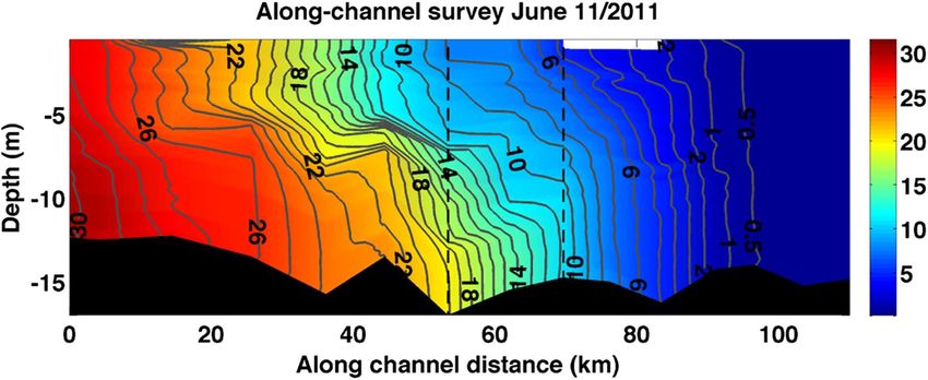
2.5.2.1 Synthesizing a Continuous Estimate of Specific Conductivity at Pea
 Patch Island
The axial salinity distribution in an estuary results from the relative proportions of sea water
and upland runoff from the head of tide, as mixed by tidal and meteorological conditions. The
salinity distribution in the Delaware Estuary and its relationships to fresh water inflow have
been explored by many investigators (see Rosensweig, 1940; Ketchum, 1951; Cohen and
McCarthy, 1962; Sharp, et.al, 1983, Garvine, McCarthy and Wong, 1992; Wong, 1995). Most
have concluded that the along-estuary distribution of salinity in the estuary is predominantly
the result of tidal mixing, upon which is superimposed on a weak river flow, which essentially
is Stommel’s original concept that was published in 1951. This concept especially is applicable
in the domain of the PWD EFDC model, where essentially there is no vertical salinity
stratification (or at most, only ephemeral, weak stratification, mostly limited to the lower
portions of the model domain). A recent observational study of the mid-Delaware Bay
(Aristizábal & Chant, 2014) found that lateral circulation played a dominant role in enhancing
tidally varying stratification.
Initially some effort was expended in this investigation to relate various measures of fresh
water inflow to the hourly Specific Conductivity both at Pea Patch Island and at Reedy Island
Jetty. Specifically, the subtidal Specific Conductivity signals were compared to numerous
lagged accumulations of Delaware River inflow at Trenton and Schuylkill River inflow at
Philadelphia. In addition, effects of the implied transport through the Chesapeake and
Delaware Canal was included in that analysis. In general, the relationships investigated
consistently explained no more than about 50%-60% of the variance in Specific Conductivity,
with the most favorable lag of about 3 weeks from the time of the Trenton daily discharge. That
result is consistent with expectations that measures of fresh water inflow alone cannot be
expected to fully describe salinity conditions along the estuary, especially when employing only
multivariate statistical tools in the time domain.
The early work on fresh water discharge - conductivity response reinforced a return to
exploring the relationships between the Specific Conductivity signal at Reedy Island Jetty and
the signal at Pea Patch Island to yield a reliable predictive capability for the EFDC model
boundary condition. The concept is that the net fresh water inflow and large-scale tidal and
meteorological influences predominantly are reflected in the Specific Conductivity at subtidal
frequencies. The readily available continuous Specific Conductivity data reliably recorded by
USGS at Reedy Island Jetty at sub-hourly time steps makes it attractive to use as an exogenous
input to predict values at Pea Patch Island.
2.5.2.2 Comparison of the Subtidal Frequencies Signals
A time series of hourly subtidal (low-passed) Specific Conductivity is estimated by applying a
modified Lanczos filter with a cutoff period of 34 hours and a filter length with a half-window-
width of 1.5 times the cut-off period, yielding an hourly filter length of 109 weights. Inspection
of the time series graphs of these low-passed results for Reedy Island Jetty and Pea Patch Island
revealed that the subtidal Specific Conductivity at the two stations appear well correlated and
in phase with one another for the periods of concurrent observations in both 2014 and 2016.

Section 2: Numerical Model Page 19

Philadelphia Water Department May 2020

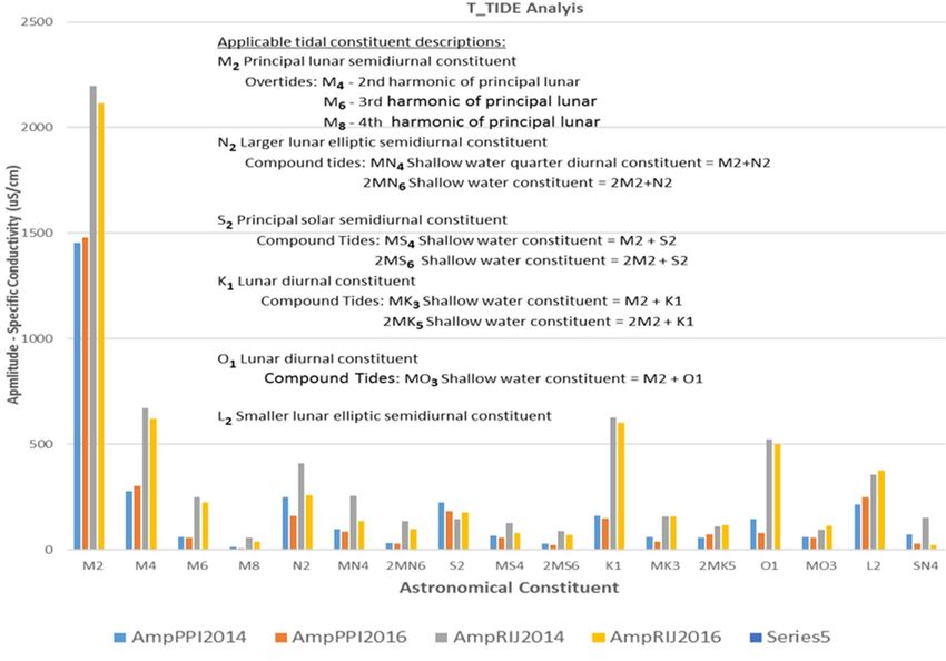
2.5.2.3 Comparison of the Tidal Frequencies Signals
The tidal frequency signals are estimated by subtracting the low-passed time series from the
hourly time series, attributing the resultant residual time series to the tidal (and super-tidal)
signal. This tidal residual information was further scrutinized for astronomically-driven
harmonic responses by analyzing the time series using the T_TIDES software, applied in Octave
(Pawlowicz, Beardsley and Lentz, 2002). The tidal harmonic analysis is performed for each
station for each year individually, for the period of overlap when the Pea Patch Island station
was active in 2014 (141 days(1)) and 2016 (195 days). The results for the 17 tidal constituents that
exhibited the largest amplitudes and the highest signal-to-noise ratios in the T_TIDE results are
shown in Figure 2-9 below (S/N generally > 3, with 3 cases > 1.5; M8 was allowed in for Pea
Patch Island 2016 for completeness, even though the S/N was 0.67).

Figure 2-9: Amplitude of specific conductivity for tidal constituents: 2014 and 2016 at Reedy Island
Jetty (RIJ) and Pea Patch Island (PPI)

(1)Note that the data acquired before early June of 2014 was not used in this analysis because the
high volume of river inflow associated with the Spring freshet during that period caused the
tidal-frequency signal sinusoidal pattern at Pea Patch Island to be clipped. For valid results, the
harmonic analysis (T_TIDE) software expects full range sinusoids, i.e., a random, ergodic
stationary sinusoidal signal.
Section 2: Numerical Model Page 20

Philadelphia Water Department May 2020

The results of the tidal harmonic analysis indicate that the relationships of tidal-frequency
amplitude between the two monitoring periods are quite similar for each station. While in
general the amplitudes of the Specific Conductivity signal for each constituent at Pea Patch
Island are damped relative to that at Reedy Island Jetty (which is assumed to be attributable to
the location of Pea Patch Island further upstream, closer to the principal sources of fresh water
runoff), they fairly consistently exhibit similar constituent-to-constituent patterns in amplitude.
In addition, the differences in phase for the tidal constituents between Pea Patch Island and
Reedy Island Jetty (phases are shown in Figure 2-10 below) generally are quite small for the
principal constituents that actually are the result of a celestial motion (i.e., M2, N2, S2, K1, O1 and
L2). For instance, the M2 constituent phase at Reedy Island Jetty only differs from the phase at
Pea Patch Island by a few degrees. The only primary constituent with a large station-to-station
and year-to-year variance was N2, but on closer inspection the amplitude is small and that is the
only constituent with large phase errors reported by T_TIDE, in fact the phase error exceeded
the values of the phase. But overall for the principal constituents, the signals are similar in their
respective response to whatever forcings are driving them at tidal frequencies, demonstrating
that the Reedy Island data makes a reasonably good surrogate for the Pea Patch Island signal at
tidal frequencies.

 350

 300

 250
Phase - Specific Conductivity

 200
 (Degrees)

 150

 100

 50

 0
 M2 M4 M6 M8 N2 MN4 2MN6 S2 MS4 2MS6 K1 MK3 2MK5 O1 MO3 L2
 Astronomical Constituent
 PhasePPI14 PhasePPI16 PhaseRIJ14 PhaseRIJ16

Figure 2-10: Phase of Specific Conductivity for Tidal Constituents: 2014 and 2016

Section 2: Numerical Model Page 21

Philadelphia Water Department May 2020

2.5.2.4 Developing a Predictive Equation - Estimating Specific Conductivity at
 Pea Patch Island from Reedy Island Data
As discussed previously, preliminary work led to the result that all subsequent modeling would
be performed on a two-variate basis, decomposing the times series of Specific Conductivity into
a subtidal (low-pass filtered) signal and, by subtraction, a residual signal that includes tidal
frequencies. The subtidal signal was estimated by applying a modified Lanczos filter as
described above. The tidal-frequencies signal was created by subtracting the low-passed
filtered signal from the original time series, essentially creating a high-passed series that
includes the tidal-frequencies and any higher frequencies.
2.5.2.5 Preliminary Investigations Seeking a Predictive Equation
Initially, a series of regression analyses were performed, first with the low-passed, subtidal-
frequency hourly Specific Conductivity series at Buoy P, versus the subtidal-frequency hourly
Specific Conductivity series at Reedy Island Jetty, and then with the addition of residual-
frequency (high-passed, tidal frequencies and greater) hourly Specific Conductivity at Buoy P
versus the residual-frequency hourly Specific Conductivity at Reedy Island Jetty. These
regressions were performed on the 2014 data, with the 2016 data used for validation. Initial
indications from this work was encouraging, with the low-passed signal at Reedy Island Jetty
explaining about 90% of the variance of the low-passed signal at Buoy P/Pea Patch Island in
2016, and the high-passed signal from Reedy Island Jetty explaining about 50% or more of the
residual high-passed signal at Pea Patch Island in 2016. The predictions for the total signal at
Pea Patch Island for 2016 yielded root mean square errors in the range of 900-1,000 S/cm (0.4-
0.5 ppt salinity).
When the T_TIDE analyses were performed on the two tidal-frequency series, it admitted the
opportunity to use the harmonics-predictive capabilities of T_TIDE to provide an input-output
model for the tidal frequency signals. That line of investigation was explored, but the resulting
root mean square error estimates increased over those yielded by the preliminary regression
work, typically by about an additional 500 S/cm or more. An important underpinning of the
harmonic analysis approach is that the time series is stationary in a statistical sense, and there
are no temporal modal fluctuations in the mean, and no non-tidal trends in the data. Scrutiny
of the graphical results readily revealed that a harmonic prediction approach loses the ability to
reflect modal changes in Specific Conductivity that, one assumes, is a result of forcings such as
changes in fresh water flow or other meteorological factors, and mixing dynamics, that were not
removed by the filter. It is not unreasonable to assume that the reason such relatively short-
duration modal shifts can remain in the high-passed filtered tidal-frequencies may belie the
inherent numerical inefficiency of the filter to eliminate all the energy from the near-tidal
periods (filter “leakage” around the cut-off, 24-72-hours). When these ephemeral fluctuations
appear in the record, they cannot be reproduced by a harmonic analysis approach. However,
the regression analysis approach readily accommodates directly linearly transferring such
fluctuations from the Reedy Island Jetty to the Pea Patch Island output signal. Therefore, a
regression approach is favored.

Section 2: Numerical Model Page 22

Philadelphia Water Department May 2020