Timely prediction potential of landslide early warning systems with multispectral remote sensing: a conceptual approach tested in the Sattelkar ...
←
→
Page content transcription
If your browser does not render page correctly, please read the page content below
Timely prediction potential of landslide early warning systems with
     multispectral remote sensing: a conceptual approach tested in the
     Sattelkar, Austria
     Doris Hermle1, Markus Keuschnig2, Ingo Hartmeyer2, Robert Delleske2 and Michael Krautblatter1
     1
 5   Technical University of Munich, Chair of Landslide Research, Munich, Germany
     2
     GEORESEARCH Forschungsgesellschaft mbH, Puch, Austria
     Correspondence to: Doris Hermle (doris.hermle@tum.de)

     Abstract
     While optical remote sensing has demonstrated its capabilities for landslide detection and monitoring, spatial and temporal
10   demands for landslide early warning systems (LEWS) were not met until recently. We introduce a novel conceptual
     approach to structure and quantitatively assess lead time for LEWS. We analysed “time to warning” as a sequence; (i) time
     to collect, (ii) to process and (iii) to evaluate relevant optical data. The difference between “time to warning” and
     “forecasting window” (i.e. time from hazard becoming predictable until event) is the lead time for reactive measures. We
     tested digital image correlation (DIC) of best–suited spatiotemporal techniques, i.e. 3 m resolution PlanetScope daily
15   imagery, and 0.16 m resolution UAS derived orthophotos to reveal fast ground displacement and acceleration of a deep–
     seated, complex alpine mass movement leading to massive debris flow events. The time to warning for UAS and
     PlanetScope totals 31h/21h and is comprised of (i) time to collect 12/14h, (ii) process 17/5h and (iii) evaluate 2/2h, which is
     well below the forecasting window for recent benchmarks and facilitates lead time for reactive measures. We show optical
     remote sensing data can support LEWS with a sufficiently fast processing time, demonstrating the feasibility of optical
20   sensors for LEWS.

     1 Introduction

     Landslides are a major natural hazard leading to human casualties and socio–economic impacts, mainly by causing
     infrastructure damage (Dikau et al., 1996; Hilker et al., 2009). They are often triggered by earthquakes, intense short–period
     or prolonged precipitation, and human activities (Hungr et al., 2014; Froude and Petley, 2018). In a systematic review
25   Gariano and Guzzetti (2016) report that 80 % of the papers examined show causal relationships between landslides and
     climate change. The ongoing warming of the climate (IPCC, 2014) is likely to decrease slope stability and increase landslide
     activity (Huggel et al., 2012; Seneviratne et al., 2012), which indicates a vital need to improve the ability to detect, monitor
     and issue early warnings of landslides and thus to reduce and mitigate landslide risk.
     Early warning, refers to a set of capacities for the timely and effective provision of warning information through institutions,
30   such that individuals, communities and organisations exposed to a hazard are able to take action with sufficient time to
     reduce or avoid risk and prepare an effective response (UNISDR, 2009). According to UNISDR (2006), an effective early
     warning system consists of four elements: (1) risk knowledge, the systematic data collection and risk assessment; (2) the
     monitoring and warning service; (3) the dissemination and communication of risk as well as early warnings; and (4) the
     response capabilities on local and national levels. Lead time as defined in the context of LEWS is the interval between the
35   issue of a warning (i.e. dissemination) and the forecasted landslide onset (Pecoraro et al. 2019) and thus crucially depends on
     time requirements in phases (1)–(3). The success of an EWS therefore requires measurable pre–failure motion (or slow slope
     displacement) to allow for sufficient lead time for decisions on reactions and counter measures (Grasso, 2014; Hungr et al.,
     2014).

                                                                    1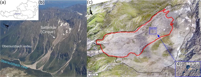
While remote sensing has been established for early warnings, remote sensing is not yet used for real early warnings of the
40   onset of landslides in steep–alpine terrain (with a few exceptions), where geotechnical instruments are still preferred.
     Exceptions include terrestrial InSAR (Pesci et al., 2011; Walter et al. 2020) and terrestrial laser scanning with high repetition
     rates. However, repeated UAS (unmanned aerial systems) and optical satellite images (PlanetScope) with high repetition
     rates have so far not been applied for landslide early warning in steep-alpine catchments. In this regard, knowledge of sensor
     capabilities and limitations is essential, as it determines which rates and magnitudes of pre-failure motion can potentially be
45   identified (Desrues et al., 2019). Our proposed framework refers to mass movements in steep–alpine catchments with
     significant pre–failure motion over sufficient time periods and thus excludes instantaneous events triggered by processes
     such as heavy rainfalls or earthquakes.
     This study presents a new concept to systematically evaluate remote sensing techniques to estimate and increase lead time
     for landslide early warnings in these catchments. We do not start from the perspective of available data; instead, we define
50   necessary time constraints to successfully employ remote–sensing data to provide early warnings. This approach reduces to a
     small number the suitable remote sensing products with high temporal and spatial resolution. With these constraints, we
     investigated the application of data from satellites and UAS to allow the assessment of the data, after a spaceborne area–wide
     but low–resolution acquisition, into a downscaled detailed image recording. In so doing, we analysed the capability of these
     different passive remote sensing systems focusing on spatiotemporal capabilities for ground motion detection and landslide
55   evolution to provide early warnings.

     Recently, the spatial and temporal resolution of optical satellite imagery has significantly improved (Scaioni et al., 2014) and
     has allowed substantial advances in the definition of displacement rates and acceleration thresholds to approach requirements
     for early warning purposes. This is essential since spatial and temporal resolution determine whether landslide monitoring is
60   possible with the detection of displacement rates and approximate acceleration thresholds, both of which are lacking if
     information is based solely on post–event studies (Reid et al., 2008; Calvello, 2017). Landslide monitoring offers the
     potential to significantly advance landslide early warning systems (LEWS) (Chae et al., 2017; Crosta et al., 2017).
     Previously, high spatial resolution satellite data was obtained at the expense of a reduction in the revisit rates (Aubrecht et
     al., 2017). Consequently, the return period between two images increased, limiting ground displacement assessment and the
65   range of observable motion rates. The number of useful images was further reduced due to natural factors such as snow
     cover, cloud cover and cloud shadows. High–resolution remote sensing data was long restricted due to high costs and data
     volume (Goodchild, 2011; Westoby et al., 2012). Today commercial very high resolution (VHR) optical satellites exist, but
     tasked acquisitions make them inflexible and very cost intensive, thus limiting research (Butler, 2014; Lucieer et al., 2014).
     There is a vast spectrum of available remote sensing data with high spatiotemporal resolution (Table 1). Complementary use
70   of different remote sensing sources can significantly improve landslide assessment as demonstrated by Stumpf et al. (2018)
     and Bontemps et al. (2018), who draw on archive data and utilise different sensor combinations to analyse the evolution of
     ground motion.

     Table 1 Overview of different optical multispectral remote sensors with their corresponding resolution [m] and revisit rate [days]. The
75   sensors are categorised into commercial and free data policy. 1free quota via Planet Labs Education and Research Program, 2PlanetScope
     Ortho Scene Product, Level 3B/Ortho Tile Product, Level 3A (Planet Labs, 2020b), 3reached end of life, 3/2020, archive data usable, 45 m
     Ortho Tile Level 3A (Planet Labs, 2020a), 50.5 m colour pansharpened, 6self–acquired. Source: (ESA, 2020).

         Sensor         Temporal        Spatial            Free/
                      resolution [d] resolution [m]      Commercial
     UAS                     flexible         0.08               F6
     WorldView 2                  1.1         1.84               C
     WorldView 3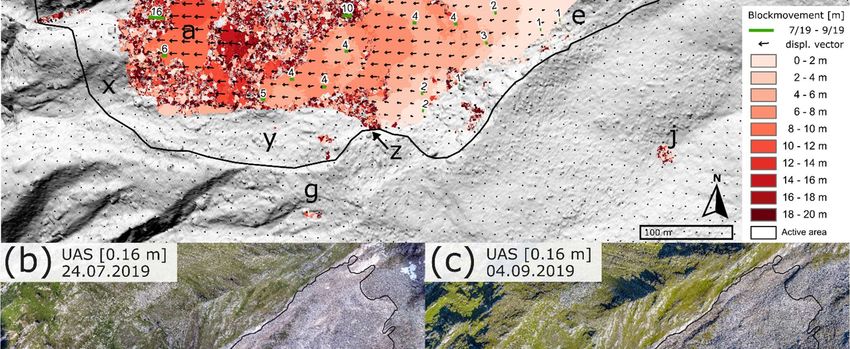
GeoEye–1                      3          1.64              C
      Pléiades 1A/B                 1     2.0 (0.5)5             C
      PlanetScope                   1    3.0/3.1252            C/F1
      RapidEye3                   5.5             54              F
      Sentinel–2 A/B                5            10               F
      Landsat 8                   16             30               F

 80   The latest developments in earth observation programs include both the new Copernicus’ Sentinel fleet operated by the ESA,
      and a new generation of micro cube satellites, sent into orbit in large numbers by PlanetLabs Inc. These micro cube
      satellites, known as 'Doves'/PlanetScope (from now on referred to as PlanetScope satellites), and Sentinel–2 a/b offer very
      high revisit rates of 1–5 days and high spatial resolutions from 3–10 m, respectively (Table 1), for multispectral imagery
      (Drusch et al., 2012; Butler, 2014; Breger, 2017). These high spatiotemporal resolutions open up unprecedented possibilities
 85   to study a wide range of landslide velocities and natural hazards through remote sensing. Continuing data access is fostered
      by PlanetLabs and by Copernicus (via its open data policy) providing affordable or free data for research. Examples of
      landslide activity studies employing multi–temporal datasets based on this access to high spatiotemporal data include
      Lacroix et al. (2018), using Sentinel–2 scenes to detect motions of the 'Harmalière' landslide in France, and Mazzanti et al.
      (2020), who applied a large stack of PlanetScope images for the active Rattlesnake landslide, USA.
 90   As landslides tend to accelerate beyond the deformation rate observable with radar systems before failure, we concentrate on
      optical image analysis (Moretto et al., 2016). One advantage of optical imagery is its temporally dense data (Table 1)
      compared to open data radar systems with sensor repeat frequency every six days and revisit frequency between three days at
      the equator, about two days over Europe and less than one day at high latitudes (Sentinel–1, ESA). Optical data allows direct
      visual impressions from the multispectral representation of the acquisition target and the option to employ this data for
 95   further complementary and expert analyses. While active radar systems overcome constraints posed by clouds and do not
      require daylight, data voids can be significant due to layover or shadowing effects in steep mountainous areas (Mazzanti et
      al., 2012; Plank et al., 2015; Moretto et al., 2016). Moreover, north/south facing slopes are less suitable, thus limit the range
      of investigation (Darvishi et al., 2018). In general, sensor choice depends on the landslide motion rate with radar at the lower
      and optical instruments at the upper motion range (Crosetto et al., 2016; Moretto et al., 2017; Lacroix et al., 2019).
100   However, a flexible, cost–effective alternative to spaceborne optical data are airborne optical images taken by UASs. Freely
      selectable flight routes and acquisition dates enable avoiding shadows from clouds and topographic obstacles as well as
      unfavourable weather conditions and summer time snow cover, all of which frequently impair satellite images (Giordan et
      al., 2018; Lucieer et al., 2014). UAS–based surveys provide accurate very high resolution (few cm) orthoimages and digital
      elevation models (DEM) of relatively small areas, suitable for detailed, repeated analyses and geomorphological applications
105   (Westoby et al., 2012; Turner et al., 2015).
      In recent years, data provision for users has increased and today data hubs provide easy accessibility to rapid, pre–processed
      imagery. Nonetheless, technological advances can be misleading as they promise high spatiotemporal data availability,
      which frequently does not reflect reality (Sudmanns et al., 2019). One key problem is the realistic net temporal data
      resolution which is often significantly reduced due to technical issues, such as image errors and non–existent data (i.e. data
110   availability, completeness, reliability). Other problems include data quality and accuracy in terms of geometric, radiometric
      and spectral factors (Batini et al., 2017; Barsi et al., 2018). Knowledge of the most useful remote sensing data options is vital
      for complex, time–critical analyses such as ground motion monitoring and landslide early warning. Timely information
      extraction and interpretation are critical for landslide early warnings yet few studies have so far explicitly focused on time
      criticality and the influence of the net temporal resolution of remote sensing data.
115   In this investigation we propose both a conceptual approach to evaluating lead time as a time difference between the “time to
      predict” and the “forecasting time” and assess the suitability of UAS sensors (0.16 m) and PlanetScope (3 m) imagery (the
      latter with temporal proximity to the UAS acquisition) for LEWS. For this we have chosen the 'Sattelkar', a steep, high–

                                                                      3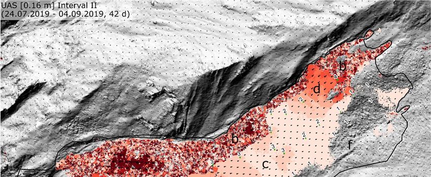
alpine cirque located in the Hohe Tauern Range, Austria (Anker et al., 2016). We estimate times for the three steps (i)
      collecting images, (ii) pre–processing and motion derivation by digital image correlation (DIC) and (iii) evaluating and
120   visualizing. The results from the Sattelkar site – and from historic landslide events – will be discussed in terms of usability
      and processing duration for critical data source selection which directly influences the forecasting window. Accordingly, we
      try to answer the following research questions:
          1.   How can we evaluate lead time as a time difference between the “time to predict” and the forecasting time for high
               spatiotemporal resolution sensors?
125       2.   How can we quantify “time to warning” as a sequence of (i) time to collect, (ii) to process and (iii) to evaluate
               relevant optical data?
          3.   How can we practically derive profound “time to warning” estimates as a sequence of (i), (ii) and (iii) from UAS
               and PlanetScope high spatiotemporal resolution sensors?
          4.   Are estimated “times to warning” significantly shorter than the forecasting time for recent well–documented
130            examples and able to generate robust estimations of lead time available to enable reactive measures and evacuation?

      2 Lead time – a conceptual approach

      2.1. The conceptual approach

      Natural processes and their developments constantly take place independently, thus dictate the technical approaches and
      methodologies researchers can and must apply within a certain time period. For that reason, we hypothesise the forecasting
135   window texternal is externally controlled, consequently the applicability of LEWS methods (tinternal) is restricted because they
      must be shorter than texternal. This approach is the framework of our time concept (Fig. 1).

      Figure 1 The novel conceptual approach for lead time, time to warning and the forecasting window for optical image analysis.

                                                                         4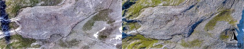
The forecasting window is started (texternal, green dashed outline) following significant acceleration exceeding a set
140   displacement threshold, leading to a continuous process. Simultaneously with the forecasting window, time to warning
      (twarning) starts (grey outline). Time to warning is divided into a three–phase–process to allow time estimations for a
      comparative assessment of different types of remote sensing data. This process consists of the phases (1) time to collect, (2)
      time to process and (3) time to evaluate, each with their individual durations. Confidence in the forecasted event increases
      with time as process acceleration becomes more certain. Once a warning is released (orange box), the lead time begins (tlead)
145   and is terminated by the following release and subsequent impact (red box). The lead time is the difference between the
      forecasting window and the time to warning. During the lead time, reaction time (treact) starts when appropriate counter
      measures are taken to prepare for and reduce risks ahead of the impending event, and ends with the final impact.
      The time to warning period (twarning) is defined by the time necessary to systematically collect data, analyse the available
      information and to evaluate it. Hence, the greater the lead time, the more extensive countermeasures can be implemented
150   prior to the event. An imperative for an effective EWS, the required time to take appropriate mitigation and response
      measures has to be within the lead time interval (tlead) (Pecoraro et al., 2019) with tlead ≥ treact.

      2.2. Practical implementation of multispectral data in the concept

      The time to warning consists of a three–phase–process (see Sect. 2.1. and Fig. 1) to allow rough time estimations for a
      comparative assessment of different types of remote sensing data. Nevertheless, to realise this temporal concept an
155   established, operating system is required, which includes reference data (DEM, previous results), experience from past field
      work and ready UAS flight plans with preparation for a UAS flight campaign, satellite data access, experience in the single
      software processing steps including final classification and visualisation templates and, if utilised for UAS, installed and
      measured ground control points.
      The first phase includes the collection of data starting from the acquisition by the sensor, the data transfer, image pre–
160   processing and provision to the end user. The user selects images online from the data hub, downloads and organises them.
      For a UAS campaign, the user must obtain flight permits, check flight paths and conduct the UAS flight. The second phase
      encompasses time to process for the complete data handling from the downloaded data to final analysis–ready image stacks
      in a GIS or a corresponding software. These preparatory steps may include image selection and renaming, atmospheric
      correction, co–registration, resampling and translation to other spatial resolutions and geographic projection systems,
165   adjustments such as clipping, stacking of single bands into one multispectral image or the division into single bands,
      calculation of hillshade from DEM among others, depending on the requirements. Following this preparation, the data is
      processed with the appropriate software tools to derive ground motion, calculate total displacement and derive surface
      changes, e.g. volume calculations or profiles. In the third and last phase, time to evaluate, the results are compared to
      inventory data and, if available, ground truth data, displacement results of other sensors or different spatial resolutions,
170   different time interval variations to observe changes in sensitivity to meteorological conditions. Additionally, filters may be
      applied to eliminate noise. Finally, the results are analysed and evaluated. In each phase quality management is carried out
      for data access and pre–and post–processing. In time to collect, the images must be selected manually prior to any download
      from the data hub, as its filter tool options on cloud and scene coverage are of limited help. Accordingly, the areal selection
      may be misleading as the region of interest (RoI) might not be fully covered, though the sought–for, smaller area of interest
175   (AoI) is covered but not returned from the request. Concerning cloud filters, first, the filter refers to the RoI as a whole in
      terms of percentage of cloud coverage. The AoI can still be free of clouds or else be the only area covered by clouds in the
      total RoI. Therefore, an image is either not returned although usable, or returned but not useable. Second, clouds can create
      shadows for which no filter is available. As a result, affected images have to be manually removed by the user. Images which
      are of low quality due to snow cover have to be discarded, too. These actions indirectly represent first quality checks in the
180   collection phase. In the following processing phase, the images in a GIS, are checked for quality and accuracy. Depending

                                                                         5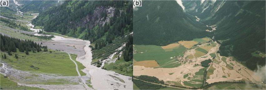
on the data provider, some pre–processing such as radiometric, atmospheric and/or geometric corrections may have been
conducted. During this phase, additional user–based steps will be checked if necessary. Finally, the results are compared to
other data (e.g. DEM, dGPS), reviewed for their validity and may be supplemented by statistical evaluation.
3 Study Site
185 The Sattelkar is a steep, high–alpine, deglaciated west–facing cirque at an altitude of between 2 130–2 730 m asl in the
Obersulzbach valley, Großvenedigergruppe, Austria (Fig. 2a). Surrounded by a headwall of granitic gneiss, the cirque infill
is characterised by massive volumes of glacial and periglacial debris as well as rockfall deposits (Fig. 2b, c). Since 2003
surface changes have taken place as evidenced by a massive degradation of the vegetation cover and the exposure and
increased mobilisation of loose material. A terrain analysis revealed that a deep–seated, retrogressive movement in the debris
190 cover of the cirque had been initiated (Anker et al., 2016; GeoResearch, 2018). High water (over)saturation is assumed to be
causing the spreading and sliding of the glacial and periglacial debris cover on the underlying, glacially smoothed bedrock
cirque floor forming a complex landslide (Hungr et al., 2014). Detailed aerial orthophoto analyses, witness reports and
damage documentations indicate a steady increase in mass movement and debris flow activity over the last decade (Anker et
al., 2016).
195
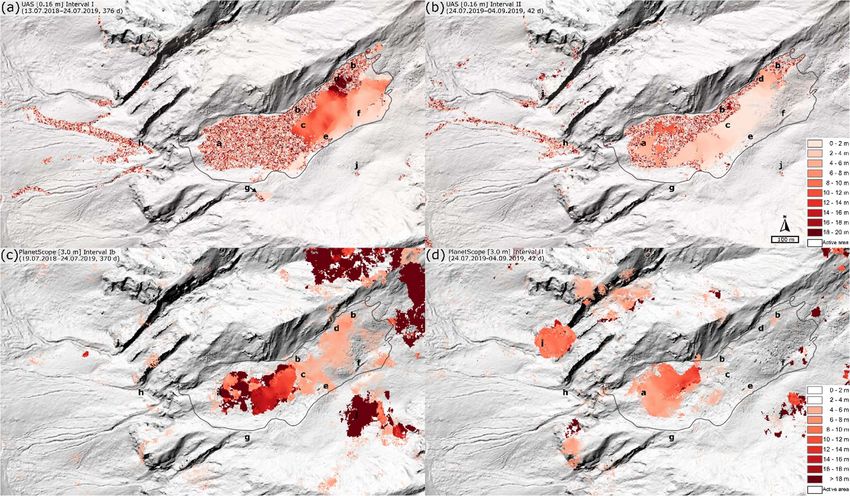
Figure 2 (a) Overview map Austria (Österreichischer Bundesverlag Schulbuch GmbH & Co. KG and Freytag-Berndt & Artaria KG,
Wien). (b) Sattelkar, 30.6.2019 with the debris cone of the 2014 debris flow event and (c) UAS orthophoto (04.09.2019, 1:1.000) showing
boulder sizes of 5–10 m used for manual motion tracking, (d) active boulder blocks from the central AoI.
In August 2014, heavy ongoing precipitation triggered massive debris flow activity of 170 000 m³ in volume, of which
200 approximately 70 000 m³ derived from the catchment above 2 000 m. A further 100 000 m³ was mobilised in the channel
within the cone. The consequence was that the Obersulzbach river was blocked leading to a general flooding situation in the
catchment, resulting in substantial destruction in the middle and lower reaches (Fig. 3).
6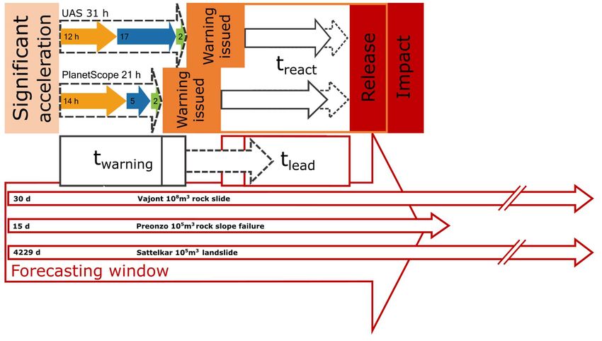
Figure 3 Obersulzbach valley, flood event September 2014. (a) Flooding situation in the Obersulzbach valley with the Sattelkar landslide
205   cone deposit (image centre). (b) Flood area at the valley mouth in Sulzau and Schaffau. The Salzach river is at the bottom of the image.
      ©Salzburger Nachrichten/Anton Kaindl.

      The Sattelkar has been the focus of international research projects such as “PROJECT Sattelkar“ (GeoResearch, 2018) and
      AlpSenseBench (TUM, Chair of Landslide Research, 2020) since 2018. In 2015 preliminary findings revealed a mass
      movement coverage of 130 000 m² with approximately 1 mio. m³ of debris and displacement rates of more than 10 m a-1.
210   The debris consists of boulders up to 10 m in diameter (Fig. 2c, d) allowing visual block tracking and delimiting the active
      process area. High displacement was measured between 2012 and 2015 with up to 30 m a-1.
      In the Sattelkar cirque, several monitoring components are installed to provide ongoing and long–term monitoring. Nine
      permanent ground control points (GCPs) measured with a dGPS to provide stable and optimal conditions to derive
      orthophotos from highly accurate UAS images (GeoResearch, 2018). A total number of 15 near surface temperature loggers
215   (buried at 0.1 m depth) recorded annual mean temperatures slightly above the freezing point (1–2 °C) in the period 2016 to
      2019. Ground thermal conditions at depth react with significant lag times to recent warming and therefore are primarily
      determined by climatic conditions of the past (Noetzli et al., 2019). Significantly cooler climatic conditions in previous
      decades and centuries (Auer et al., 2007) thus likely contributed to the formation of (patchy) permafrost at the Sattelkar
      cirque. Recent empirical–statistical modelling of permafrost distribution in the Hohe Tauern Range confirms possible
220   permafrost presence at the study site (Schrott et al., 2012).

      The Sattelkar is a suitable case study as it is in the early stages of the landslide development and thus fits best to this
      conceptual approach. Here, processes take place on time scales appropriate for long–term observation to provide sufficient
      warning time. The active part of the cirque has accelerated in recent years allowing the analysis of EWS concepts based on
225   multispectral optical remote sensing data supported by complementary block tracking.

      4 Materials and Methods

      4.1. Optical imagery

      Optical satellite imagery is more appropriate for high deformation studies than radar applications due to the high spatial
      resolution as well as the short time span between acquisitions (Delacourt et al., 2007). Although the west–facing slope is
230   favourable for the application of radar derivatives (InSAR/DInSAR), the choice to use optical imagery is based on the
      observed high displacement rates, which cause decorrelation when using radar technologies as they are more sensitive than
      optical technologies. Complex and/or large displacement gradients make the phase ambiguity difficult to solve for radar
      interferometry (Kääb et al., 2017). Revisit times of current radar satellites (e.g. Sentinel–1) are longer than those of optical
      satellites, and if time periods between image acquisition become too long, ground motion may accumulate such that the

                                                                         7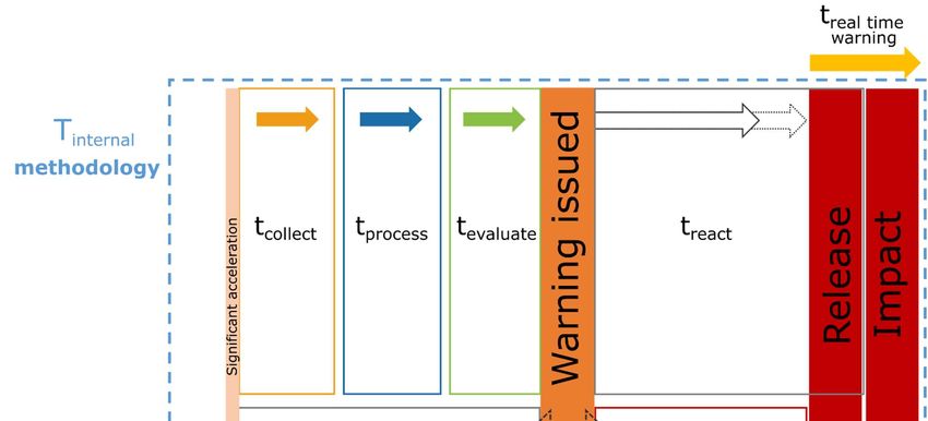
235   displacement is too high to be measured. Several studies on displacements of faults and landslides have shown the potential
      of optical data to provide detailed displacement measurements based on image correlation techniques (DIC) (Leprince et al.,
      2007; Rosu et al., 2015). A further advantage of optical images for geomorphological processes in steep terrain is their
      viewing geometry (close to nadir) (Lacroix et al., 2019). Here we employ DIC to compare the spatiotemporal resolution of
      multispectral optical imagery (UAS and PlanetScope) and to assess its suitability for early warning purposes. UAS images
240   offer excellent spatial resolution and accuracy at the centimetre scale (Turner et al., 2015) and complement large scale
      satellite or airborne acquisitions (Lucieer et al., 2014). PlanetScope imagery provides the highest temporal resolution among
      available sensors with daily acquisitions, guaranteed data availability, and free and open access for research purposes. In this
      study the PlanetScope Analytic Ortho Scene SR (surface reflectance) imagery (16–bit, geometric–, sensor– and radiometric
      corrections) was employed (Planet Labs, 2020b) and was supported by the Planet Labs Education and Research Program.

245   4.2. Data availability of PlanetScope

      Research on the availability and usability of PlanetScope imagery was conducted on the Planet Explorer data hub for the
      time span from the beginning of April to the end of October in 2019, as during these months snow cover should be
      negligible. Filter parameters were solely set for 4–band PlanetScope Ortho Scenes and the Sattelkar AoI. In order to obtain
      all available images, no filters (e.g. sun azimuth, off nadir angle) were applied. We defined four categories i) meteorological
250   constraints due to snow cover, cloud cover and cloud shadow; ii) image (coverage) errors made by the provider, iii) no data
      availability and iv) the remainder of usable data (Table 2). The output request was evaluated according to the defined
      categories and was compared to the provider’s guaranteed daily image provision, which is comprised of 213 days for the
      time period (01.04.2019–31.10.2019). We calculated percentages for the above categories based on days per month as well
      as a seven–month sum and percentage average. The availability analysis did not include an examination of the data with
255   regard to its spatial usability: positional accuracy and/or image shifts.

      Table 2 PlanetScope 4–band data availability and usability for Sattelkar AoI for April to October 2019.

                                                April      May       June        July     August September October 7 month 7 month
      Month
                                                (%)        (%)        (%)        (%)       (%)         (%)        (%)     sum        avg (%)
      usable                                    0.0 %       0.0       20.0       22.6       9.7        13.3       9.7     23          10.7
      unusable
                    cloud cover/shadow             16.7       6.5        0.0       19.4      32.3          16.7     9.7         31      14.5
                    snow cover                     10.0       0.0       33.3        0.0       0.0           3.3     3.2         15       7.0
                    image errors                   23.3      25.8       16.7       12.9      29.0          20.0    19.4         45      21.0
                    no coverage/data voids         10.0      12.9       16.7       32.3      16.1          20.0    32.3         43      20.1
      not available no upload                      40.0      54.8       13.3        9.7      12.9          26.7    25.8         56      26.2

260   Unfavourable meteorological influences of cloud cover/shadow and snow cover affected up to 32.3 % and up to 33.3 %,
      respectively, on all 213 days; on average 14.5 % and 7 % of the days were not usable (Table 2). For 10 days in June snow
      influence had the greatest negative share (33.3 %), for April there were three days of snow coverage and the months
      September and October each had one day of snow coverage. Cloud cover/shadow exerted a higher impact on data usability
      by 14.5 %. Problems on the part of PlanetLabs made much of the data unusable due to image errors; between four and nine
265   images per month were not usable (21 %). On average for 26.2 % of the analysed time period no image data was available.
      In this seven–month period, 43 images (20.1 %) had data voids or did not cover the AoI, thus the overall usability is limited
      to about 11 %.

      4.3. Data Acquisition and Processing

      In line with the concept in Fig. 1 (Sect. 1), the following processing steps are categorised and described.

                                                                             8
270   (1) tcollect: UAS data acquisition was preceded by detailed flight route planning and checks of local weather and snow
      conditions. UAS flights were carried out with a DJI Phantom4 UAS on 13.07.2018, 24.07.2019 and 04.09.2019 (see Table 3,
      Fig. 4, Fig. 6b, c).
      Table 3 Acquisition dates of UAS and PlanetScope images, in chronological order.

      Acquisition set          UAS                           PlanetScope
      (1)                      13.07.2018                    02.07.2018 (a), 19.07.2018 (b)
      (2)                      24.07.2019                    24.07.2019
      (3)                      04.09.2019                    04.09.2019

275   For each acquisition, the total area was covered by four flights which were started on different elevations (Table 4). Flight
      planning was done with UgCS maintaining a high overlap (front: 80 %, side: 70 %) and a target ground sampling distance
      (GSD) of 7 cm. The area covered was approximately 3.4 km² and with a flight speed of about 8 m/s total flight time took
      3.5 hours. The images were captured in RAW format. In the Planet Explorer Data Hub, PlanetScope Ortho Scenes were
      selected for usability; imagery affected by snow cover, cloud cover, cloud shadow and partial AoI coverage was discarded
280   (Table 5).

      Table 4 UAS Flight plans.

      Flight plan       Length of             Flight time Passes   No. of            GSD    Altitude start     Highest flight   Lowest terrain
      parts             flightpath [km]       [min]                images            [cm]   point [m]          position [m]     point [m]
      Top                               6.8            17      6        121             7               2630             3120               2365
      Middle                            7.5            19      6        135             7               2200             2682               1820
      Low 1                             7.3            17      6        130             7               1768             2115               1620
      Low 2                             5.6            14      6            81          7               1768             2110               1620
      Total                            27.2            67     24        467             7                                3120               1620

      Table 5 Planet Scope Ortho Scenes.

      Acquisition       Acquisition       Identifier                                             Incidence Angle
      Date              time (local)                                                             [deg]
         02.07.2018             11:34          20180702_093434_0f3f_3B_AnalyticMS_SR                     2.18E-01
         19.07.2018             11:35          20180719_093512_0f3f_3B_AnalyticMS_SR                     2.36E-01
         24.07.2019             11:42         20190724_094200_1014_3B_AnalyticMS_SR                      5.57E+00
         04.09.2019             11:36         20190904_093632_0e20_3B_AnalyticMS_SR                      4.24E+00
285
      (2) tprocess: In phase two (time to process) the PlanetScope images were visualised in QGIS. Thereafter, a second selection
      (visually with the ‘Map Swipe Tool’ plugin) from the downloaded images was filtered for errors of location, inter–tile shift
      and shifts in the individual bands which were previously not clearly discernible in the online data hub. The final selection of
      images was made based on the temporal proximity to the UAS data to guarantee the best comparability. For acquisition set
290   (1), there are two PlanetScope images (02.07.2018 and 19.07.2018) which differed from the UAS acquisition date
      (13.07.2018) by 11 and 6 days, respectively. For acquisition sets (2) and (3), PlanetScope and UAS acquisition dates were
      identical (24.07.2019 and 04.09.2019). The acquired data sets were categorised in chronological intervals I/Ia/Ib and II (see
      Fig. 4).

                                                                                 9
295   Figure 4 Acquisition dates of UAS and PlanetScope images within the investigated time period. Calculated interval I for UAS images
      (13.07.2018–24.07.2019, 376 d) and interval Ib for PlanetScope images (19.07.2018–24.07.2019, 370 d), interval II for UAS and
      PlanetScope images (24.07.2019–04.09.2019, 42 d). Note: Ia PlanetScope interval was discarded.

      The UAS images in RAW format were modified using Adobe Exposer to improve contrast, highlights, shadows and clarity.
300   Thereafter, they were exported as JPG (compression 95 %) and processed with Pix4Dmapper to 0.08 m resolution and
      orthorectified based on nine permanent ground control points (GCP, 30 x 30 cm). These were repeatedly (1000
      measurements/position) registered with the TRIMBLE R5 dGPS and corrected via the baseline data of the Austrian
      Positioning Service (APOS) provided by the BEV (Bundesamt für Eich– und Vermessungswesen). Horizontal root–mean–
      squared errors (RMSE) range from 0.05 m to 0.10 m for vertical RMSE. These GCPs were employed for georeferencing and
305   further rectification of all UAS surveys.
      Next, the data was clipped to a common area of interest (AoI) and resampled with GDAL and the cubic convolution method
      to 0.16 m to enhance processing time and increased reliability of image correlation. PlanetScope Satellite images were co–
      registered in Matlab relative to a reference image (https://gitlab.lrz.de/tobi.koch/satelliteregistration.git). A feature point
      detection step was applied to estimate a geometric similarity transformation between the reference (master) and all target
310   (slave) image pairs excluding the AoI with its terrain motion. Thereafter feature point outliers were statistically removed
      (RANSAC) and the similarity transformation of the slave images to the master image was performed. After removing the
      outliers, more than 500 feature matches were found for the entire image pair dataset. The mean distance of transformed inlier
      feature points from the target image to their corresponding feature matches in the reference image ranged between 0.6 and
      0.8 pixels, confirming the high registration accuracy (see OSM Fig. 14). We used digital image correlation (DIC) to measure
315   the displacement for the active landslide body of the Sattelkar and to assess the suitability of the PlanetScope and UAS data.
      This method employs optical and elevation data and calculates the distance between an image pair, based on the spatial
      distance of the highest correlation peaks between an initial search and a final reference window. The result provides
      displacement and ground deformation in 2 D on a sub–pixel level. COSI–Corr (Co–registration of Optically Sensed Images
      and Correlation), a widely used software in landslide and earthquake studies was used for sub–pixel image correlation
320   (Stumpf, 2013; Lacroix et al., 2015; Rosu et al., 2015; Bozzano et al., 2018). COSI–Corr is an open source software add–on
      developed by CALTECH (Leprince et al., 2007), for ENVI classic. There are two correlators; in the frequency domain based
      on FFT algorithm (Fast Fourier Transformation) and a statistical one. Applying the more accurate frequential correlator
      engine, recommended for optical images, different parameter combinations of window sizes, direction step sizes and
      robustness iterations were tested. Parameter settings include the initial window size for the estimation of the pixelwise
325   displacement between the images and the final window size for subpixel displacement computation in x, y; a direction step
      in x, y between the sliding windows; and several robustness iterations (Table 6). We utilised recommended window sizes as
      suggested by Leprince et al. (2007) and Bickel et al. (2018). Step size one showed good results while keeping the original
      spatial resolution for the output; robustness iterations of two to four were sufficient for our purposes. Initial and final
      window sizes were systematically tested (see Table 6). For computing a state–of–the–art powerstation was employed (AMD
330   Ryzen 9 3950X 16–core processor, 3.70 GHz, 128 GB RAM).

      Table 6 COSI–Corr input parameters for intervals of UAS and PlanetScope.

      Sensor Resolution     Input interval                         Initial window Final window   Robustness Step size
                                                                   [pix]           [pix]         iteration
      UAS                   I: 13.07.2018–24.07.2019                       128x128         32x32           2      1x1
      [0.16 m]              II: 24.07.2019–04.09.2019
      PlanetScope           Ib: 19.07.2018–24.07.2019                       64x64          32x32             4        1x1
      [3.0 m]               II: 24.07.2019–04.09.2019

                                                                      10
The results of each correlation computation returns a signal–to–noise ratio map (SNR) and displacement fields in east–west
335 and north–south directions. These results were exported from ENVI classic as GTiff and the total displacement was then
calculated with QGIS.
(3) tevaluate: In the last phase (time to evaluate) the results of various parameter settings were compared in QGIS and ArcGIS
along with different combinations of visualisation. Displacement below a 4 m threshold was discarded from the PlanetScope
datasets due to aberrant values (noise, outliers). The threshold definition was defined on (i) the value distribution in both the
340 total displacement and the corresponding SNR result, and (ii) a visual comparison of the maps for the total displacement and
the SNR. This definition allowed us to identify outliers and unlikely displacement. Apart from this threshold no other filters
were employed, and we kept the output raw (see for raw DIC on PlanetScope OSM Fig. 13). Very few inconsistencies were
present in the UAS–derived displacement results, which were accepted without modification.
Additional analyses were performed to estimate the DIC outputs of both, the UAS orthophotos and PlanetScope satellite
345 imagery. Visual tracking of 36 single blocks, identifiable in the UAS orthophoto series allowed deriving direction and
amount of movement; this supported the confirmation process for (i) the total displacement and (ii) the results of automated
and manual tracking. In the next section we present this approach only for time interval II.
5. Results
In Sect. 5.1. we present ground motion results from DIC for the original input resolution for i) UAS, 0.16 m and ii)
350 PlanetScope, 3 m input resolution based on parameters in Table 6. In Sect. 5.2. DIC results for UAS, 0.16 m are analysed
with regard to displacement of visual single block tracking. Finally, in Sect. 5.3. required times for tcollection, tprocessing and
tevaluation for each sensor are presented.
5.1. Total displacements
355 Figure 5 Results of DIC total displacement of orthoimages UAS for (a) and (b) at 0.16 m resolution and PlanetScope (c) and (d) at 3 m
resolution. Time intervals for UAS image pair (a) I (13.07.2018–24.07.2019, 376 d), (b) II (24.07.2019–04.09.2019, 42 d), for
PlanetScope (c) Ib (19.07.2018–24.07.2019, 370 d) and (d) II (24.07.2019–04.09.2019, 42 d).Explanation of inconsistently tracked
features (a), a and b, and (b), b and the northwestern landslide head, are described in 5.2. The solid black line represents the boundary of
the active landslide based on field mapping. Background: hillshade of Lidar DEM, 1 m resolution (© SAGIS).
11360 Figure 5a and Fig. 5b show the total displacements derived from UAS orthophotos at 0.16 m resolution for time intervals I
and II (see Table 6). Apart from several minor displacement patches, no motion is visible outside the active body in either
period. Time interval I (376 d) (Fig. 5a) shows mean displacement values from 6 to 14 m for a coherent area in the eastern
half of the lobe from the centre (c) to the eastern boundary of the active area. The highest displacement rates (up to 20 m) are
observed within small high–velocity clusters in the northwest section (d). Lower velocities occur along the southern
365 boundary (e, f), ranging from zero to 6 m with smooth transitions. Ambiguous, small–scale patterns with highly variable
displacement rates are present in the western half (a) and along the northern boundary (b). No motion is detected along the
western fringe (i.e. at the landslide head) which is 20 m in width. South of the landslide (g) there is a small patch of minor
displacement with continuous (up to 3.5 m) and ambiguous signals. Furthermore, we observed small–scale patterns of
ambiguous signals in the east (j) and in the west of the active area in the drainage channels (h, i).
370 Time interval II (42 d) (Fig. 5b) shows great similarity to time interval I with ambiguous signals in the same areas such as
the drainage channels (h, i) and within the western half of the active area (b). In contrast to interval I (Fig. 5a), within the
active area a homogenous higher velocity patch (up to 6 m) near the landslide head is evident (a). In the eastern half large
homogenous patches extend from the landslide centre (c) to the root zone (d) showing coherent displacement values of zero
to 4 m. During this shorter time interval II, no displacement is detected along the south eastern boundary (e) and for large
375 parts of the root zone (f) previously covered in I. Similar to I, the landslide head has a 20 m rim free of signal (also see Fig. 6
x, y). In the central part of the lobe (c) total displacements are significantly reduced.
Figure 5c and Fig. 5d demonstrate total displacement for similar time intervals to UAS (see Table 3 and Fig. 4). For
interval Ib (370 d) (Fig. 5c) wide fringes with no motion were detected around an actively moving core area, which consists
of small–scale clusters with variable total displacement in the western part, coherent high velocities in the middle, and
380 coherent low velocities east of this core area. Outside the landslide, northeast and immediately south (j), high–velocity
patches are observed.
In interval II (42 d) (Fig. 5d) the detected displacement is restricted to the western half of the landslide (a) and shows the
same significant fringes with no motion as in I. Compared to interval I the motion pattern of this core area is more
homogeneous with increasing displacement towards the east. Outside the active area several patches show medium to high
385 total displacement, the largest of which is located 300 m northwest of the landslide (i).
5.2. Single Block Tracking
Figure 6a illustrates the total displacement derived from the UAS data at high resolution (0.16 m) for interval II (42 d). UAS
orthoimages were used to manually measure single block displacement for 36 clearly identifiable boulders on the landslide
surface. Block displacements of 1 m are visible in the eastern part (f), whereas DIC does not reveal any displacement below
390 1 m. Boulder tracks longer than 2 m in the central and western part of the landslide are reflected by DIC–derived
displacement values. Near the front a 6 m displacement of one block (a) is represented in the DIC result. The highest values
(6 m, 10 m, 16 m) were observed in regions where DIC delivered ambiguous, small–scale patterns of highly variable
displacements. Displacement vectors show consistent bearings in the downslope direction of the landslide motion for
homogeneous areas of the DIC result (a, c, d); there are short vectors with chaotic bearings in areas of ambiguous patterns
395 (b), some of which are pointing upslope. The vectors show no displacement in stable areas outside the active area and where
no DIC signal is returned.
12Figure 6 (a) Displacement derived from UAS data at 0.16 m resolution for interval II (24.07.2019–04.09.2019, 42 d) combined with
boulder trajectories (in metres) manually measured in the UAS orthophotos in the same time period. Displacement vectors showing
400 landslide flow (black). Origin of inconsistently tracked features (a) for b and the northwestern landslide head are described in 5.2. The
solid black line represents the boundary of the active landslide based on field mapping. Background: UAS hillshade, 24.07.2019 (0.08 m),
orientation -3° from north. UAS orthophotos at 0.16 m resolution for the master (b) and slave image (c) of the corresponding time interval.
5.3. Time required for collection, processing and evaluation
405 In Sect. 2 we introduced a novel concept to extend lead time, consisting of three phases within the warning time window (see
Fig. 1). This concept is based on DIC results, thus every step comprised in each phase has been previously undertaken. On
this basis, knowledge of required time for a further process iteration of the three phases is given.
Time required for collection, processing and evaluation of UAS and PlanetScope data are estimated and summed in Fig. 7.
PlanetLabs specifies 12 hours from image acquisition to the provision in the data hub, which includes to a large amount data
410 pre–processing (Planet Labs, 2020b). Adding two hours for the selection, order and download process, we assume that time
required for the collection phase is approximately the same for both sensors, with 14 hours for PlanetScope and 12 hours for
13UAS. With regard to the time needed for the processing phase, the sensors differ with UAS requiring 17 hours and
PlanetScope five hours. Time for the evaluation phase is estimated to be about two hours. In sum, twarning for UAS is
approximately 31 hours compared to 21 hours for PlanetScope.
415
Figure 7 Time to warning is composed of three phases: time to collect, to process and to deliver. Time to warning (subsequent to
acceleration) is 21 h for PlanetScope and 31 h for UAS. Thus, any hazard process that takes longer than 21/31 h to prepare the release and
impact can be forecasted.
6 Discussion
420 To systematically analyse the predictive power of the UAS and PlanetScope data, we will (i) evaluate ambiguous signals,
error sources and output performance, (ii) assess obtainable temporal and spatial resolution and (iii) derive a systemic
estimate of the minimum obtainable warning times.
6.1. Error sources and output performance
To evaluate error sources and output performance, we compared results of digital image correlation results from optical data
425 with (i) high resolution UAS orthophotos, (ii) mapped mass movement boundary and (iii) visual block tracking for UAS
orthophotos. The approximately one year evaluation period encompassed all seasons, hence freezing/thawing conditions and
a wide range of meteorological influences, e.g. thunderstorms and heavy rainfall, are included. The two investigated time
intervals are I/Ib and II, covering 376/370 days and 42 days (typical high–alpine summer season), respectively (Fig. 4).
Interval II exclusively covers (high–alpine) summer conditions, with negligible to no contribution from freezing conditions.
430 As these inclusion periods are inconsistent, the amount of total displacement cannot be directly compared; however the
relative motion patterns can be. Accordingly, we can confirm the suggested parameter settings of earlier studies on window
sizes, steps and robustness iterations (Ayoub et al., 2009; Bickel et al., 2018).
In terms of the mass movement boundary, the total displacement derived from the DIC of the UAS data generally matches
the field–mapped landslide boundary for both intervals (I, II) (Fig. 5a, b), and is supported by the absence of significant
435 noise outside the AoI. Mapped boulder trajectories for interval II (see Fig. 6) are consistent with the calculated total
displacement and thus confirm COSI–Corr as a reliable DIC tool to derive ground motion for this study site and UAS
orthophotos as suitable input data. Nevertheless, there are several areas with ambiguous signals. Here we follow Leprince et
14al. (2007) describing a correlation loss as ‘decorrelation’ with signal–to–noise values of low/null (i.e. no convergence of the
correlation algorithm) and/or large offsets, either unrealistic in nature or beyond the valid matching window distance.
440 Decorrelation in our understanding exhibits a salt–and–pepper appearance in the DIC result with random displacement
vectors, related to inconsistently tracked features. The software is not able to find the corresponding, correlated surface
pattern, leading to a misfit (i.e. misrepresentation) and/or mismatch (i.e. blunders) of the matching windows and finally
resulting in noise (Debella-Gilo, 2011; Guerriero et al., 2020). Nevertheless, this decorrelation signal is still a valuable
observation that might be related to surface processes and not only to erroneous limitations of the DIC method. There are
445 three main reasons that might cause these effects: (i) significant temporal change of the surface, i.e. revolving and/or
rotational deformation, (ii) high displacements exceeding the matching window size being smaller than the offset, (iii) land
cover changes such snow cover, vegetation cover and alluvial processes, among others, and (iv) changes related to
illumination (e.g. shadow) or image errors (e.g. orthorectification, shifts in individual bands) (Leprince, 2008; Debella-Gilo,
2011; Lucieer et al., 2014; Stumpf et al., 2016). In our study, the decorrelated salt–and–pepper areas include to a large
450 degree the landslide head (a), the drainage channel (h) (Fig. 5a, b), a larger patch south of the active area boundary (g)
(Fig. 5a), and some smaller ones in little depressions (g) (Fig. 5a) and (j) (Fig. 5a, b). The patches (j) and east of (j) are
identified as snow fields in the orthophotos and the noise results from decorrelation. In Fig. 5a, the large southern patch (g)
shows clear displacement values for the rear part and decorrelation for the front region resulting from morphological changes
within the image pair of interval I (see OSM Fig. 12). This is due to a gain between 1 and 2 m for an area of about 250 m².
455 The decorrelation in the drainage channel (h) could stem from massive changes in pixel values, similar to the decorrelation
on the basis of alluvial processes, as described by Leprince et al. (2007). Decorrelations in the areas with the fastest ground
motions also lead to high pixel changes (Stumpf et al., 2016): these are observable in the active landslide area within the
lobe, where large areas of decorrelation may be explained by high displacements in the leading landslide head (a) with
redetected, hence correlated pixels in the trailing areas (c, d, e, f). These findings can be transferred to the landslide interior
460 area (a, b), the frontal western regions and the northern margin (b). The observation is confirmed by geomorphological
mapping (see OSM Fig. 11) and measured boulder block trajectories from the orthophotos (Fig. 6a). Several patches of
correlation (c, f) with corresponding boulder trajectories up to 4 m (34.8 m yr-1) (d) can be detected in the rear areas. A
correlated patch with a 16 m (34.8 m yr-1) trajectory (a) is located in the flow direction behind the foremost boulder. In this
case the method was able to partially capture the displacement as the distinct boulder block supported the detection, which
465 probably led to correlation. Similarly there is another example with a trajectory of 10 m (86.9 m yr-1) outside a homogeneous
correlated area. This leads to the assumption that for the calculated time period, with 63 pixels or more at a resolution of 0.16
m, no pixel matching is possible and probably reached the correlation capacity due to the too high displacement. With a
correlation window smaller than the displacement, the algorithm cannot capture the displacement (Stumpf et al., 2016).
However as field observations provide evidence that the rock masses are deforming, and the surface is altering due to the
470 high mobility and rotational behaviour of some boulder blocks. This leads to changed pixel values and spectral
characteristics of the block surface and the surrounding area, which can also result in poor correlations, and even random
errors and mismatches (Debella-Gilo and Kääb, 2011). This finding is similar to observations in a rock glacier study by
Debella-Gilo and Kääb (2011). Similar results were observed by Lucieer et al. (2014), who described a loss of recognisable
surface patterns if revolving and rotational displacements occur, causing decorrelation and a noise as output. These results
475 show that with COSI–Corr and UAS orthophotos of 0.16 m, it is possible to detect the total displacement of the landslide in
both extent and internal process behaviour even in this steep, heterogeneous terrain. Nevertheless, high displacement rates
and rotational surface behaviour in the cirque limit the DIC method. A decrease of the time interval for this particular highly
mobile study site would likely reveal an enhanced correlation since for shorter time periods the total displacement decreases,
and surface changes are reduced, which can be controlled by shortening the temporal baseline (Debella-Gilo and Kääb,
15480 2011). In sum, though the results contain heterogeneous, noisy, decorrelated areas, the combination with homogeneous
displacement areas still offers valuable insights into this and other internal landslide structures and complex behaviours.
6.2. Comparison of temporal and spatial resolution
We compared the COSI–Corr total displacement results of PlanetScope (Ib and II, Fig. 5c, d) and UAS images (I and II,
Fig. 5a, b and Fig. 6a) for the same time periods at different spatial resolutions (see Table 6). For the PlanetScope DIC result
485 the main part of the landslide is detected, and its area is generally consistent with the results of the UAS DIC, which is
additionally confirmed by boulder trajectories. The frontal part (a) reveals correlation signals (I and II); while for the same
time intervals and parts, the UAS DIC results show a decorrelation (Ib and II). The correlation is likely to be attributable to
the coarser spatial resolution of 3 m PlanetScope input data, hence a smaller number of pixels to be captured at this site with
the DIC method. Similar texture of rock clast surfaces could lead to false positives resulting in correlation as patches appear
490 similar in matching windows. However, in contrast to the UAS result (Fig. 5a, b), the outcome on a large scale fails to detect
the entire actual active area (b), (f) as well as its internal motion behaviour. Nevertheless, for the visualisation and analysis of
the PlanetScope results, the range of total displacements had to be restricted to values equal to and greater than 4 m due to
noise and outliers over large areas, as applied and described by Bontemps et al. (2018). Even then, noise and several
misrepresented displacement patches are observed for (i, j) and in the northeast image corner (Fig. 5). We can identify
495 several reasons for these large clusters of high motion values. Massive cloud and snow coverage hampered both first images
of interval Ib (19.07.2018) (Fig. 5c) and II (24.07.2019) (Fig. 5d), leading to a 20 m fringe of false displacements in the
north–eastern part of the image. Minor snow fields as visible in the images from 24.07.2019 for both, the UAS and
PlanetScope, likely explain the big cluster of incorrect displacement southeast of the lobe (j); nonetheless, in the satellite
image they are smaller than the resulting DIC displacement. High cloud coverage in two input images with large areas of
500 white pixels may exert an influence leading to high gains due to sensor saturation (Leprince, 2008). Illumination changes in
interval II (Fig. 5d) may cause unrealistic displacements outside the boundary with slightly darker colours due to shadows in
the first satellite image (24.07.2019) and large parts within the second image (04.09.2019) are also in the shade. A
comparison of the acquisition times and true sun zenith, e.g. for the second image, reveals a difference of 01:34 h between
the image acquisition at 11:36 LT (local time) and the true local solar time at 13:10 LT. As the study site is located in a
505 high–alpine terrain with a west facing cirque, at this time of day there are shadows of considerable length which have a
significant influence on the result of digital image correlations. One clear advantage of the UAS images is that their
acquisition is plannable according to the best illumination conditions with the sun at its zenith. Moreover, the UAS flight
path as well as the system itself remained the same for all three acquisitions, while PlanetScope employs various satellites.
Despite different input resolutions and time intervals (Ib vs. I and II vs. II, see Table 3) with different sensors (UAS,
510 PlanetScope) there is a similarity for the landslide head which indicates that the displacement is restricted to a smaller area
than the previously demarcated boundary, based on our field investigations. This is clearer for the time interval I (376/370 d)
(Fig. 5a vs. c) as for the longer temporal baseline the total displacement accumulation is higher, thus better captured by
COSI–Corr for PlanetScope 3 m resolution. Due to the shorter interval II (42 d) (Fig. 5b vs. d) with less accumulated total
displacement, the rear of the landslide is not represented; no signal is shown as the total displacement for PlanetScope was
515 restricted to values above 4 m. Values below 4 m had to be discarded for PlanetScope DIC results as they were lost in noise,
i.e. for the entire DIC results there is total displacement between 0 m and 4 m (cf. the online supplementary material (OSM)
Fig. 13). Hence, when applying a minimum threshold of 4 m, the satellite image detects large parts of the main active core
area but widths of 50–80 m from the boundary show no displacement. However, false large clusters of high total
displacement are within the PlanetScope result interval I for (j) and the northeast image corner (Fig. 5c), and interval II for
520 (i) (Fig. 5d).
16You can also read