Interpretable serious event forecasting using machine learning and SHAP - Sebastian Gustafsson
←
→
Page content transcription
If your browser does not render page correctly, please read the page content below
Examensarbete 30 hp
                                             6 juni 2021

Interpretable serious event
forecasting using machine learning
and SHAP

Sebastian Gustafsson

          Civilingenjörsprogrammet i informationsteknologi
           Computer and Information Engineering Programme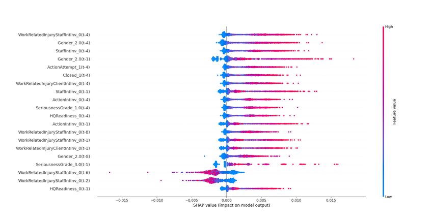
Abstract

Institutionen för
                                    Interpretable serious event forecasting using
informationsteknologi               machine learning and SHAP
Besöksadress:
ITC, Polacksbacken                  Sebastian Gustafsson
Lägerhyddsvägen 2

Postadress:                         Accurate forecasts are vital in multiple areas of economic, scientific, commercial, and
Box 337                             industrial activity. There are few previous studies on using forecasting methods for pre-
751 05 Uppsala                      dicting serious events. This thesis set out to investigate two things, firstly whether ma-
                                    chine learning models could be applied to the objective of forecasting serious events.
Hemsida:
                                    Secondly, if the models could be made interpretable. Given these objectives, the ap-
http:/www.it.uu.se
                                    proach was to formulate two forecasting tasks for the models and then use the Python
                                    framework SHAP to make them interpretable. The first task was to predict if a serious
                                    event will happen in the coming eight hours. The second task was to forecast how many
                                    serious events that will happen in the coming six hours. GBDT and LSTM models were
                                    implemented, evaluated, and compared on both tasks. Given the problem complexity of
                                    forecasting, the results match those of previous related research. On the classification
                                    task, the best performing model achieved an accuracy of 71.6%, and on the regression
                                    task, it missed by less than 1 on average.

               Extern handledare: Carl Barck-Holst
               Ämnesgranskare: Salman Toor
               Examinator: Lars-Åke Nordén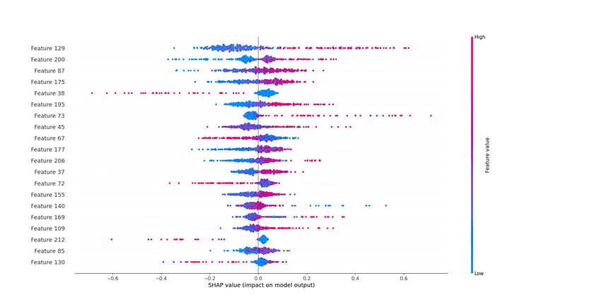
Sammanfattning

Exakta prognoser är viktiga inom flera områden av ekonomisk, vetenskaplig, kommersiell och industri-
ell verksamhet. Det finns få tidigare studier där man använt prognosmetoder för att förutsäga allvarliga
händelser. Denna avhandling syftar till att undersöka två saker, för det första om maskininlärningsmodeller
kan användas för att förutse allvarliga händelser. För det andra, om modellerna kunde göras tolkba-
ra. Med tanke på dessa mål var metoden att formulera två prognosuppgifter för modellerna och sedan
använda Python-ramverket SHAP för att göra dem tolkbara. Den första uppgiften var att förutsäga om
en allvarlig händelse kommer att ske under de kommande åtta timmarna. Den andra uppgiften var att
förutse hur många allvarliga händelser som kommer att hända under de kommande sex timmarna. GBDT-
och LSTM-modeller implementerades, utvärderades och jämfördes för båda uppgifterna. Med tanke på
problemkomplexiteten i att förutspå framtiden matchar resultaten, de från tidigare relaterad forskning.
På klassificeringsuppgiften uppnådde den bäst presterande modellen en träffsäkerhet på 71, 6%, och på
regressionsuppgiften missade den i genomsnitt med mindre än 1 i antal förutspådda allvarliga händelser.

                                                       ii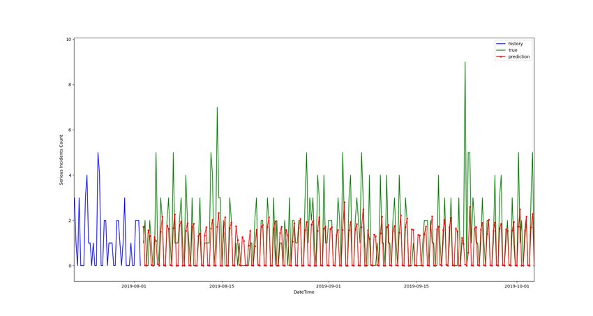
“Don’t ever prophesy; for if you prophesy wrong, nobody will forget it; and if you prophesy right, nobody will
remember it.”
                                                                                                     — Josh Billings

Acknowledgment
I want to thank my supervisor Carl Barck-Holst and Daniel Bernhed at West code solutions for their
encouraging support and assistance during this thesis, and for allowing me to pursue my master thesis
together with them. I want to thank Norah Navér for proofreading and helping me with the report. I
also want to thank my reviewer Salman Toor for his guidance and expertise that helped me during this
project.

                                                        iii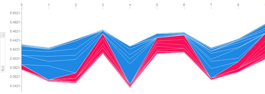
Contents
1   Introduction                                                                                                                                     1
    1.1 Motivation . . . . . . . . . . . . . . . . . . . . . . . . . . . . . . . . . . . . . . . . . .                                               2
    1.2 Objective and Research Question . . . . . . . . . . . . . . . . . . . . . . . . . . . . . .                                                  3
    1.3 Delimitation . . . . . . . . . . . . . . . . . . . . . . . . . . . . . . . . . . . . . . . . .                                               3

2   Related Work                                                                                                                                      4

3   Background                                                                                                                                        6
    3.1 Machine Learning . . . . . . . . . . . . . . . . . . . . .               .   .   .   .   .   .   .   .   .   .   .   .   .   .   .   .   .    6
    3.2 Artificial Neural Networks . . . . . . . . . . . . . . . .               .   .   .   .   .   .   .   .   .   .   .   .   .   .   .   .   .    6
    3.3 Recurrent Neural Networks . . . . . . . . . . . . . . . .                .   .   .   .   .   .   .   .   .   .   .   .   .   .   .   .   .    8
        3.3.1 Standard RNN . . . . . . . . . . . . . . . . . .                   .   .   .   .   .   .   .   .   .   .   .   .   .   .   .   .   .    8
        3.3.2 Long Short-Term Memory . . . . . . . . . . . .                     .   .   .   .   .   .   .   .   .   .   .   .   .   .   .   .   .   12
        3.3.3 Gated Recurrent Unit . . . . . . . . . . . . . . .                 .   .   .   .   .   .   .   .   .   .   .   .   .   .   .   .   .   13
    3.4 Gradient Boosting Decision Trees . . . . . . . . . . . .                 .   .   .   .   .   .   .   .   .   .   .   .   .   .   .   .   .   14
        3.4.1 Decision Trees . . . . . . . . . . . . . . . . . .                 .   .   .   .   .   .   .   .   .   .   .   .   .   .   .   .   .   14
        3.4.2 Gradient Boosting . . . . . . . . . . . . . . . .                  .   .   .   .   .   .   .   .   .   .   .   .   .   .   .   .   .   15
    3.5 Explainable Machine Learning . . . . . . . . . . . . . .                 .   .   .   .   .   .   .   .   .   .   .   .   .   .   .   .   .   17
        3.5.1 Local Interpretable Model-Agnostic Explanations                    .   .   .   .   .   .   .   .   .   .   .   .   .   .   .   .   .   17
        3.5.2 Shapley Additive Explanation . . . . . . . . . .                   .   .   .   .   .   .   .   .   .   .   .   .   .   .   .   .   .   18
    3.6 Data Processing . . . . . . . . . . . . . . . . . . . . . .              .   .   .   .   .   .   .   .   .   .   .   .   .   .   .   .   .   20
        3.6.1 Sliding Window method . . . . . . . . . . . . .                    .   .   .   .   .   .   .   .   .   .   .   .   .   .   .   .   .   20
        3.6.2 Categorical data . . . . . . . . . . . . . . . . .                 .   .   .   .   .   .   .   .   .   .   .   .   .   .   .   .   .   21
        3.6.3 One Hot encoding . . . . . . . . . . . . . . . .                   .   .   .   .   .   .   .   .   .   .   .   .   .   .   .   .   .   21
        3.6.4 Count Encoding . . . . . . . . . . . . . . . . .                   .   .   .   .   .   .   .   .   .   .   .   .   .   .   .   .   .   21

4   Method                                                                                                                                           23
    4.1 System Overview . . . . . . . . . . . . . . . .      .   .   .   .   .   .   .   .   .   .   .   .   .   .   .   .   .   .   .   .   .   .   23
    4.2 Preparing the data . . . . . . . . . . . . . . . .   .   .   .   .   .   .   .   .   .   .   .   .   .   .   .   .   .   .   .   .   .   .   23
    4.3 Hyperparameter Tuning . . . . . . . . . . . . .      .   .   .   .   .   .   .   .   .   .   .   .   .   .   .   .   .   .   .   .   .   .   26
        4.3.1 Tuning the models . . . . . . . . . . .        .   .   .   .   .   .   .   .   .   .   .   .   .   .   .   .   .   .   .   .   .   .   27
    4.4 LSTM models . . . . . . . . . . . . . . . . . .      .   .   .   .   .   .   .   .   .   .   .   .   .   .   .   .   .   .   .   .   .   .   28
        4.4.1 Dense Layer . . . . . . . . . . . . . .        .   .   .   .   .   .   .   .   .   .   .   .   .   .   .   .   .   .   .   .   .   .   28
        4.4.2 Dropout layer . . . . . . . . . . . . . .      .   .   .   .   .   .   .   .   .   .   .   .   .   .   .   .   .   .   .   .   .   .   29
        4.4.3 Regression . . . . . . . . . . . . . . .       .   .   .   .   .   .   .   .   .   .   .   .   .   .   .   .   .   .   .   .   .   .   29
        4.4.4 Classification . . . . . . . . . . . . . .     .   .   .   .   .   .   .   .   .   .   .   .   .   .   .   .   .   .   .   .   .   .   30
    4.5 GBDT models . . . . . . . . . . . . . . . . . .      .   .   .   .   .   .   .   .   .   .   .   .   .   .   .   .   .   .   .   .   .   .   30
        4.5.1 Regression . . . . . . . . . . . . . . .       .   .   .   .   .   .   .   .   .   .   .   .   .   .   .   .   .   .   .   .   .   .   31
        4.5.2 Classification . . . . . . . . . . . . . .     .   .   .   .   .   .   .   .   .   .   .   .   .   .   .   .   .   .   .   .   .   .   32
    4.6 Implementing Explainability . . . . . . . . . .      .   .   .   .   .   .   .   .   .   .   .   .   .   .   .   .   .   .   .   .   .   .   32
        4.6.1 Force plots . . . . . . . . . . . . . . .      .   .   .   .   .   .   .   .   .   .   .   .   .   .   .   .   .   .   .   .   .   .   32
        4.6.2 DeepExplainer . . . . . . . . . . . . .        .   .   .   .   .   .   .   .   .   .   .   .   .   .   .   .   .   .   .   .   .   .   33
        4.6.3 TreeExplainer . . . . . . . . . . . . . .      .   .   .   .   .   .   .   .   .   .   .   .   .   .   .   .   .   .   .   .   .   .   33
        4.6.4 Global . . . . . . . . . . . . . . . . . .     .   .   .   .   .   .   .   .   .   .   .   .   .   .   .   .   .   .   .   .   .   .   34
    4.7 Evaluation Method . . . . . . . . . . . . . . .      .   .   .   .   .   .   .   .   .   .   .   .   .   .   .   .   .   .   .   .   .   .   34
        4.7.1 Receiver operating characteristic curves       .   .   .   .   .   .   .   .   .   .   .   .   .   .   .   .   .   .   .   .   .   .   34
        4.7.2 Geometric Mean . . . . . . . . . . . .         .   .   .   .   .   .   .   .   .   .   .   .   .   .   .   .   .   .   .   .   .   .   35
        4.7.3 Mean Absolute Error . . . . . . . . . .        .   .   .   .   .   .   .   .   .   .   .   .   .   .   .   .   .   .   .   .   .   .   36

                                                     iv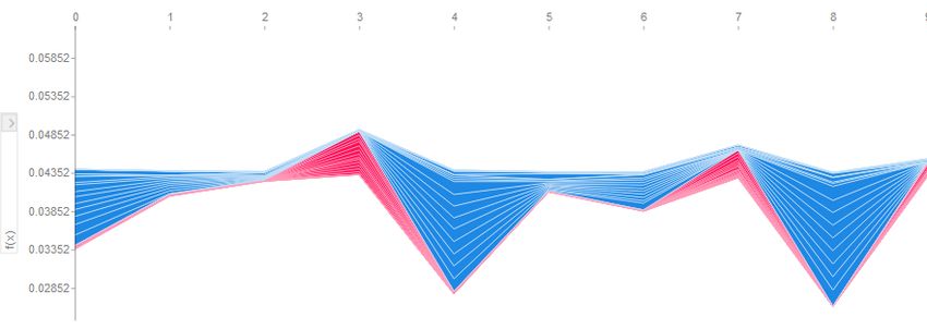
4.7.4    Root Mean Squared Error . . . . . . . . . . . . . . . . . . . . . . . . . . . . .                                                                      36

5   Result                                                                                                                                                               37
    5.1 Model Evaluation . . . . . .     .   .   .   .   .   .   .   .   .   .   .   .   .   .   .   .   .   .   .   .   .   .   .   .   .   .   .   .   .   .   .   .   37
         5.1.1 Regression . . . . .      .   .   .   .   .   .   .   .   .   .   .   .   .   .   .   .   .   .   .   .   .   .   .   .   .   .   .   .   .   .   .   .   37
         5.1.2 Classification . . . .    .   .   .   .   .   .   .   .   .   .   .   .   .   .   .   .   .   .   .   .   .   .   .   .   .   .   .   .   .   .   .   .   39
    5.2 Explanations . . . . . . . .     .   .   .   .   .   .   .   .   .   .   .   .   .   .   .   .   .   .   .   .   .   .   .   .   .   .   .   .   .   .   .   .   41
         5.2.1 GBDT . . . . . . . .      .   .   .   .   .   .   .   .   .   .   .   .   .   .   .   .   .   .   .   .   .   .   .   .   .   .   .   .   .   .   .   .   41
         5.2.2 LSTM . . . . . . . .      .   .   .   .   .   .   .   .   .   .   .   .   .   .   .   .   .   .   .   .   .   .   .   .   .   .   .   .   .   .   .   .   43
         5.2.3 Global explanations       .   .   .   .   .   .   .   .   .   .   .   .   .   .   .   .   .   .   .   .   .   .   .   .   .   .   .   .   .   .   .   .   47

6   Discussion                                                                                                                                                           49
    6.1 Classification task . . . . . . . . . . . . . . . . . . . . . . . . . . . . . . . . . . . . . .                                                                  49
    6.2 Regression task . . . . . . . . . . . . . . . . . . . . . . . . . . . . . . . . . . . . . . .                                                                    50
    6.3 Conclusion . . . . . . . . . . . . . . . . . . . . . . . . . . . . . . . . . . . . . . . . .                                                                     50

7   Future Work                                                                                                                                                          52

                                                                 v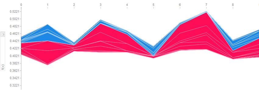
List of Figures
1 An artificial neuron with several inputs and one output. . . . . . . . . . . . . . . . . . . 7
2 A multilayered artificial neural network consisting of three layers. . . . . . . . . . . . . 8
3 The difference between a neuron in an artificial neural network and a neuron in a recurrent
neural network. The difference being the recurring edge. . . . . . . . . . . . . . . . . . 9
4 A neuron in a single-layer recurrent neural network unfolded. On the left is the single-
layer recurrent network folded and on the right unfolded. . . . . . . . . . . . . . . . . . 9
5 A neuron in a multi-layer recurrent neural network unfolded. On the left is the multi-layer
recurrent network folded and on the right unfolded. . . . . . . . . . . . . . . . . . . . . 10
6 An illustration of different sequence modelling types[6]. . . . . . . . . . . . . . . . . . 10
7 An illustration of the problems with long range learning gradients exploding or vanishing. 12
8 An illustration of a long short-term memory cell and its different gates[11]. . . . . . . . 13
9 An illustration of a gated recurrent unit for three time steps[10]. . . . . . . . . . . . . . 13
10 Illustration showing an example of a decision tree. . . . . . . . . . . . . . . . . . . . . . 14
11 An illustration describing the gradient boosting decision trees algorithm on a high level[32].
For each iteration a new decision tree is added, that aims to rectify the errors of previous
trees. . . . . . . . . . . . . . . . . . . . . . . . . . . . . . . . . . . . . . . . . . . . . . 16
12 An illustration showing all different coalitions of three example features in a tree structure. 19
13 An illustration of the implementation process on a high level. . . . . . . . . . . . . . . . 23
14 A high-level overview of the pre-processing steps taken. After the initial three steps the
pre-processing splits into regression, and classification specific pathways. . . . . . . . . 25
15 An illustration of the difference between grid search, on the left, and random search[20]. 27
16 An illustration of a standard neural network and one with dropout applied[25]. . . . . . . 29
17 The layers used in the LSTM regression model. . . . . . . . . . . . . . . . . . . . . . . 30
18 The layers used in the LSTM classification model. . . . . . . . . . . . . . . . . . . . . . 30
19 A flowchart of the walk forward validation algorithm used for regression with GBDT. . . 31
20 An illustration of a force plot, a tool used for explaining predictions provided by SHAP. . 33
21 An illustration of a force plot with three dimensional data where the horizontal axis de-
picts time steps. . . . . . . . . . . . . . . . . . . . . . . . . . . . . . . . . . . . . . . . 33
22 An illustration of a global force summary plot that show the influence of features on a
model in general. . . . . . . . . . . . . . . . . . . . . . . . . . . . . . . . . . . . . . . 34
23 An illustration showing two receiver operating characteristic curves. . . . . . . . . . . . 36
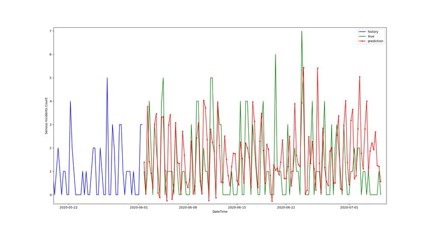
24 Line chart illustrating the performance of the GBDT model on the regression task. . . . . 38
25 Line chart illustrating the performance of the LSTM model on the regression task. . . . . 38
26 A confusion matrix showing the results from the LSTM model on the classification task. 40
27 A confusion matrix showing the results from the GBDT model on the classification task. 40
28 Force plot explaining influential features for the GBDT model on the regression task when
predicting a high value. . . . . . . . . . . . . . . . . . . . . . . . . . . . . . . . . . . . 41
29 Force plot explaining influential features for the GBDT model on the regression task when
predicting a low value. . . . . . . . . . . . . . . . . . . . . . . . . . . . . . . . . . . . 42
30 Force plot explaining influential features for the GBDT model on the classification task
when predicting the false class correctly. . . . . . . . . . . . . . . . . . . . . . . . . . . 42
31 Force plot explaining influential features for the GBDT model on the classification task
when predicting the true class correctly. . . . . . . . . . . . . . . . . . . . . . . . . . . 43
32 Force plot explaining influential features of the LSTM model on the regression task when
predicting a high value, with all time steps. . . . . . . . . . . . . . . . . . . . . . . . . 43
33 Force plot explaining influential features of the LSTM model on the regression task when
predicting a high value, for one time step. . . . . . . . . . . . . . . . . . . . . . . . . . 44
vi
34 Force plot explaining influential features of the LSTM model on the regression task when
predicting a low value, for all time steps. . . . . . . . . . . . . . . . . . . . . . . . . . . 44
35 Force plot explaining influential features of the LSTM model on the regression task when
predicting a low value, the last time step. . . . . . . . . . . . . . . . . . . . . . . . . . . 45
36 Force plot explaining influential features of the LSTM model on the classification task
when predicting a false class, with all time steps. . . . . . . . . . . . . . . . . . . . . . 45
37 Force plot explaining influential features of the LSTM model on the classification task
when predicting a false class, the last time step. . . . . . . . . . . . . . . . . . . . . . . 46
38 Force plot explaining influential features of the LSTM model on the classification task
when predicting a true class, for all time steps. . . . . . . . . . . . . . . . . . . . . . . . 46
39 Force plot explaining influential features of the LSTM model on the classification task
when predicting a true class, the last time step. . . . . . . . . . . . . . . . . . . . . . . . 47
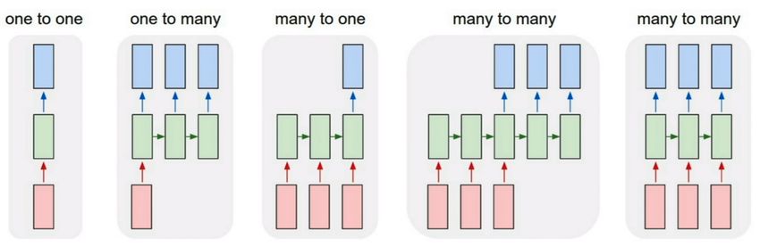
40 Summary plot showing the globally influential features of the GBDT model on the clas-
sification task. . . . . . . . . . . . . . . . . . . . . . . . . . . . . . . . . . . . . . . . . 48
41 Summary plot showing the globally influential features of the LSTM model on the re-
gression task. . . . . . . . . . . . . . . . . . . . . . . . . . . . . . . . . . . . . . . . . 48
viiList of Tables
1 A table of example temperature data. . . . . . . . . . . . . . . . . . . . . . . . . . . . . 20
2 Table of example temperature data after applying the sliding window method. . . . . . . 21
3 Example table of both numerical and categorical data. . . . . . . . . . . . . . . . . . . . 21
4 Table with one hot encoded categorical example data. . . . . . . . . . . . . . . . . . . . 21
5 Table with count encoded categorical example data. . . . . . . . . . . . . . . . . . . . . 22
6 Table showing an example of the pre-processed data for regression. . . . . . . . . . . . . 26
7 Table showing an example of the pre-processed data for classification. . . . . . . . . . . 26
8 Table showing evaluation metrics for both regression models. . . . . . . . . . . . . . . . 37
9 Table showing the evaluation metrics for both classification models. . . . . . . . . . . . 39
viii1 Introduction
1 Introduction
Accurate forecasts are vital in multiple areas of economic, scientific, commercial, and industrial activity.
Examples include sales for a specific product the coming week, electricity consumption during the coming
month, and the coming day’s temperature at a specific location. Knowing the future sales of a product
can help in production planning, knowing electricity consumption can help in directing more power to the
places where the strain will be higher, and knowing the temperature can help an indoor climate system
maintain a good indoor climate. The use cases of having accurate forecasts are evident and one area
where models, statistical, or machine learning are applied on these types of tasks is called time series
forecasting, where predictions are made using data comprised of one or more time series[8].
The type of data required to do time series forecasting is time series data, a set of observations that are
made sequentially through time and can be continuous or discrete. The essential characteristic of time
series data is that there exists a time linked with each observation and that it is ordered by this[8]. With
access to time series data it can be possible to predict the future, and for that, there are multiple different
methods. Practitioners in the area of time series forecasting have historically used linear statistical mod-
els such as Autoregressive Integrated Moving Average(ARIMA)[8]. Still, machine learning models have
established themselves as serious contenders to these classical statistical methods[3].
In 2018, professor Spyros Makridakis organized a competition called M4. The purpose of the competition
was to identify the most accurate forecasting methods for different types of tasks. Three previous versions
of this competition have been held, and for each iteration, the time series data are extended and additional
forecasting methods are introduced, as well as new ways of evaluating the performance of these methods.
The platform Kaggle[1], which is an online community of data scientists and machine learning practi-
tioners, has hosted similar competitions. Article[4] summarizes and showcases what forecasting methods
performed best for six different time series forecasting competitions on Kaggle. The result shows that
four of the competitions were won by non-traditional forecasting methods, namely, two machine learning
approaches called neural networks and gradient boosting decision trees. These competitions drive the
time series forecasting area forward and, give thorough documentation of the performance of different
methods on different types of tasks.
Instead of using the classical approach of statistical models for time series forecasting, it has been shown
that machine learning is a great alternative. As for statistical models, the objective of machine learning
is to discover knowledge from data to make intelligent decisions and, there are a variety of different
types of models and algorithms[21]. Machine learning models, sometimes also called black-box models,
are examples of non-parametric nonlinear models that use only historical data to learn the stochastic
dependency between the past and the future[5]. One sub-domain of machine learning called supervised
learning is comprised by algorithms and models that are well suited for time series forecasting. The
term supervised refers to a set of training samples, also called input signals, where the desired output
signals are already known, also called labels, which means that the correct answer is known. Time
series forecasting tasks can rather straightforwardly be re-framed as supervised learning problems, this
re-framing gives access to a suite of different supervised learning algorithms that can be used to tackle
the problem.
Some machine learning approaches that have been successful at time series forecasting are neural net-
works and gradient boosting decision trees[4]. These models are black boxes, meaning that there are
inputs and output and what happens in between is difficult to understand and derive, which makes them
difficult to interpret. This results in models that may perform well on both classification and regression
tasks can be hard to interpret or understand how or why they perform well. To make sense of these black
boxes, a fairly new field called explainable artificial intelligence has gained recent popularity. Within
this area, work is devoted to finding techniques for making these black boxes more interpretable. Today
11 Introduction
there are a various tools that can help make sense of these machine learning models. One field where ma-
chine learning has been applied and where interpretability is essential is healthcare. Article[2] highlights
the importance of interpretable machine learning in healthcare with critical use cases involving clinical
decision-making. There is some hesitation towards deploying machine learning models that are black
boxes because of the potentially high cost of model misclassification. Examples of applications of ma-
chine learning in healthcare are predicting a patient’s risk of sepsis (a potentially life-threatening response
to infection), predicting a patient’s likelihood of readmission to the hospital, and predicting the need for
end-of-life care. Interpretable machine learning models allows the end-user to understand, debug, and
even improve the machine learning system. The opportunity and demand for interpretable machine learn-
ing are high, provided that this would allow end-users such as doctors to evaluate the model, ideally
before an action is taken. By explaining the reasoning behind predictions, interpretable machine learning
systems give end-users reasons to accept or reject predictions and recommendations[2]. Many different
approaches for explaining complex machine learning models have been proposed and also implemented.
Two popular frameworks that both are model agnostic, which means they can be applied to any machine
learning model, are the frameworks SHAP[16] and LIME[24].
There are many examples where time series forecasting quite successfully, has been applied within the
commercial and financial field, and the advantages of having accurate predictions within these areas are
many. There is, however, not a lot of research where time series forecasting has been applied to predicting
serious events before they happen. Having access to accurate predictions whether a severe event will
happen in the near future would help in taking precautions to prevent the event from happening. There are
many scenarios where this would be of importance, examples include machine malfunction in industries,
crime in cities, and traffic accidents. As long as there is historical data of serious events happening, time
series forecasting can be applied and, possibly successful at anticipating these serious events. Similar
to applying interpretability in the healthcare sector to understand the predictions of the models, having
interpretability when receiving predictions of serious events happening is important. Understanding why
the model predicts a certain outcome will help decide on whether to disregard it or take action. Can a
machine learning model be used for time series forecasting to anticipate serious events, while also being
interpretable? These theories are what this thesis will examine.
1.1 Motivation
West Code Solutions(WCS)[34] is a software development company that builds systems for multiple
clients. One of their systems, ISAP[30], is an event reporting and handling system used by a multi-
tude of companies and organizations. This system makes it a lot easier for the users to report, handle,
follow up, and organize among the events that occur on their premises. Events are graded using a scale
where for example, ‘Light bulb broke in the cafeteria’ would be graded as low seriousness and ‘Payment
system offline’ as high.
Through the years, they have accumulated event data that has happened up until the present time. What
WCS would like to see is if they can learn from that particular historical data and use time series fore-
casting to anticipate when more serious events will happen. The data are confidential and anonymous,
access to this data has been granted by an unnamed client of the system to explore the possibility of antic-
ipating more severe events beforehand. Suppose a machine learning model can be trained using this data
and accurately predict serious events before they happen, coupled with explanations for each forecast.
In that case, that could become one of the best unique selling points for WCS and their event reporting
system. Having access to such a risk analysis tool would firstly give the end-user an early warning of
a serious event happening, and secondly, indicate on the reasons why. This could help the end-user in
taking precautions to prevent the serious event from happening, or reject the prediction.
21 Introduction
1.2 Objective and Research Question
The objective of this thesis is to investigate whether it is possible to, through a machine learning imple-
mentation of time series forecasting, try and anticipate serious events before they happen. Two different
machine learning methods, long short-term memory which is a neural network setup, and gradient boost-
ing decision trees, which is a variation of decision trees and powerful on classification tasks, will be
compared on two different tasks of anticipating serious events. Additionally, a model agnostic approach
will be taken to explain the predictions made by the models.
Will a machine learning model trained on confidential and anonymous data be able to anticipate serious
events accurately? On top of making the predictions, could the system further explain its predictions?
Given these problems, the following research question is posed.
Can one successfully predict serious events before they happen and have the system
explain those predictions?
1.3 Delimitation
This thesis will compare the performance of two machine learning methods, gradient boosting decision
trees and long short-term memory, on the time series forecasting task of anticipating serious events. Sta-
tistical methods such as ARIMA will not be tested because of the statement in the paper[7] that a machine
learning approach performs better when the amount of data is larger and, because of the review[4] of the
Kaggle competitions, where machine learning approaches in the majority outperformed statistical ones.
During pre-processing, both one hot encoding and count encoding will be used. An alternative could be
to use auto-encoders, but the decision was that this would be unnecessarily time-consuming. To make
the predictions interpretable, the model agnostic approach SHAP will be utilised for each model. LIME
which is an alternative model agnostic approach could be an option, but because of time constraints the
decision is to pick one of them. SHAP is in some sense, such as consistency and accuracy, a similar
but improved technique. Lastly, the focus of this project is to implement local explanations for specific
predictions, as opposed to global explanations which explain a model in general.
32 Related Work
2 Related Work
There are several articles where machine learning models have been used for time series forecasting
on different types of tasks. There are also some articles where explainable machine learning has been
implemented, although it is a rather new area where a lot is happening. This section will describe the
works detailed in a couple of articles related to the thesis and at the end compare and describe how this
thesis differs from those related works.
Article[31] investigates whether it could be possible to predict how many crimes will happen in the
next day for a certain region in the cities of Chicago and Portland in the United States of America.
They used historical crime data augmented with additional datasets containing information on weather,
census, and public transportation. During the data preparation, they broke down crime counts into crime
count ranges, and then the model predicts the crime count range and for which region in the cities. The
model that performed the best had 75.6% accuracy on correctly predicting the overall crime count for
Chicago and 65.3% for Portland. In total, they developed four different types of neural networks to try to
tackle the task. They tried one simple feed-forward network, one convolutional network which is usually
used to handle image data, one recurrent network using long short-term memory, and lastly a combined
convolutional and recurrent network. During training, walk forward validation was used, which is the
process of selecting a range of values in the time series data as inputs and a subsequent range as output.
During the evaluation, they tested the models on the complete dataset and subsets where the data was
partitioned by crime type. The best performing model was the combined recurrent and convolutional
network which had the best accuracy on both the full dataset and the subset for both cities. Lastly, they
tried excluding some of the augmented datasets to see which of the datasets had the most influence on the
accuracy of the models. Although all the augmented datasets had a positive influence, it turned out that
the census data was the most influential with an accuracy drop of 4.1% when excluded.
Article[26] examined the possibility of using machine learning to predict the accident severity from traf-
fic accidents on the North-East expressway in Malaysia. In this study, they used data containing 1130
accident records that all had occurred on the North-East Expressway in Malaysia over a six-year period,
between 2009 and 2015. The data were provided in Excel spreadsheets where one file contained the
accident frequency and one contained accident severity. The accident frequency file contained the posi-
tional and descriptive accident location and the number of accidents in each road segment of 100m. The
accident severity file contained general accident characteristics such as accident time, road surface and
light conditions, collision type, and the reported cause of the accident. The two datasets were merged
using a unique accident number. With this data, the mission was to train a model to predict injury severity
for coming accidents. The model with the best performance was the one that utilised recurrent neural
networks. It achieved a validation accuracy of 71.77%. They also examined what factors contributed
the most to severe injuries using a profile-based method. This technique examines the evolution of each
factor on a scale of values, while the remaining factors keep their values fixed. Using this, they could
explain that the model predicted a certain outcome because of the features being of a certain value. The
recurrent neural network was comprised of five layers, namely, an input layer, a long short-term mem-
ory layer, two dense layers, and a softmax layer. They did a thorough analysis to find the best setup,
optimization method, and hyperparameters. They compared the recurrent neural network to a multilayer
perceptron and a Bayesian logistic regression model, but in the end, the recurrent neural network had the
best performance.
Article[36] examined the possibility of predicting passenger flow on subways using smart card data in
Jinan, China. They implemented multiple machine learning models for investigating short-term subway
ridership prediction considering bus transfer activities and temporal features. They picked three subway
stations in Beijing, and short-term subway ridership, as well as the number of alighting passengers from
its nearby bus stops, were obtained based on transit smart card data. They used a method proposed in
42 Related Work
the paper[12] to estimate the number of passengers transferring from busses to the subway. The subway
ridership was calculated using the smart card data of passengers entering the station and, both bus and
subway ridership was aggregated into 15-minute intervals. They used the past three time steps as input
to the models because the current subway ridership has strong correlations with the past ridership within
one hour. Temporal factors such as time of day, day, week, and month were also incorporated into the
models. They implemented three different models, an ARIMA, a random forest, and a gradient boosting
decision trees approach. As it turned out, the gradient boosting decision trees model outperformed all
other models in predicting the number of subway passengers. According to the authors, this was because
of the advantage of gradient boosting decision trees in modelling complex relations. To determine which
factors influenced the predictions of the model the most, they calculated the relative contributions for all
three subway stations. What unsurprisingly was the most influential factor in predicting the ridership for
the next 15 minutes was the number of passengers in the subway in the previous time step. This was by
far the most influential factor, followed by the two factors, the number of passengers alighting at nearby
bus stations during the previous time step and time of day.
Article[18] investigated whether SHAP can be used to explain why particular reviews, predicted by a
variety of machine learning models, change a customer’s purchase decisions. They used real review data
on headsets and facial cleanser products that were retrieved from the web-based shopping site Amazon.cn.
After some feature engineering on the texts, they had features such as structure, sentiment, writing style,
etc. coupled with metadata such as review ratings. The data was labelled as either helpful or not by
looking at the number of votes deeming it as helpful by Amazon users. They compared multiple different
types of ordinary models, baseline ensemble models, and gradient boosting decision trees models. The
implementation that performed best on both the headphone and facial cleanser data was a framework for
gradient boosting decision trees called XGBoost which had an accuracy of 77.25% while classifying a
review as helpful or not for the headphones and 70.17% for the facial cleanser. The global explanations
provided by the framework SHAP, for the best performing model, showed that for the headset classifier
the feature that mattered the most was the number of words in a review, and for the facial cleanser data
it was the number of feature-opinion pairs in a review. This essentially meant that on the whole, headset
consumers were more concerned with the content elaborateness, and the facial cleanser consumers cared
more about the evaluation of some attributes of the product. They also examined more specific feature
importances, looking at the dependencies between certain features and the classification.
These articles are all related to this thesis in one way or another. In this thesis, the implementation
of gradient boosting decision trees and recurrent neural networks with long short-term memory will be
tested on a time series forecasting problem. If the model accuracy is high, the explanations become even
more important, and for that, the framework SHAP will be used for explaining the predictions of the
models.
Individually, none of the related work tries the same thing as this thesis but combined they have inspired
certain choices. Long short-term memory recurrent neural networks will be used for time series forecast-
ing which is done in the papers about crime and traffic accident severity forecasting[26, 31]. XGBoost,
the gradient boosting decision trees framework will be used on the time series forecasting problem similar
to what was done in the paper about subway ridership[36] as a contender to the deep learning method in
getting the best performance. Lastly using the SHAP framework for explaining the models, similarly to
what was done in the paper about helpful reviews[18].
Essentially, what this thesis is trying to do is to take a fairly complex and unique task of predicting
serious events. This by using two machine learning methods that have proven to be successful at time
series forecasting, see if it is possible to get good accuracy, and then explain both individual predictions
and to a certain extent, the model in general.
53 Background
3 Background
This section introduces the background relevant to the methods used during the implementation described
in Section 4.
3.1 Machine Learning
Machine Learning(ML) has become one of the most exciting technologies of our time. Technology giants
such as Google, Facebook, Amazon and IBM heavily invest in research conducted in the field of machine
learning, and for good reasons. This field has given us applications that are frequently used in our daily
life, such as the voice assistant in our phones, product recommendations in webshops and smart spam
filters for our emails[28].
Machine Learning is divided into three subcategories and those are Supervised Learning, Unsupervised
Learning and Reinforcement Learning. Supervised learning is when one has labelled data which is passed
to the ML algorithm for fitting the model. When the model fitting is done, one can make predictions on
new unlabelled data. Unsupervised learning, in contrast to supervised learning does not have labelled
data, which means that it does not know the right answer beforehand. This subcategory is used for find-
ing hidden structures in order to extract some type of valuable information. One common unsupervised
learning method is clustering, which organizes an arbitrary amount of data into clusters(subgroups) where
the data points share a certain degree of similarity. Reinforcement learning is a set of machine learning
algorithms where the goal is to improve the behaviour of the system through interaction with the environ-
ment. This is implemented using a reward signal so that the system knows when it chooses the correct
action. This results in the system wanting to learn a sequence of actions that maximizes the reward via an
exploratory trial-and-error approach.
As hardware capacity- and speed continuously improves, Deep Learning is a field that has been further
researched in recent years. Deep learning can be understood as a subfield of ML that implies training an
artificial brain using artificial neurons in layers efficiently. The possibilities of this subfield are many and
some applications include speech recognition, self-driving cars and fraud detection.
3.2 Artificial Neural Networks
An Artificial Neural Network (ANN) is a machine learning model that is supposed to mimic the human
brain. It is made up of artificial neurons that loosely model the neurons in a biological brain. The
artificial neuron represented in Figure 1 takes three inputs, x1 , x2 , x3 , and produces output z. The neuron
represented by a circle in the figure multiplies each input with a corresponding weight, sums the results
and then activates the output with a chosen activation function. This is mathematically represented in
Equation 1 where w represents the weights, b the bias, which can be used to shift the output by a constant
value, and φ the activation function.
63 Background
Figure 1 An artificial neuron with several inputs and one output.
m
X
z = φ(( wj xj ) + b) (1)
j=0
The activation function defines the output given a set of inputs and there are a couple of different acti-
vation functions one can choose from depending on the task. Some of the most common ones are Step
function(step), Sigmoid(σ), Rectified Linear Units (ReLU), and tanh. These functions are defined in
Equations 2, 3, 4 and 5.
(
1 if z ≥ θ
step(z) = (2)
0 if z ≤ θ
1
σ(z) = (3)
1 + e(−z)
ReLu(z) = max(0, z) (4)
ez − e−z
tanh(z) = (5)
ez + e−z
Multilayer neural networks, represented in Figure 2, are when there is more than one layer of neurons. In
this figure, there are three layers consisting of multiple neurons with interconnections that form layers of
computational units. Each neuron is connected to each neuron in the next layer and each neuron in the
previous layer using a weighted edge. The first layer is called the input layer and the last layer is called
the output layer, between these layers one can have multiple hidden layers.
73 Background
Figure 2 A multilayered artificial neural network consisting of three layers.
One common strategy for determining the difference in predicted output to the actual output is by us-
ing the Mean Squared Error(MSE) loss function. It calculates the averaged squared distance between
predicted- and actual output. How this works mathematically is presented in Equation 6. The ŷ is the
predicted output and the y is the actual output. The n is how many samples we will calculate the mean
squared error for.
n
1X
M SE = (yi − ŷi )2 (6)
n i=1
When MSE is introduced it proceeds from being a learning problem to an optimization problem since we
want to minimize the loss given by MSE. One common optimization technique is Gradient Descent and
the aim of this algorithm is to update the weights of the network in order to minimize the loss given by
MSE. The gradient is determined by calculating the partial derivative of the cost function with respect
to each weight. All the weights are then updated simultaneously using the equation listed in Equation 7
where W is the weights, η is the learning rate, which dictates how big of steps the algorithm should take
in pursuit of the optimal solution, and L is the loss function.
δL
W =W −η (7)
δW
Since calculating the weight change for each training sample is inefficient, there is a different approach
called Stochastic Gradient Descent which randomly picks a small batch of training samples that are used
to update the weights.
3.3 Recurrent Neural Networks
3.3.1 Standard RNN
Similar to Artificial Neural Networks(ANNs), Recurrent Neural Networks(RNN) uses neurons to, given
an input, predict an output. ANNs expects the data to be Independent and Identically Distributed(IID)
which means that the sequence that data are inputted into the network does not matter[28]. One example
of an IID dataset is the Iris dataset[35], which contains measurements of iris flowers. These flowers have
been measured independently and the measurements of one flower do not influence the measurements of
another flower.
83 Background
RNNs are used when dealing with sequential data, meaning that the order data is fed during training mat-
ters. One example could be predicting the market value of a particular stock. If the objective is to predict
the stock value for the next three time steps, it would make sense to consider the previous values in a date-
sorted order to derive trends rather than feeding the model the training data in a randomized order. RNNs,
in contrast to ANNs, are capable of remembering past information and able to take that into account when
processing new inputs, which is a clear advantage when dealing with sequential data.
In Figure 3 a comparison between the architectures of ANN and RNN is presented. The difference
between them is that with RNN, input and output are bound to a moment in time and that the hidden
layer in RNN has a loop. This loop represents the hidden layer receiving input both from the current time
step and the output from the previous time step. Using an RNN, this flow of information from adjacent
time steps in the hidden layer allows the network to memorize past events. The loop is also known as a
recurrent edge in graph notation, which is essentially how the architecture got the name Recurrent Neural
Network.
Figure 3 The difference between a neuron in an artificial neural network and a neuron in a recurrent
neural network. The difference being the recurring edge.
RNNs are just as ANNs capable of having multiple hidden layers. Figure 4 shows a single layer RNN
unfolded. On the left we have the same architecture as in Figure 3, and on the right there is a view of it
unfolded where one can see the architecture at different time steps. As previously shown, each hidden unit
in the ANN receives only one input, the one from the input layer. In an RNN each hidden unit receives
two distinct inputs, the one from the input layer, and the activation from the same hidden layer from the
previous time step.
Figure 4 A neuron in a single-layer recurrent neural network unfolded. On the left is the single-layer
recurrent network folded and on the right unfolded.
93 Background
Figure 5 is similar to Figure 4 apart from that it illustrates an RNN with multiple hidden layers. This
architecture similarly has the following information flow.
(t)
• Layer 1: The hidden layer represented as Hidden Layer1 receives input from the data point at the
(t−1)
current time step input(t) and the hidden values from the previous time step Hidden Layer1
(t)
• Layer 2: The hidden layer represented as Hidden Layer2 receives as input the output of the layer
(t)
below at the current time step represented as output1 and the hidden values from the previous
(t−1)
time step Hidden Layer2
Figure 5 A neuron in a multi-layer recurrent neural network unfolded. On the left is the multi-layer
recurrent network folded and on the right unfolded.
Sequence Modelling Types
There are a couple of different sequence modelling types within RNN. Figure 6 illustrates the most
popular ones where the One-To-One is the most common formation of the regular ANN.
Figure 6 An illustration of different sequence modelling types[6].
One-to-many The input data are singular and the output is a sequence. An example could be having
the current temperature as input and predicting the temperature for future three time steps.
103 Background
Many-to-one The input data are a sequence, and the output is singular. An example could be having
the stock value for three time steps back and predicting the stock value for the next time step.
Many-to-many(First variation) The first many-to-many model, takes a sequenced input and outputs
a sequenced output. An example could be having the temperature for the past three time steps and
predicting the temperature for the future three time steps.
Many-to-many(Second variation) The second many-to-many model similar to the previous model,
takes the input as a sequence and outputs a sequence. However, there is output after each time step, one
example is models that translate sentences from one language to another in real-time.
Activations
Calculating activations, described in Equation 8, for RNNs is similar to the calculations done for an ANN
in that it is a weighted sum of inputs. Wxh is the weight matrix between the input x(t) and the hidden
layer h. φh is the chosen activation function, Whh is the weight matrix associated with the recurrent edge
and bh is the bias.
ht = φh (Wxh x(t) + Whh ht−1 + bh ) (8)
Backpropagation Through Time
The learning algorithm Backpropagation Through Time(BPTT) for RNNs was introduced in 1990[33].
The basic idea behind calculating the loss is presented in Equation 9 where L is the sum of all the loss
functions at times t = 1 to t = T .
T
X
L= L(t) (9)
t=1
Similar to how the losses calculated by the loss function are summed, the gradients at each time step are
summed with Equation 10.
δL(t)
W = (10)
δWhh
Learning long-range interactions
The learning algorithm BPTT introduces some new challenges. Because of the multiplicative factor in
Equation 11, which is used for calculating the gradients of the loss function, the problem called vanishing
and exploding gradient arises. t is the current time and k is the starting time step t − k time steps back
which is incremented until it reaches t.
δh(t)
(11)
δh(k)
The problem with BPTT is described in Figure 7 which shows a single-layered RNN for simplicity. In
essence, Equation 11 has t − k multiplications, therefore multiplying the weight by itself t − k times
results in a factor wt−k . w becomes very small if t − k is large and w < 1, which is called Vanishing
113 Background
Gradient, and w becomes very big if t−k is large and w > 1, which is called Exploding Gradient. Notice
that t − k refers to long-range dependencies. The naive solution to this problem would be to make sure
that w = 1 but there are multiple solutions to this problem, one being a technique called Long Short-Term
Memory.
Figure 7 An illustration of the problems with long range learning gradients exploding or vanishing.
3.3.2 Long Short-Term Memory
Long Short-term memory(LSTM) was first introduced in 1997 to overcome the gradient vanishing problem[27].
The building block of an LSTM is a memory cell, which replaces the hidden layer of a standard RNN.
The unfolded structure of a memory cell can be viewed in Figure 8 where ct−1 is the cell state from the
previous time step, ht−1 is the hidden units at the previous time step, and xt is the input at the current
time step. In this figure ct−1 , the cell state from previous time step, is modified to get the cell state for the
current time step ct without being multiplied directly with a weight factor, which is an attempt at over-
coming the exploding and vanishing gradient problem. The circle with an X corresponds to element-wise
multiplication and the circle with a plus-sign refers to element-wise addition. The σ sign indicates the sig-
moid activation function, formulated in Equation 3, and tanh is the tanh activation function, formulated
in Equation 5.
There are three regions within the memory cell, namely;
• Forget Gate: This gate allows the memory cell to reset its state without growing indefinitely. This
gate decides what information is allowed to pass through to the current state, and what information
to forget.
• Input Gate: This gate’s main purpose is to update the cell state.
• Output Gate: This gate decides how the hidden units are updated.
123 Background
Figure 8 An illustration of a long short-term memory cell and its different gates[11].
There is a more recent alternative strategy to LSTM called Gated Recurrent Unit(GRU) which has a
simpler architecture and therefore is more efficient.
3.3.3 Gated Recurrent Unit
Similar to LSTM, Gated Recurrent Unit(GRU) is a technique for avoiding the vanishing or exploding
gradient problem, utilizing gates to decide what information that is passed to the next step. An illustration
of the GRU can be seen in Figure 9 and opposed to the LSTM, GRU does not pass on a cell state to the
next step, it uses the hidden state to transfer information. This makes GRU faster than LSTM and it
allocates less memory. In contrast to LSTM which have three gates, Forget, Input and Output, GRU has
two gates, namely, Reset(Rt ) and Update(Zt ). On the other hand, LSTM is more accurate on datasets
with longer sequences where the additional cell state can be of assistance.
Figure 9 An illustration of a gated recurrent unit for three time steps[10].
133 Background
3.4 Gradient Boosting Decision Trees
3.4.1 Decision Trees
Decision trees are a flexible type of ML model that can be implemented both for classification and re-
gression. A decision tree uses the typical tree structure of a root node, internal nodes, edges, and leaf
nodes. Figure 10 illustrates an example of an already constructed decision tree. In this example, the root
node connects to one internal node Weather? and one leaf node Stay in by the edges with values yes and
no. To classify what to do given this example of a constructed decision tree with data having the features
Work to do? being no, Weather? being rainy, and Friends busy? being yes the algorithm would traverse
the tree and end up at the classification Stay in.
Figure 10 Illustration showing an example of a decision tree.
The example in Figure 10, only uses categorical values when classifying, but it could just as well be
numerical values. For example, the Weather node could be a binary node with the text Temperature over
20 degrees celsius and the outgoing edges True or False.
Creating decision trees is an iterative process where you split the data on the feature that results in the
highest information gain (IG). To split the nodes with the most informative features, the use of an ob-
jective function that the tree learning algorithm can optimize is necessary. An objective function for
maximizing IG can be seen in Equation 12. In this equation, f is the feature to perform the split, Dp is the
dataset of the parent node, Dj is the dataset of the child node, I is the impurity measure, Np is the number
of training examples at the parent node, and Nj at the child node. This means that the information gain
is the difference between the impurity of the parent node and the sum of impurities of the child nodes,
which means the lower the impurities of the child nodes, the bigger the information gain. For simplicity
and to reduce the search space, common libraries implement binary search trees, which means that one
143 Background
node can only have two child nodes, therefore the equation can be simplified into Equation 13.
m
X Nj
IG(Dp , f ) = I(Dp ) − I(Dj ) (12)
j=1
N p
Nlef t Nright
IG(Dp , f ) = I(Dp ) − I(Dlef t ) − I(Dright ) (13)
Np Np
Impurity is a measure of how pure a node is, which essentially is a measure of how many of the training
examples at each node belong to the same class. Three common impurity measures are Gini impurity(IG ),
entropy(IH ), and the classification error(IE ).
IH , entropy impurity is defined by the function in Equation 14 where p(i|t) is the proportion of examples
at node t that belong to class i and c is the number of classes. Therefore, the entropy impurity is 0 if the
examples at node t belong to the same class and maximal if there is a uniform class distribution. Entropy
impurity attempts to maximize the mutual information in the tree.
c
X
IH = − p(i|t) log2 p(i|t) (14)
i=1
Gini impurity can be understood as minimizing the probability of misclassification and is calculated by
the function in Equation 15. Similarly to entropy, the Gini impurity is maximal if the classes are perfectly
mixed.
c
X c
X
IG (t) = p(i|t)(1 − p(i|t)) = 1 − p(i|t)2 (15)
i=1 i=1
In practice, not much can be gained when evaluating trees using different impurity criteria rather than
experimenting with different pruning cut-offs. That is where classification error impurity is useful. Clas-
sification error which can be calculated by Equation 16, is a convenient criterion for pruning rather than
growing a tree since it is less sensitive to class probability changes.
IE (t) = 1 − max(p(i|t)) (16)
The impurity measure is central during construction of decision trees, or the training process, meaning it
decides where to make splits, and as a result, highly impact the depth of the tree. Keep in mind that the
deeper the tree, the more complex the decision boundary becomes, this can easily result in overfitting,
which means that the model is too closely fitted to a specific set of data and does not generalize well. This
can result in the model being unreliable for future observations.
3.4.2 Gradient Boosting
Gradient Boosting is a supervised learning method for classification and regression based on the idea of
taking a weak learner, running it sequentially, and combining the learners for better performance. A weak
learner is a model that performs slightly better than random chance, and one weak learner that is popular
to use together with gradient boosting is decision trees.
153 Background
The gradient boosting algorithm consists of three elements, a loss function to be optimized, a weak
learner, and an additive model to add weak learners in pursuit of minimizing the loss function and achiev-
ing a strong learner.
• Loss Function: Depends on the problem, however, gradient boosting is generic enough so that any
differentiable loss function can be used.
• Weak learner: Decision trees are commonly used as the weak learner, specifically regression trees
that output real values which can be added together, allowing the subsequent model’s outputs to be
added so that shortcomings in the predictions can be corrected, in the next iteration.
• Additive Model: Trees are added one every iteration, and the existing trees are immutable. Gradient
descent is the optimization method used to minimize the loss function when adding new trees.
A simplistic illustration of the general idea of how Gradient Boosting Decision Trees (GBDT) algorithm
that adds trees and tries to minimize the error can be seen in Figure 11.
Figure 11 An illustration describing the gradient boosting decision trees algorithm on a high level[32].
For each iteration a new decision tree is added, that aims to rectify the errors of previous trees.
The algorithm for Gradient Boosting Decision Trees is presented in Algorithm 1. It starts by making an
initial model f0 (x), this model is what is used in the first round of calculating the gradients, which are
then used to fit the regression tree, computing the gradient descent step length, and when updating the
163 Background
model.
Algorithm 1: Gradient Boosting Decision Trees
Result: Final Model fM (x)
PN
Initialize f0 (x) = argminp i=1 L(yi , p)
for m=1 to M do
for i=1 to n do
Compute negative gradients
zim = −( δL(y i ,f (xi ))
δf (xi ) ) where f = fm−1
end
Fit regression tree gm (x) to predict the targets zim from covariates xi for all training data.
Compute gradient
Pdescent step length
n
pm = argminp i=1 L(yi , fm−1 (xi ) + pgm (xi ))
Update model
fm (x) = fm−1 (x) + pm gm (x)
end
Return final model fM (x)
Gradient Boosting Decision Trees are highly efficient on classification and regression tasks, which can
handle mixed types of features, for example, both categorical and numerical without pre-processing.
However, careful tuning of hyperparameters is essential and it can be sensitive to outliers.
Two crucial hyperparameters are learning rate, which is how fast the model learns, and number of estima-
tors which is how many trees or rounds the algorithm is supposed to run for, denoted as M in Algorithm 1.
If the number of estimators is large, the risk of overfitting the model becomes higher.
3.5 Explainable Machine Learning
Explainable machine learning is about making a machine learning model interpretable. Methods for
explaining a model can be grouped into either local or global explanations. Global explanations aid in
interpreting the overall model. Meaning which features are more influential for predictions in general.
Local explanations are for interpreting individual predictions. There are a couple of different methods of
achieving both local and global explanations, and in this chapter two popular ones are presented, namely,
Shapeley Values(SHAP) and Local interpretable model-agnostic explanations(LIME).
3.5.1 Local Interpretable Model-Agnostic Explanations
Local Interpretable Model-Agnostic Explanations(LIME) implements local surrogate models, which are
models that are used to explain individual predictions made by a black box machine learning model.
LIME tries to explain the predictions by perturbing the input values of one instance and observes how
the predictions are affected. The local in the name means that it can be utilised for individual predictions,
and model-agnostic means that it can be used for any model. LIME has been used largely in image
classification tasks and has helped model creators to get a deeper understanding of why the model made
certain predictions.
What LIME does, on a high level, is;
1. Takes the instance of interest that the user wants to have an explanation of, and its black box
prediction
173 Background
2. Perturbs that instance using a distribution and gets the predictions of these samples from the black
box
3. Weight the new samples according to their proximity to the instance of interest
4. Trains a weighted, interpretable model on the dataset with perturbed samples
5. Explains the prediction by interpreting the local model
This way you have an interpretable model that explains that local prediction. The authors of Why should
I trust you?[24] pointed out that local fidelity does not mean global fidelity, which means that important
features in one local explanation might not be at all important in the global sense. It is not possible to
derive a global explanation from this, and that is one of the things SHAP has tried to remedy.
3.5.2 Shapley Additive Explanation
SHapley Additive exPlanation(SHAP) values are inspired by LIME, and it is an attempt at making con-
sistent interpretations of machine learning predictions. It is based on a unification of ideas from the field
of game theory called Shapley Values[29] and local explanations[19]. The general idea behind apply-
ing Shapley values to explainable Machine Learning is by assuming each feature value is a ”player” in
a game where the prediction is the payout. The formula for calculating Shapley values consists of two
parts, calculating Marginal Contribution(MC) and then calculating the weight for each marginal contri-
bution.
If the task is to calculate Shapley values for the three features Serious Event Yesterday(SEY), Day Of
Week(DOW), and Power Outage(PO) used in a model for predicting whether a serious event will happen
today, the first thing to do is to create every coalition of features possible and predict the outcome for
each one. A visualisation of this can be seen in Figure 12 where each node is a coalition of features. The
top row in each node explains which coalition and the bottom row a value representing the prediction
outcome of that coalition.
Calculating the Shapley value for SEY begins with calculating the MC for that feature which is repre-
sented in Equation 17 where the MC between node one and node two is calculated. This calculation is
done for every transition to a node where SEY is part of the coalition and from a node where SEY is not
part of the coalition. These transitions are marked by orange arrows in Figure 12.
18You can also read