A Comparative Study of State-of-the-Art Speech Recognition Models for English and Dutch
←
→
Page content transcription
If your browser does not render page correctly, please read the page content below
Artificial Intelligence
               M ASTER ’ S T HESIS

A Comparative Study of State-of-the-Art
    Speech Recognition Models for
         English and Dutch

                    Author
                  Neda Ahmadi
                   s3559734

               Internal Supervisor
            Dr. M.A. (Marco) Wiering
              Artificial Intelligence,
             University of Groningen

              External Supervisors
               Coenraad ter Welle
               Siamak Hajizadeh

                 January 27, 2020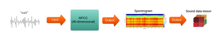
Abstract

      The advent of deep learning methods has led to significant improvements in speech recog-
nition. As a result, companies are concentrating more and more on taking advantage of these
progressive achievements and try to utilize speech recognition in their voice command systems.
However, data preprocessing, the size of the dataset and the architecture of the deep learning
model may have a huge impact on the accuracy of speech recognition and the best combination
of these arrangements is still unknown in different contexts. Therefore, in this study, we aim
to figure out whether it is possible and beneficial for companies to put an effort and use these
methods on relatively small datasets and in a language other than English (i.e. Dutch).
      In order to find the answer, we present a comparative study of two state-of-the-art speech
recognition architectures on small datasets to examine the practicality and scalability of these
academically well-received architectures in a real-life environment with all its limitations and
challenges. We conducted a series of experiments to train different network architectures on
different datasets. We realized that with the same data preprocessing and without using any
language model, the listen, attend and spell (LAS) model on both English and Dutch datasets
outperforms the CNN-BLSTM model. The LAS model achieved 32% character error rate
(CER) on LibriSpeech100 test-clean and 47% CER on the Dutch common voice dataset. Com-
paring the gained results in this research to the previously reported state-of-the-art results of
the LAS model, it can be deduced that the size of the dataset is significantly influential on the
accuracy of speech recognition systems. Moreover, considering the results of the experiments,
it is realized that the LAS model as an encoder-decoder attention-based deep learning approach
is also able to automatically recognize different languages. Further analysis also shows that the
training process of these models is quite resource-intensive and powerful processors (GPUs or
TPUs) are required in order to reach a reasonable accuracy level. This amount of resources
may not be available to all companies considering the budget restrictions. Therefore, although
the accuracy levels of the LAS-based models are enticing (both in English and Dutch), the
practicality of them in different environments can be considered controversial.
       Keywords: Speech recognition; deep learning; encoder-decoder networks; end-to-end
speech recognition; Dutch speech recognition; sequence-to-sequence; Speech-to-Text.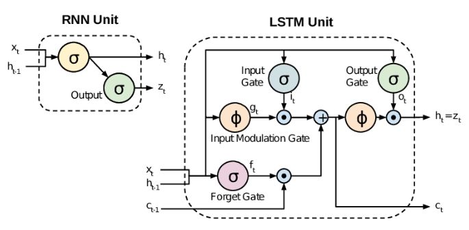
Acknowledgements

    I wish to express my sincere appreciation to my thesis advisor, Dr. M.A. (Marco) Wiering
at Groningen university, who has the substance of a genius: he convincingly guided and en-
couraged me to be professional and do the right thing even when the road got tough. He was
always available and responsible even though I was at a distance. Whenever I ran into a trouble
spot or had a question about my research or writing he helped me with his insightful guides.
He consistently allowed this project to be my own work but steered me in the right direction
whenever he thought I needed it. Without his persistent help, the goal of this project would not
have been realized.
    I would like to pay my special regards to Gijs van Wijk, Siamak Hajizadeh, Coenraad ter
Welle and Dr. Masoud Mazloom for their support and help. I am gratefully indebted to them
for their very valuable comments and supervision on this thesis.
    The physical and technical contribution of the company where I did my internship is truly
appreciated.
    I wish to express my deepest gratitude to my parents for providing me with unfailing sup-
port and continuous encouragement throughout my years of study and through the process of
researching and writing this thesis. This accomplishment would not have been possible without
their unconditional love.
    And finally, I want to dedicate this thesis to my source of strength and inspiration, Fouad.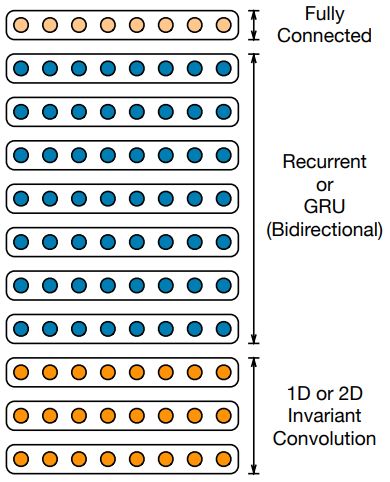
Contents

1   Introduction                                                                                                                                           6
    1.1 Introduction . . . . . . .     .   .   .   .   .   .   .   .   .   .   .   .   .   .   .   .   .   .   .   .   .   .   .   .   .   .   .   .   .   6
    1.2 Research Questions . . .       .   .   .   .   .   .   .   .   .   .   .   .   .   .   .   .   .   .   .   .   .   .   .   .   .   .   .   .   .   7
    1.3 Significance of the Study      .   .   .   .   .   .   .   .   .   .   .   .   .   .   .   .   .   .   .   .   .   .   .   .   .   .   .   .   .   8
    1.4 Thesis Layout . . . . . .      .   .   .   .   .   .   .   .   .   .   .   .   .   .   .   .   .   .   .   .   .   .   .   .   .   .   .   .   .   8

2   Theoretical Background                                                                                                                                 10
    2.1 Automatic Speech Recognition . . . . . . . . . . . . . . . . . . . . . .                                                           .   .   .   .   10
        2.1.1 Dutch Speech Recognition . . . . . . . . . . . . . . . . . . . .                                                             .   .   .   .   10
        2.1.2 Speech Recognition Applications . . . . . . . . . . . . . . . .                                                              .   .   .   .   11
    2.2 Recurrent Neural Networks (RNNs) . . . . . . . . . . . . . . . . . . .                                                             .   .   .   .   11
    2.3 Data Preprocessing . . . . . . . . . . . . . . . . . . . . . . . . . . . .                                                         .   .   .   .   12
        2.3.1 Zero Padding and Normalization . . . . . . . . . . . . . . . . .                                                             .   .   .   .   13
        2.3.2 Mel Frequency Filter Bank . . . . . . . . . . . . . . . . . . . .                                                            .   .   .   .   13
        2.3.3 One-hot Encoding . . . . . . . . . . . . . . . . . . . . . . . .                                                             .   .   .   .   14
    2.4 Components of the Attention-based Encoder-Decoder Models . . . . .                                                                 .   .   .   .   14
        2.4.1 Sequence-to-Sequence Models . . . . . . . . . . . . . . . . . .                                                              .   .   .   .   14
        2.4.2 End-to-End Models . . . . . . . . . . . . . . . . . . . . . . . .                                                            .   .   .   .   15
        2.4.3 Encoder-Decoder Framework . . . . . . . . . . . . . . . . . .                                                                .   .   .   .   15
        2.4.4 Attention Mechanism . . . . . . . . . . . . . . . . . . . . . . .                                                            .   .   .   .   16
        2.4.5 LAS Model . . . . . . . . . . . . . . . . . . . . . . . . . . . .                                                            .   .   .   .   17
    2.5 Components of the CNN-BLSTM Model . . . . . . . . . . . . . . . .                                                                  .   .   .   .   19
        2.5.1 Convolution-based Models . . . . . . . . . . . . . . . . . . . .                                                             .   .   .   .   19
        2.5.2 Pooling . . . . . . . . . . . . . . . . . . . . . . . . . . . . . .                                                          .   .   .   .   20
        2.5.3 Fully-Connected Layer . . . . . . . . . . . . . . . . . . . . . .                                                            .   .   .   .   21
    2.6 Literature Review . . . . . . . . . . . . . . . . . . . . . . . . . . . . .                                                        .   .   .   .   21
        2.6.1 Research Utilizing the LAS Model . . . . . . . . . . . . . . . .                                                             .   .   .   .   21
        2.6.2 Research Utilizing the CNN, LSTM or a Combination of Them                                                                    .   .   .   .   22
    2.7 Problem Statement . . . . . . . . . . . . . . . . . . . . . . . . . . . .                                                          .   .   .   .   23
    2.8 Justification of Choises . . . . . . . . . . . . . . . . . . . . . . . . . .                                                       .   .   .   .   24

3   Method                                                                                                                                                 25
    3.1 Research Pipeline . . .    .   .   .   .   .   .   .   .   .   .   .   .   .   .   .   .   .   .   .   .   .   .   .   .   .   .   .   .   .   .   27
    3.2 Datasets . . . . . . . .   .   .   .   .   .   .   .   .   .   .   .   .   .   .   .   .   .   .   .   .   .   .   .   .   .   .   .   .   .   .   27
        3.2.1 English Dataset      .   .   .   .   .   .   .   .   .   .   .   .   .   .   .   .   .   .   .   .   .   .   .   .   .   .   .   .   .   .   27
        3.2.2 Dutch Dataset .      .   .   .   .   .   .   .   .   .   .   .   .   .   .   .   .   .   .   .   .   .   .   .   .   .   .   .   .   .   .   29
    3.3 Implementation Details     .   .   .   .   .   .   .   .   .   .   .   .   .   .   .   .   .   .   .   .   .   .   .   .   .   .   .   .   .   .   29
    3.4 Evaluation Metrics . .     .   .   .   .   .   .   .   .   .   .   .   .   .   .   .   .   .   .   .   .   .   .   .   .   .   .   .   .   .   .   31
    3.5 Hardware Setup . . . .     .   .   .   .   .   .   .   .   .   .   .   .   .   .   .   .   .   .   .   .   .   .   .   .   .   .   .   .   .   .   31

                                                               2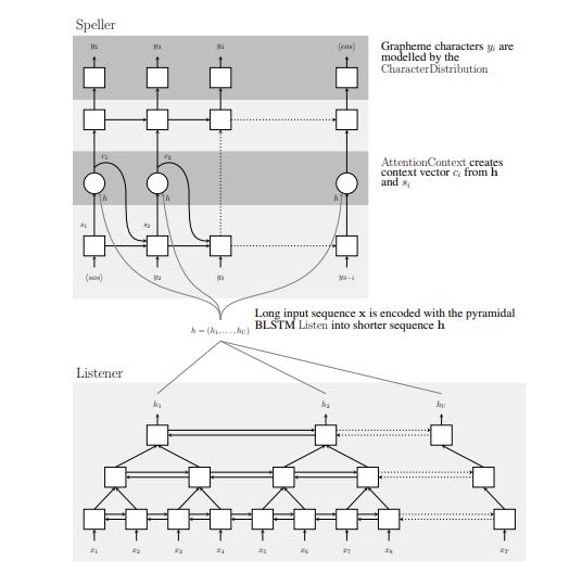
4   Experiments and Results                                                                                                           33
    4.1 Experiments . . . . . . . . . . . . . . . . .     .   .   .   .   .   .   .   .   .   .   .   .   .   .   .   .   .   .   .   33
    4.2 Results . . . . . . . . . . . . . . . . . . . .   .   .   .   .   .   .   .   .   .   .   .   .   .   .   .   .   .   .   .   36
        4.2.1 Results of the LAS Model . . . . .          .   .   .   .   .   .   .   .   .   .   .   .   .   .   .   .   .   .   .   36
        4.2.2 Results of the CNN-BLSTM Model              .   .   .   .   .   .   .   .   .   .   .   .   .   .   .   .   .   .   .   37
    4.3 Model Comparisons . . . . . . . . . . . . .       .   .   .   .   .   .   .   .   .   .   .   .   .   .   .   .   .   .   .   39

5   Discussion and Conclusion                                                                                                         40
    5.1 Discussion . . . . . . . . . . . . . . . . . . . . . . . .                .   .   .   .   .   .   .   .   .   .   .   .   .   40
         5.1.1 Resource Limitations . . . . . . . . . . . . . .                   .   .   .   .   .   .   .   .   .   .   .   .   .   41
    5.2 Conclusion . . . . . . . . . . . . . . . . . . . . . . .                  .   .   .   .   .   .   .   .   .   .   .   .   .   41
         5.2.1 Answers to the Supportive Research Questions                       .   .   .   .   .   .   .   .   .   .   .   .   .   41
         5.2.2 Answer to the Main Research Question . . . .                       .   .   .   .   .   .   .   .   .   .   .   .   .   42
    5.3 Future Work . . . . . . . . . . . . . . . . . . . . . . .                 .   .   .   .   .   .   .   .   .   .   .   .   .   43
List of Figures
2.1 Difference between RNN and LSTM units [48]. . . . . . . . . . . . . . . . . . . . . . 12
2.2 The pipeline of the data preprocessing. The sound waves are first transfered to the log-Mel filter
bank. After that, each text file is matched to its corresponding sound file as the label data. In
the next step, in order to make the labels understandable for machines, the sentences are cut to
characters and then a charachter to index table map is created. Then one-hot encoding is used to
. . . . . . . . . . . . . . . . . . . . . . . . . . 13
create target outputs for the networks.
2.3 The details of the data preprocessing. . . . . . . . . . . . . . . . . . . . . . . . . . 14
2.4 The one-hot encoded characters [1] . . . . . . . . . . . . . . . . . . . . . . . . . . . 14
2.5 Structure of a sequence to sequence model. The input "ABC" is mapped to the output "WXYZ".
It can be seen that the length of the input and the output are different [89]. . . . . . . . . . . 15
2.6 An encoder-decoder neural network. An example on machine translation: the input sequence is
in English and the output of the system would be in Korean [59]. . . . . . . . . . . . . . . 17
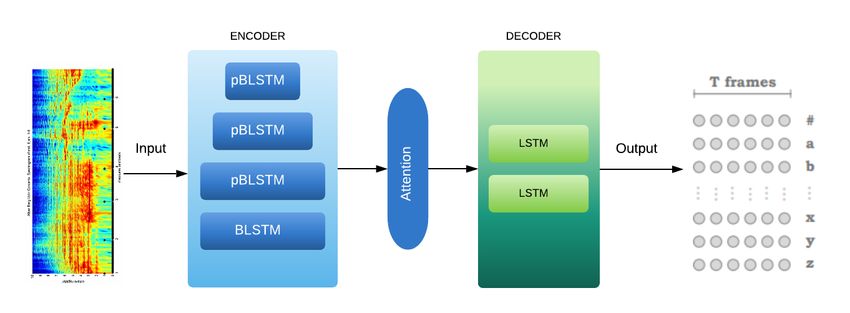
2.7 In figure (a) the LAS model’s components are shown. In figure (b) the structure
of the encoder-decoder is illustrated. . . . . . . . . . . . . . . . . . . . . . . . 18
2.8 The detailed structure of the LAS model’s pipeline from input to the output. . . . . . . . . . 19
2.9 Architecture of the DS2 system used to train on both English and Dutch speech [4]. . . . . . . 20
3.1 Deployment and management activities in CRISP-DM [91] . . . . . . . . . . . . . . . . 26
3.2 The pipeline of steps from starting the research to finding the best results . . . . . . . . . . 27
3.3 All the datasets that have been applied on two models in this research. The details of each
dataset are described in section 3.2. . . . . . . . . . . . . . . . . . . . . . . . . . . . 29
4.1 Character Error Rate (CER) and Loss of the LAS model on the Dutch dataset. The x axis is
the number of iterations and the y axis is CER/Loss rate. Pink is the validation CER, whereas
red describes the train CER. In the Loss graph, light blue represents the validation loss and dark
blue shows the training loss. . . . . . . . . . . . . . . . . . . . . . . . . . . . . . . 36
4.2 CER and Loss of the LAS model on the LibriSpeech100 dataset. Light blue is the validation
loss, whereas dark blue describes the train loss. Pink is the validation CER, and red describes
the train CER. The x axis is the number of iterations and the y axis is CER/Loss rate. . . . . . 37
4.3 CER and loss on the LibriSpeech100 dataset with 3CNN and 5BLSTM layers with the batch
size of 1. Light blue is the validation CER and dark blue describes the train CER. Red is the
validation loss, and orange describes the train loss. The x axis is the number of iterations and
the y axis is CER/Loss rate. At the best, it reached to the 0.83% CER. . . . . . . . . . . . . 38
4.4 CER and loss on the Dutch dataset with 3CNN and 5BLSTM layers with the batch size of 1.
Light blue is the validation CER and dark blue describes the train CER. Red is the validation
loss, and orange describes the train loss. The x axis is the number of iterations and the y axis is
CER/Loss rate. At the best, it reached to the 0.76% CER. . . . . . . . . . . . . . . . . . 38
4List of Tables
2.1 Papers which use a variation of the LAS as their base model on the different datasets in speech
recognition. The research of the pure LAS model on the LibriSpeech100 dataset has not been
done before. . . . . . . . . . . . . . . . . . . . . . . . . . . . . . . . . . . . . . 22
2.2 Papers that use models with the CNN, LSTM /BLSTM, or a combination of them on speech
recognition. Our study picked the Librispeech100 dataset and the CNN-BLSTM model structure. 23
2.3 The recent state-of-the-art researches on CNN-LSTM and encoder-attention-decoder models on
speech recognition on the LibriSpeech dataset since 2015. The numbers in parenthesis in the
WER column demonstrate if the results are from Librispeech960 or 100. In [104], the version
of the Librispeech data set has not been mentioned. . . . . . . . . . . . . . . . . . . . . 24
3.1 A list of English datasets for speech recognition. . . . . . . . . . . . . . . . . . . . . . 28
3.2 A list of Dutch datasets on speech recognition task. . . . . . . . . . . . . . . . . . . . . 29
4.1 Experiments which have been done on the LAS model to find the best hyperparameters on the
LibriSpeech100 dataset with the learning rate of 0.0001. Opt denotes optimizer, BS = batch
size, and Normalized denotes data normalization. The results are reported in character error rate
(CER). . . . . . . . . . . . . . . . . . . . . . . . . . . . . . . . . . . . . . . . 33
4.2 Experiments which have been done on the LAS model to study the effect of the different sizes
of datasets on the accuracy. Opt denotes optimizer, BS = batch size, DS means Dataset, and
Normalized denotes data normalization. The learning rate is equal to 0.0001. . . . . . . . . . 34
4.3 Experiments which have been done on the BLSTM model on the small-Libri dataset. The re-
ported CER is for the dev set. Max-pooling is used on top of the BLSTM layers. FC denotes the
fully connected layer and # BLSTMs shows the number of BLSTM layers. No CNN layers used
in these experiments. Init. represent weight initialization which prevents exploding or vanishing
of the layer activation outputs. In this thesis random and Kaiming initializaion is used. . . . . 34
4.4 Experiments which have been done on the CNN-BLSTM model on the small-Libri dataset. The
reported CER is for the dev set. ReLU has been used after the BLSTM layers on top of the Max-
pooling and the fully-connected is the final layer. In the BLSTM layers, the hidden dimension
of each direction is equal to 256. FC denotes the fully connected layer with the dimension of 30,
# CNNs shows the number of CNN layers and # BLSTMs shows the number of BLSTM layers
used in the architecture and Init. represent data initialization. . . . . . . . . . . . . . . . . 34
4.5 Experiments which have been done on the CNN-BLSTM model on different dataset. According
to the results of previous experiments the initialization is Kaiming. ReLU has been used after
the BLSTM layers on top of the Max-pooling and the fully-connected is the final layer. FC
denotes the fully connected layer, # CNNs shows the number of CNN layers and # BLSTMs
shows the number of BLSTM layers used in the architecture. . . . . . . . . . . . . . . . . 35
4.6 The summary of the best results of all the experiments which have been done with both models
on the Dutch and LibriSpeech100 datasets. The Batch size is set to 1.. . . . . . . . . . . . 35
4.7 The target and the output of the LAS model on the Dutch dataset. . . . . . . . . . . . . . . 37
4.8 The target and the output of the LAS model on the LibriSpeech100 dataset. . . . . . . . . . 37
5Chapter 1
Introduction
1.1 Introduction
Speech is the most natural form of human communication [101]. On average people speak
150 words per minute, while they type on average about 50 words per minute, approximately
one-third [3]. This shows that we can communicate faster and convey more information via
speech than with text. This motivated humans to crave for building machines that are able
to recognize our speech more accurately and to make them better at communicating with us
[3]. Such machines are called spoken dialogue systems and are developed to interact with
humans [60]. Other words such as voice command systems and conversational AI have also
been proposed to describe these machines, but in this report we use the term spoken dialogue
systems. Moreover, another common term that emerged when such machines became prevalent
was automatic speech recognition (ASR) which refers to the process of converting the speech
signal into its corresponding text [56].
Nowadays, companies are aware of the significance of speech in the conversation and want
to increase the quality of communication with their costumers. However, in the 30 years history
of the spoken dialogue systems, the accuracy of speech recognition was not high enough to
be trusted as an alternative to humans. Therefore, using a spoken dialogue system was not
in the center of the companies’ attention in order to invest in. Only during the past decade
some initiatives reached some acceptable accuracy rates and put the speech recognition in
the limelight again. The history of the voice command systems can be divided into three
generations: symbolic rule or template-based (before the late 90s), statistical learning-based
(from 90s till 2014), and deep learning-based (since 2014) [26]. It was just after the advent of
the deep learning in speech recognition tasks that companies also got attracted to the use of such
a system in their business lines. By utilizing deep learning, speech recognition became accurate
enough to be useful in the real-life and business use cases [53]. Recently, speech recognition,
as the first step of the human-computer conversation system has attracted increasing attention
due to its potentials and enticing commercial values.
With the increased need for having better communication with the customers, many com-
panies feel the urge to at least experiment with the voice command systems based on the stag-
gering adoption rate of such systems in countries like the US and China. According to the
Gartner, by 2021, 15% of all customer service interactions will be completely handled by AI
1 . There is another survey which shows that 87% of the participants with the role of retailers
believe that conversational AI will lead to higher satisfaction levels in their business lines 2 .
Despite all the efforts and improvements in speech recognition, it is still hard to reach a
1 www.gartner.com/smarterwithgartner/4-trends-gartner-hype-cycle-customer-service-customer-engagement/
2 www.letslinc.com/wp-content/uploads/2017/07/Lin_Brand-Garage_Customer-Service-and-AI-Report.pdf
6100% accuracy due to several factors. Such factors make it difficult for machines to recog-
nize and fully understand human speech. For instance, due to the variability in the speech
signal, the analysis of human speech which is considered as continuous speech is a challeng-
ing task for machines [26]. Although there has been a huge improvement in English speech
recognition, enhancement is still needed for other languages. The Dutch language is not an
exception. The success of speech recognition in one language does not necessarily extend to
the other languages. Therefore, in this research, we try to apply a speech recognition system
in one of the business lines of a Dutch financial company in order to assess the claims of the
scholars. The results can be used in order to improve the effects of speech recognition on the
Dutch company’s customer features. After all, one of the main advantages of acquiring speech
recognition in a business is the reduction of human resources in customer service which leads
to lower employee costs. Moreover, a personalized voice assistant could increase loyalty and
customer satisfaction [95].
Studies show that in the topic of ASR, deep learning has shown to be a successful contribu-
tion [44]. Generally, the main focus of research in deep learning is to design better network ar-
chitectures, such as: deep neural networks (DNNs) [23], convolutional neural networks (CNNs)
[55, 79], recurrent neural networks (RNNs) [39], and end-to-end models [8, 14, 37]. Among all
of these aforementioned network structures, the focus of this research is on the CNNs, RNNs,
and end-to-end encoder-decoder networks and the crucial components in these deep learning
systems will be discussed. These components are the model architecture, large labeled training
datasets, computational scale, data preprocessing, and hyperparameter settings. The effect of
these components on the accuracy of speech recognition will be described as well.
In particular, this work will be supported by the experimental investigation of the func-
tional accuracy of neural networks on speech recognition tasks. We also conduct numerous
experiments with two different neural network models to predict speech transcriptions from
audio.
From a high-level view, the final goal of this research is to pave the way for designing a
scalable and practical speech recognition model which considers the limitations in the real-life.
A model from which both users and companies can benefit.
1.2 Research Questions
The main objective of this thesis is to first find the two most acclaimed and accurate deep learn-
ing architectures for speech recognition tasks on the English dataset, and then, to investigate
the effect of the size of the training datasets on the accuracy and the performance of the mod-
els. Finally, the models will be applied to the Dutch dataset. In the end, by scrutinizing the
results of the experiments, some of the significant factors which may influence reaching higher
accuracy can be characterized.
The conversational agent at the first step should correctly understand the customers’ ques-
tions and then answers them in a reliable and convenient way. To achieve such a system the first
step is having an accurate speech recognition system. In the literature, different deep learning
methods have been applied to understand and recognize the user’s utterances and they achieved
high accuracy in speech recognition tasks [67, 15, 42].
Research Objective: The main objective of this research is to help Dutch organizations
to choose the best deep learning architecture based on the available resources and datasets at
hand.
To support the main objective, this thesis attempts to address the main research question
(MRQ) followed by three supportive research questions (SRQ):
71. MRQ: "Which deep learning architecture for speech recognition tasks performs best on
relatively small Dutch datasets"
(a) SRQ1: What are the two most used, state-of-the-art deep learning architectures for
speech recognition tasks?
To answer this question, the literature will be investigated to find two state-of-the-
art network structures for speech recognition tasks. Among all the networks, we
will pick those two architectures which have been used the most in order to have
more literature available to compare the results.
(b) SRQ2: What are freely available datasets in English and Dutch languages for
speech recognition tasks?
This question will be answered by searching for the datasets for speech recognition
tasks in English and Dutch languages.
(c) SRQ3: What are the effects of the size of the dataset on the accuracy of the state-
of-the-art models?
Analyzing the results of the experiments and comparing them with the literature
will specify if the models are sensitive to the size of the datasets or not.
By answering the three supportive questions separately, we will be able to answer the main
research question. Some experiments will be conducted to apply both of the models on the
selected English and Dutch datasets. By comparing the results of the experiments on both
models the more accurate model will be found. Moreover, in order to fulfil the objective of
this thesis, we will find out if the more accurate model on the English dataset can achieve high
accuracy on the Dutch dataset as well.
1.3 Significance of the Study
The main contribution of this thesis is to examine the practicality of the two most commonly
used state-of-the-art deep learning architectures in the real-life environment with a limitation
on the processing power and also a limited accessible dataset. These resources have been
provided to us for this research by a Dutch financial company with near 20,000 employees.
In the literature, state-of-the-art models are trained on big datasets such as LibriSpeech960h,
Google voice search with 2000 hours of speech, Baidu dataset, etc. However, the obstacles of
having limited resources in the real world are usually not considered by scholars. Through this
research, we want to investigate if reaching such accuracy is achievable using the resources
available to the companies. Otherwise, although these models are reported to be able to give
us a very high accuracy but using them in a company can not be possible and there will be a
constant need for big companies like Google or Baidu to provide the speech recognition service
to other companies because of their huge dataset and very high processing power.
1.4 Thesis Layout
The rest of this thesis will be structured as follows. The next chapter will describe the theo-
retical background of the relevant methods and models in the speech recognition task. Here
some explanations will be provided on the details of the models used throughout this thesis. In
chapter 3 the methodologies are discussed, explaining the selection of datasets, together with
implementation details and experiments. In chapter 4, the experimental setup to address the
research questions will be described. Section 4.2 contains the results of these experiments and
8the elaboration on the possible reasons behind them. Finally, in chapter 5 the research ques-
tions are addressed and the conclusions drawn from the experiments together with potential
future work are presented.
9Chapter 2
Theoretical Background
2.1 Automatic Speech Recognition
Speech recognition is the first ability which an artificial intelligence (AI) system needs in order
to have a smooth human-like conversation with a human. Speech recognition can detect the
human voice and convert speech into text which is some form of computer-readable data [86].
This research is in continuation of the previous works in the field of deep learning for speech
recognition. In the field of ASR with more than 60 years of research history [57, 25, 9], speech
recognition has always been a difficult task. The complication in speech recognition leads to
the complexity of the language understanding components and may also affect the efficiency of
spoken dialogue systems [13]. Errors in speech recognition limited the capabilities of spoken
language understanding and made the text-based language understanding more in the center
of attention [94] rather than speech. Therefore, in order to give ASR systems the value that
it actually has in human communication, it is important to increase the accuracy of speech
recognition. To have accurate speech recognition, applying some deep learning techniques
helped to achieve huge successes in the field [57]. It has been more than 20 years that feed-
forward neural network acoustic models were explored [73, 30, 11]. Consequently, the number
of applications in speech recognition has increased sharply. Speech recognition consists of
three main sections; signal level, acoustic level, and language level. In the signal level, the
aim is to extract features from the signal by doing pre-processing and denoising (if needed).
This step is common in most of the machine learning tasks. The acoustic level is responsible
for the classification of the features into different acoustic states which provide more precise
criteria. In the language level, we try to create meaningful sentences based on words which are
the combination of different sounds [12].
2.1.1 Dutch Speech Recognition
There are a couple of services and open source projects which work on Dutch speech recog-
nition. There are services such as Google cloud speech-to-text, Speechmatics, Nixidia, and
open-source Kaldi project. However, at the time of writing this report, Google’s specialized
model for phone conversations is not available in Dutch. The accuracy of the Nixidia is not
satisfying enough and the Speechmatics is costly [96]. Therefore, for the companies, especially
those who work with confidential data, it is better to create their own Dutch speech recognition
system. One reason is that due to the higher availability of English datasets, most of the avail-
able systems are not as accurate as they are in English. Moreover, by having their own speech
recognition system, companies can have full control over the data. Although there are some
rules which say Google is not allowed to use the audio data for its own projects unless this per-
10mission has been given to Google, the data still has to be sent over. Furthermore, in order to use
their professional phone model, Google asks for the audio data as well. Therefore, it sounds
more secure and peaceful to keep everything in-house especially with the new GDPR laws in
place [96]. Therefore there is a need for building a more accurate Dutch speech recognition
system which is also applicable for the companies to use and customers will benefit from it as
well.
2.1.2 Speech Recognition Applications
The technology of speech recognition and using digital assistants have rapidly moved from
cellphones to the homes and offices, and its application in different industries such as banking,
marketing, travel agency, and healthcare is becoming apparent. Here are some of the applica-
tions in which speech recognition is used as one of the main components [10]:
• At the office
1. Search for documents on the computer
2. Request for printing
3. Start video conferences
4. Schedule meetings
• Banking
1. Request information about the account balance and transactions history
2. Payments
3. Ask mortgage related questions
4. Customer intention analysis
• Medical
1. Immediate, hands-free information retrieval
2. Payments
3. Fast and targeted access to the required information
4. Repeating processes and the steps of specific instructions
5. Effective way for entering the data and information
By utilizing speech recognition in these areas, we can see the prominent potential in speech
recognition to increase the efficiency of all these areas and it can be very effective in many
other industries as well.
2.2 Recurrent Neural Networks (RNNs)
Recurrent neural networks or RNNs [76] are a class of neural networks where connections
between nodes form a directed graph along with sequential data. As a result, RNNs are able
to exhibit temporal dynamic behavior. RNNs use their internal state (memory) to process se-
quences of inputs. They can be considered as neural networks with loops. Therefore, RNNs are
a natural choice for processing sequential data of variable length. Due to their internal memory,
RNNs are able to remember previous inputs while taking in new input. This memory structure
makes the RNNs a perfect predictor of what will come next. By utilizing memory, RNNs have
11a deeper understanding of sequences compared to other algorithms [28]. As a result, RNNs are
the preferred algorithm for those Machine Learning (ML) problems like time series, speech/text
recognition, financial data, audio, etc. The short-term memory of RNNs comes from the recur-
rency which helps the network to remember the past [2]. Deep neural networks (DNNs) are
dominant in many ML tasks because of their high-performance [85]. However, for sequential
data like Natural Language Processing (NLP), machine translation [89] or speech recognition,
RNNs and especially Long-Short-Term Memory (LSTM) networks perform better [45]. In the
naive RNN implementation, the input will not remain in the memory for a long time [66] and
the gradients may either increase or decrease exponentially over time depending on the largest
eigenvalue of the state-update matrix. Thus, it is hard to train such a network. To overcome
this problem, LSTMs are used [33]. The difference between a simple RNN unit and an LSTM
unit is shown in figure 2.1. The LSTM also shows better results compared to fully-connected
feed-forward DNNs [92]. So far, LSTMs have been effective for learning sequence mappings
in speech recognition [40]. They are commonly built as a pipeline of the ASR component to
transcribe the user’s speech to text. One of the conventional RNNs downsides is that they can
only use the previous context. However, in speech recognition, we need the whole utterance to
be transcribed at once which increases the need of exploiting future context. To do this, bidirec-
tional RNNs (BRNNs) are used to process the data with two hidden layers in both directions.
The data then feeds forwards to the same output layer. BLSTM is the combination of BRNNs
with LSTM which make it possible to access long-range context in both input directions [40].
Apart from all the advantages of BLSTM networks, the disadvantage of BLSTM acoustic mod-
els is that they need more tuning to their training compared to feed-forward neural networks.
Figure 2.1: Difference between RNN and LSTM units [48].
2.3 Data Preprocessing
After attaining the data, data preprocessing is the first step in speech recognition. The general
work of speech recognition is to take the sound signals as inputs and create the characters as
the output. Sound waves are one-dimensional. At every moment in time, based on the height
of the wave, the sound waves have a single value. However, these waves should be changed
into numbers to be understandable for computers. Therefore, in a process named as sampling,
only the height of the wave will be recorded at equally-spaced points. Based on the Nyquist
theorem, which suggests to sample a sine wave at least twice the sample frequency, it is now
12possible to reconstruct the original sound wave from the spaced-out samples perfectly without
losing any data [21]. In this research, the format of the voice signals has been converted from
.flac into .wav files. Then the log-Mel filter bank extracts features from the signals and creates
the spectrogram of each sound file. In this research, a 40-dimensional log Mel-frequency filter
bank feature with a window size of 0.025 has been extracted from the raw speech data with
delta and delta-delta acceleration. As a result, from the spectrograms made from the Mel-
frequency filter bank, tensors of the sound data will be created. For labeling the sounds, a text
file corresponding to each sound file is provided in the dataset. Each text file has been separated
character by character. Then a character map is created which maps each character to a number
so that we can easily map them to the One-Hot encoding system. Figure 2.2 demonstrates the
whole process for the data preprocessing in this research.
Figure 2.2: The pipeline of the data preprocessing. The sound waves are first transfered to the log-Mel filter
bank. After that, each text file is matched to its corresponding sound file as the label data. In the next step, in order
to make the labels understandable for machines, the sentences are cut to characters and then a charachter to index
table map is created. Then one-hot encoding is used to create target outputs for the networks.
2.3.1 Zero Padding and Normalization
Zero padding is a crucial feature to increase the width of the input and make it wider. In general,
zero padding is used to control the input width and the size of the output consequently [34]. In
this research, all the sound sequences are padded to a max length so that the width of all the
input data becomes unified. For the normalization, the input feature sequence H is normalized
as follow:
H −µ
H0 = (2.1)
σ
where µ and σ are vectors of per feature channel means and standard deviation over all of these
feature channels. To explain more, the mean is the sum of all input data divided by the total
number of them as shown in equation 2.2.
1
µ= Hi (2.2)
m∑i
and the standard deviation as shown in equation 2.3, demonstrates to what extent a set of
numbers are different from each other [34].
r
∑i (Hi − µ)2
σ= (2.3)
m
2.3.2 Mel Frequency Filter Bank
The Mel (Melody) scale was first suggested by Stevens and Volkman in 1937 [87]. A Mel
frequency filter bank is suitable for speech recognition tasks because it considers the sensitivity
of humans to a specific frequency. It is computed by converting the conventional frequency to
Mel Scale. This manipulation helps to understand the human voice better. Based on a linear
cosine transform of a log power spectrum on a nonlinear Mel scale of frequency, the Mel
13frequency cepstrum (MFC) can represent the short-term power spectrum of a sound [78]. On
top of the fast Fourier transform (FFT) on the magnitude spectrum, a filter bank will be used to
derive the MFC feature.
In figure 2.3 the process from the sound wave to the tensor data has been illustrated.
Figure 2.3: The details of the data preprocessing
2.3.3 One-hot Encoding
When there is a classification problem, the one-hot encoding can be used. By using one-
hot encoding, categorical variables are converted into an ML friendly form so that the ML
techniques have easy access to the target output. In figure 2.4 the conversion from characters
to one-hot encoded numbers is shown. It can be seen that the character "A" has the same value
(1000) in different positions.
Figure 2.4: The one-hot encoded characters [1]
2.4 Components of the Attention-based Encoder-Decoder Models
Here, the essential components of the end-to-end encoder-attention-decoder models will be
described.
2.4.1 Sequence-to-Sequence Models
Despite all the advantages of DNNs, they have a significant limitation. They can only be
applied when the inputs and desirable output can be sensibly encoded with fixed-dimension
vectors. However, there are many problems like speech recognition and machine translation in
which the length of the sequences is not known a-priori. In speech recognition, for instance,
the network should learn to transcribe an audio sequence signal to a text word sequence [15].
In such problems, a sequence of input should match to a sequence of outputs. Therefore, a
domain-independent method that learns to map sequences to sequences is needed [89]. A se-
quence to sequence model is a framework that tries to address the problem of learning variable-
length input and output sequences. Such a model could be an LSTM sequence-to-sequence
model which is a type of neural generative model [89]. It uses an encoder-decoder structure to
first map the sequential variable-length input into a fixed-length vector by an RNN encoder and
14then in the RNN decoder, this fixed-size vector will be used to produce the variable-length out-
put sequence, one token at a time [15]. In figure 2.5 the structure of a sequence to a sequence
model has been illustrated.
Figure 2.5: Structure of a sequence to sequence model. The input "ABC" is mapped to the output "WXYZ". It
can be seen that the length of the input and the output are different [89].
2.4.2 End-to-End Models
An end-to-end model in speech recognition, simply means "from speech directly to transcripts"
[15]. In general, it denotes a simple single model that can be trained from scratch, and usu-
ally directly operates on words, sub-words or characters/graphemes. Accordingly, it simplifies
the decoding part by removing the need for a pronunciation lexicon and the whole explicit
modeling of phonemes [105]. The neural network then provides a distribution over sequences
directly. All speech recognition systems with an end-to-end neural network, utilize RNNs in at
least some part of the processing pipeline [106]. Since the most successful RNN architecture
used in speech recognition is the LSTM [39, 35, 45, 97], LSTMs have become a default method
for end-to-end models.
2.4.3 Encoder-Decoder Framework
In general, an encoder-decoder is a neural network that learns a lower-dimensional representa-
tion of the original data. It can be considered as a multi-layer PCA (a dimensionality reduction
technique) with non-linearities. The main idea of the framework is to divide the process of gen-
erating output into two subprocesses; encoding phase and decoding phase. The encoding part
is responsible for providing a good representation of the input. To do so, a projection function
also known as "encoder", should project the input into another space like in a feature extraction
process. It extracts a feature vector from the input. Now that the encoder generated a "latent
vector", it will pass this vector to the decoder. The decoder then processes the extracted feature
vector and creates the output based on this vector which although it is smaller than the input, it
contains the most important features and information of the input. Both encoder and decoder
have a neural structure. However, the structure of the encoder could vary according to the type
of input. For instance, for text or other sequential input data, an RNN is used as the encoder,
but CNNs can also be used to encode the images [5]. The neural encoder-decoder framework
has recently been applied as a solution to a wide variety of challenges in natural language pro-
cessing, computer vision and speech recognition. This framework can enhance the accuracy
of speech recognition task significantly [105, 15, 8]. More specifically, the encoder-decoder
structure is usually used when the goal is to generate sequential outputs such as text.
One of the main problems of decoders in the encoder-decoder based models is extracting
long-term dependencies and generating different sentences. A simple solution to this is using
LSTM cells. Another approach is to make deeper decoders by using stacked structures of
RNNs. As a result, the model will be able to generate more detailed sentences. However, using
stacked decoder structures may cause the problem of vanishing gradients. To avoid this, an
15attention mechanism can be used. The attention mechanism is a technique to focus on different
parts of the input, at each step of generating outputs.
The encoder-decoder framework with attention has become the standard approach for ma-
chine translation [7, 102], object recognition in images [6] and speech recognition [15, 93].
In this work, we also investigate the LAS model which is an encoder-attention decoder based
model for speech recognition on the Dutch dataset.
2.4.4 Attention Mechanism
Generally, the attention mechanism was developed to improve the performance of RNNs in
the encoder-decoder framework. It is an increasingly popular mechanism used in many neural
architectures [32]. In speech recognition, it is important to process elements of the sound wave
correctly. These elements are being characterized by having a different relevance to the task at
hand. For instance, in a visual question-answering task, objects in the foreground are usually
more relevant in answering a question but background pixels are more relevant to questions
regarding the scenery. An effective solution to such problems is to find the relevant part so
that the system could provide the computational resources efficiently on a restricted set of
important elements. This solution is viable, especially if the input is very information-rich, like
in speech recognition, where the input is possibly a long audio sequence. There is a machine
learning-based approach which tries to find the relevance of input elements by automatically
weighing the relevance of any region of the input, and then taking such a weight into account
while performing the main task. The attention mechanism is the most common and well-
known solution to this problem [32]. Bahdanau, Cho, and Bengio were the first researchers to
introduce the attention mechanism in their research on natural language processing (NLP) for
machine translation tasks [7].
In the encoder-decoder approach, the encoder should compress all the important informa-
tion of the source sentence into a fixed-size vector. This may cause difficulty for the neural
network to model long sentences, especially those that are longer than the sentences in the
training corpus [7]. The advantage of applying attention from the baseline encoder-decoder is
that it does not attempt to encode the input sequence into a single fixed-size context vector. In-
stead, it encodes the input into a sequence of annotated context vectors that are filtered for each
output time step specificaly. Then, it selects a combination of these vectors while decoding and
generating the output in each step.
The attention mechanism addresses both alignment and translation. Alignment is about
matching which parts of the input sequence are relevant to each word in the output and by
using translation the network tries to highlight the relevant information to select the appropriate
output. To find the appropriate output, a distribution function is used which takes into account
locality in different dimensions, such as space, time, or even semantics. It is also possible
to model attention in such a way that it will be able to compare the input data with a given
pattern, based on similarity or significance. However, an attention mechanism can learn the
concept of relevant information by itself, consequently, it can create a representation to which
the important data should be similar [32]. As a result, by injecting knowledge into the neural
model, attention can also play a role in addressing fundamental AI challenges.
In figure 2.6 the structure of an encoder-decoder framework with attention mechanism is
demonstrated.
16Figure 2.6: An encoder-decoder neural network. An example on machine translation: the input sequence is in
English and the output of the system would be in Korean [59].
Interestingly, attention has two positive effects: it improves the performance of the network,
and interprets the behavior of neural networks which are hard to understand [41]. Understand-
ing the behavior of neural networks is difficult because the outputs are numeric elements that
do not provide any means of interpretation by themselves. Attention helps this challenge by
computing the weights and providing relevant information about the results of the neural net-
work. Therefore, it is able to explain the ambiguity in the output of the neural network [32].
In general, the RNN encoder-decoder model with attention provides good results in speech
recognition.
2.4.5 LAS Model
The LAS model is an attention-based encoder-decoder neural network which tries to learn how
to create the transcript of an audio signal, one character at a time. There are also some other
approaches such as connectionist temporal classification (CTC) [36] and sequence-to-sequence
models with attention [7]. However, there are some limitations to using them. CTC is a neural
network output and scoring algorithm, for training sequence-to-sequence models to tackle se-
quence problems where the timing is variable and the length of the input and output sequences
are not equal [29]. Label outputs in CTC are assumed to be conditionally independent of each
other. Moreover, in the sequence-to-sequence approach, only the phoneme sequences have
been taken into account [18, 19].
Unlike previous state-of-the-art approaches that separate acoustic, pronunciation, and lan-
guage modeling components and train them independently [83], the LAS model attempts to
rectify this disjoint training issue by using the sequence-to-sequence attention-based encoder-
decoder learning framework [18, 19, 89].
The LAS model includes an encoder as a listener and a decoder as an attender and speller.
The encoder consists of two pyramidal BLSTM (pBLSTM) layers that convert low-level speech
signals into higher-level features. The speller is an attention-based character decoder that uti-
lizes these higher-level features and produces the output as a probability distribution over se-
17quences of characters using the attention mechanism [18, 19]. The listener and the speller are
trained jointly. Figure 2.7a demonstrates the three modules in the LAS model. Moreover, Fig-
ure 2.7b illustrates the pyramidal model in the LAS model with its two components. As it can
be seen in the picture, in the decoder, the teacher forcing is also used. It means that the output
of the previous layer is given to the current layer of the decoder as the input [100].
(a) Components of the LAS (b) The listener in the LAS model is a pyramidal BLSTM
end-to-end model [16] encoding the input x into high level features h, the speller is
an attention-based decoder producing the y characters from
h [15]
Figure 2.7: In figure (a) the LAS model’s components are shown. In figure (b) the structure of
the encoder-decoder is illustrated.
Structure of the LAS Encoder
The encoder uses a BLSTM [38] with a pyramid structure. This pyramidal structure reduces
the length of h (a high-level representation of the input x). Due to the difficult process of the
decoder extracting the relevant information from a large number of input time steps, a simple
BLSTM converged very slowly. Therefore, using a pyramid BLSTM (pBLSTM) is helpful,
since it reduces the temporal dimension of the decoder, which results in less computational
complexity [15]. As a result, the attention model will be able to extract the relevant information
in a smaller number of time steps. Moreover, based on the deep architecture of both the listener
and speller, the model is able to learn nonlinear feature representations of the data.
Structure of the LAS Decoder
The second part of the model is the decoder. In the decoder, an attention-based LSTM trans-
ducer is used. At each step of the output, the transducer generates a probability distribution
over the next characters conditioned on all the characters seen previously and the given en-
coder vector.
In this research, the log-Mel spectrogram is passed as the input through an encoder with
three layers of pBLSTMs with a cell size of 256 on top of a BLSTM layer to yield a series
of attention vectors. The attention vectors are fed into two layers of LSTMs with the cell
18dimension of 512, which yields the tokens for the transcript. At the end, the output text is
evaluated using character error rate (CER) metrics. Figure 2.8 demonstrates the LAS model
which has been implemented in this project. We used the exact structure as explained in [15].
Figure 2.8: The detailed structure of the LAS model’s pipeline from input to the output.
2.5 Components of the CNN-BLSTM Model
2.5.1 Convolution-based Models
Due to the promising reported results of DNNs, almost all state-of-the-art ASR models in the
literature use a variation of DNNs [23, 24, 44, 62, 50, 103]. For instance, RNNs and more
specifically LSTMs, are more recently being used in the state-of-the-art speech recognition
systems [39, 83, 84]. Moreover, deep LSTM networks have shown better performance com-
pared to the fully-connected feed-forward DNNs in speech recognition tasks [4, 14, 16, 70].
Apart from RNNs, using CNNs is also an option for sequence learning tasks, such as speech
recognition [58]. The combination of RNNs and CNNs has also shown accurate results in
speech recognition [74, 98].
Based on the study in [106], CNN-based end-to-end speech recognition frameworks have
shown promising results on the TIMIT dataset. Based on this capacity of the model, in this
research, we decide to use CNNs and see how the results will be in the speech recognition task
on the Librispeech100 and the Dutch dataset. To efficiently scale our model, in this project dif-
ferent numbers of convolutional layers are added before the BLSTM layers to see how deeper
CNNs will affect the accuracy of the speech recognition task [4, 14, 16, 70]. In [43], they also
use a deeper CNN in a visual recognition task and benefit from it. Moreover, following the re-
sults of the previous research [39], to increase the accuracy we build a hierarchical architecture
and added more hidden layers to the networks and made it deeper, rather than making each
layer larger.
It has been found that for the feature extraction, the combination of LSTMs together with
convolutional layers give a very good result. In [82] and [42], researchers could reach state-
of-the-art results by using this combination of CNNs and LSTMs. Using CNNs in addition to
RNNs resulted in better network architectures and proved to be efficient, especially to facilitate
efficient training. Consequently, this architecture improves the key components of sequence-
to-sequence models [77].
In this research, we followed the architecture which has been used in [4]. The model starts
with one or more convolutional layers, after that one or more recurrent layers are added, and
one fully connected layer will be the last layer of the network. Figure 2.9 demonstrates the
19architecture of this model.
Figure 2.9: Architecture of the DS2 system used to train on both English and Dutch speech [4].
Studies reveal that using a stack of BLSTM and max-pooling layers in natural language
inference yields state-of-the-art results [90, 22]. Therefore, we use a deep BLSTM structure
and after each layer, we optionally add the max-pooling layer in the time dimension to reduce
the input’s feature-length.
Given a sequence of T words (w1 ..., wT ) as the input, the BLSTM layer gives a set of
vectors (h1 , ..., hT ) as the output. Each ht ∈ (h1 , ..., hT ) is the concatenation of a forward and
backward LSTM layer in the BLSTM. The output dimension of the max-pooling layer is the
same as ht . For each dimension, max-pooling returns the maximum value over the hidden units
(h1 , ..., hT ) [90].
2.5.2 Pooling
Pooling uses local summary statistics to summerize the output feature maps over a region.
The summarization is done within a local neighborhood like in convolution [34]. Here are the
common pooling operations:
• Max pooling: returns the maximum activation among rectangular neighbors.
• Average pooling: returns the average activation among rectangular neighbors.
Due to its regional summarization, usually fewer pooling operations are used, compared to
convolution. Pooling is a technique for downsampling the input data. For instance, max-
pooling with a window size of three with a stride of two can summarize the three activations of
an input and its neighbors into one summary statistic. In fact, with a pooling with a stride of s,
the feature map is downsampled with a factor of s.
Moreover, some advantages of pooling are that it is invariant to small translations and it
does not need any parameters to be trained [34]. The only thing that is important in pooling
are the values within its pooling window. This means that the location of the neighbors in
the window has no effect on this process. Although small translations of the input may cause
shifting in the activation in the feature maps, they may still fall within the same pooling window.
This is very useful in speech recognition where matching the label to the sound wave could be
tricky. Pooling also uses a parameter offset. Different input sizes can be managed by varying
20the offset of pooling windows, such that the resulting output will always be the same size before
the classification layer.
In this research max-pooling in the time-dimension has been applied. In the structures with
two layers of BLSTM, max-pooling has been applied between the two BLSTM layers as it
was done in [15]. But when the number of BLSTM layers is more than two, max-pooling is
positioned at the end of all the BLSTM layers and before the ReLU to prevent more reductions
in the time-dimension.
2.5.3 Fully-Connected Layer
As traditionally seen in standard feed-forward Neural Networks, the final features from mul-
tiple convolutions, BLSTMS and pooling are flattened and fed to the fully-connected layers
[34]. Convolutional layers work as feature extractors and the fully-connected layers map the
features to classes. Both are trained at the same time with the same training procedure. The
output of the fully-connected layer as the final layer is 30 scores (one for each letter in the En-
glish dictionary) plus the apostrophe, silence (#), and two special characters for the encoding
of duplications (once or twice) of the previous letter known as special “repetition” graphemes.
2.6 Literature Review
Generally, deep learning led to an enhancement of speech recognition. Among all the various
deep learning architectures, CNN-LSTM based and end-to-end models are dominant in the
literature due to their promising results. End-to-end models combine the acoustic model (AM),
language model (LM) and an acoustic-to-text alignment mechanism which leads to a simpler
ASR system [15, 49]. In addition, the combination of CNN and LSTM layers also work well
for the feature extraction [82].
Here, more details about the CNN-LSTM model and the LAS model as a well-known,
state-of-the-art architecture among all the encoder-attention-decoder models will be discussed.
2.6.1 Research Utilizing the LAS Model
The authors of [61] applied the LAS model with sub-word units. They use an extended pre-
training procedure where besides increasing the encoder depth, the hidden-layer dimension of
the LSTMs is grown as well. The model starts with two layers of 512 dimensions in the encoder
and increases to six layers with a dimension of size 1024. Moreover, the first pre-training step is
done without dropout. Then they tune the curriculum learning schedule and improve upon that
model. The researchers in [61] work on LibriSpeech100 and get the word error rate (WER)
of 14.7% on the test-clean variant. However, on LibriSpeech 960, the performance is 4.8%
WER in test-clean. In [105], an end-to-end, encoder-attention-decoder model is implemented
in which a deep BLSTM network is the encoder and LSTM layers form the decoder. In the
encoder, they use max-pooling after every layer in the time dimension in order to decrease the
length of the encoder. Therefore, we also decided to use max-pooling in our CNN-BLSTM
model structure. Moreover, the RWTH extensible training framework for universal recurrent
neural networks (RETURNN) is used in [105] as the pre-training process. RETURNN is an
optimized implementation for fast and reliable training of RNNs on multiple GPUs based on
Theano/TensorFlow [27].
The model is tested on LibriSpeech 1000h and the reported performance is 4.87% WER.
In [15], the researchers use the LAS model on the clean Google voice search dataset and
get 16.2% WER. The best result of 10.3% WER has been reached when both LM and sampling
is used.
21Paper Dataset Model WER %
Luscher [61] LibriSpeech100 Dynamic pre-training on LAS encoder 14.7
Chan [15] Google voice search LAS 16.2
Irie [47] LibriSpeech100 CNN + LAS 12
D. Park [64] LibriSpeech960 CNN + LAS 4.7
Zeyer [105] LibriSpeech960 BLSTM+LSTM 4.8
Our Study LibriSpeech100 LAS
Table 2.1: Papers which use a variation of the LAS as their base model on the different datasets in speech
recognition. The research of the pure LAS model on the LibriSpeech100 dataset has not been done before.
In this thesis research, the exact same architecture is used for the LAS model. Since the
final goal of this project is to research Dutch speech recognition, the LAS model has been
selected due to its very good reputation and promising results on different datasets. However,
first, we need to find out how the model reacts to smaller datasets. By the time of writing
this thesis project, the pure LAS model without any manipulation has not been applied on the
LibriSpeech100 dataset.
Although very recently and by the time of running our experiments, we realized that re-
searchers in [47], applied their model on the LibriSpeech100, they changed the LAS model
slightly and it is no longer the pure LAS model. They add convolutional layers before the
BLSTM layers in the encoder layer of the LAS model and get the result of 12% WER on test-
clean. They also changed the configurations of the LAS component. Instead of the BLSTM
in the encoder, they put LSTM layers with a various number of LSTM cells in each layer.
Moreover, 16 GPUs were used during the training of their models. In another study in [64]
researchers want to improve the accuracy of the LAS model. Therefore, they apply their model
to different datasets. Yet again, neither the model nor the dataset is exactly the same as the one
which is selected in this thesis project. They use the model of [47] and add a learning schedule
to it. They reach 4.7% WER on LibriSpeech 960. The peak learning rate in the experiments
is set to 0.001 and the batch size is 512. They utilize 32 Google Cloud TPU chips for running
their experiments. Table 2.1 shows the list of papers which worked on the LAS model or a
modification of the LAS model on different datasets. From this table, the originality of the
work of this research can be found.
2.6.2 Research Utilizing the CNN, LSTM or a Combination of Them
The idea of using CNNs and the LSTM for speech recognition in this project is inspired by the
following research which either uses the CNN or LSTM networks for speech recognition tasks
separately or utilizes a combination of them.
A fully convolutional model has been introduced in [104]. All the processes from data
preprocessing to AM and the LM are based on CNN. On the LibriSpeech 1000h they achieve
3.26% WER.
Researchers in [65] aim for having fast and accurate speech recognition on smartphones and
embedded systems. They work with RNNs in the AM and LM. However, the LSTM appears
not to be a viable option for them because it does not permit multi-time step parallelization as
a key component of their model. They use the same network architecture as our CNN-BLSTM
model which is basically inspired by the one in [4] but instead of LSTM, a simple recurrent
unit (SRU) is used [65]. The accuracy of their model with LM on LibriSpeech100 is 26.10%
WER.
According to the aforementioned research, it can be concluded that using the LSTM and
CNN separately, have shown promising results in the speech recognition task. The followings
22You can also read