Parameterization of wind evolution using lidar - WES
←
→
Page content transcription
If your browser does not render page correctly, please read the page content below
Wind Energ. Sci., 6, 61–91, 2021
https://doi.org/10.5194/wes-6-61-2021
© Author(s) 2021. This work is distributed under
the Creative Commons Attribution 4.0 License.

                   Parameterization of wind evolution using lidar
                                      Yiyin Chen1 , David Schlipf2 , and Po Wen Cheng1
            1 Stuttgart
                     Wind Energy (SWE), Institute of Aircraft Design, University of Stuttgart, Allmandring 5b,
                                                 70569 Stuttgart, Germany
            2 Wind Energy Technology Institute, Flensburg University of Applied Sciences, Kanzleistraße 91–93,

                                                24943 Flensburg, Germany
                                  Correspondence: Yiyin Chen (chen@ifb.uni-stuttgart.de)

                                   Received: 11 February 2020 – Discussion started: 17 March 2020
                          Revised: 5 October 2020 – Accepted: 28 October 2020 – Published: 12 January 2021

       Abstract. Wind evolution, i.e., the evolution of turbulence structures over time, has become an increasingly
       interesting topic in recent years, mainly due to the development of lidar-assisted wind turbine control, which
       requires accurate prediction of wind evolution to avoid unnecessary or even harmful control actions. Moreover,
       4D stochastic wind field simulations can be made possible by integrating wind evolution into standard 3D sim-
       ulations to provide a more realistic simulation environment for this control concept. Motivated by these factors,
       this research aims to investigate the potential of Gaussian process regression in the parameterization of wind
       evolution. Wind evolution is commonly quantified using magnitude-squared coherence of wind speed and is es-
       timated with lidar data measured by two nacelle-mounted lidars in this research. A two-parameter wind evolution
       model modified from a previous study is used to model the estimated coherence. A statistical analysis is done for
       the wind evolution model parameters determined from the estimated coherence to provide some insights into the
       characteristics of wind evolution. Gaussian process regression models are trained with the wind evolution model
       parameters and different combinations of wind-field-related variables acquired from the lidars and a meteorolog-
       ical mast. The automatic relevance determination squared exponential kernel function is applied to select suitable
       variables for the models. The performance of the Gaussian process regression models is analyzed with respect to
       different variable combinations, and the selected variables are discussed to shed light on the correlation between
       wind evolution and these variables.

1   Introduction                                                    tion of the flow, is used to measure wind evolution in prac-
                                                                    tice (see, e.g., Schlipf et al., 2015; Simley and Pao, 2015).
                                                                    And when estimating the coherence, the data measured at
Wind evolution refers to the physical phenomenon of turbu-          the downstream location should be shifted by the travel time,
lence structures (eddies) changing over time and is defined,        corresponding to the evolution time, to match the data mea-
in this study, as magnitude-squared coherence dependent on          sured at the upstream location. Taylor’s (1938) hypothesis
evolution time. Magnitude-squared coherence (hereafter re-          is a special case that assumes all turbulent motions remain
ferred to as coherence) is a common statistical measure of          unchanged, while eddies move with the mean flow. In other
turbulence structure properties (see, e.g., Panofsky and Mc-        words, it assumes no wind evolution, which means the co-
Cormick, 1954; Davenport, 1961; Panofsky et al., 1974). In          herence is unity for all frequencies. The validity of Taylor’s
general, coherence describes the correlation between spec-          (1938) hypothesis was researched in some studies (see, e.g.,
tral components of two signals or data sets, taking values be-      Willis and Deardorff, 1976; Schlipf et al., 2011), and this hy-
tween zero, for no correlation, to unity, for perfect correla-      pothesis is widely used in data analysis and wind field mod-
tion. Because turbulent eddies are advected by the mean flow        eling for the sake of simplification (see, e.g., Kelberlau and
while evolving, the longitudinal coherence, i.e., coherence of      Mann, 2019; Veers, 1988).
turbulent velocity at locations separated in the mean direc-

Published by Copernicus Publications on behalf of the European Academy of Wind Energy e.V.
62                                                                 Y. Chen et al.: Parameterization of wind evolution using lidar

   The research on wind evolution dates back to the 1970s.           – more specifically, Doppler wind lidar – is a remote sens-
Pielke and Panofsky (1970) attempted to generalize some of           ing technology which can be used to measure wind speed in
the mathematical descriptions for horizontal variation of tur-       a certain spatial range (Weitkamp, 2005). The main idea of
bulence characteristics. The final goal at that time was to fig-     lidar-assisted wind turbine control is to enable a feedforward
ure out an empirical model of the 4D (space–time) structure          control of wind turbines by using a nacelle-mounted lidar to
of turbulence. In Pielke and Panofsky’s (1970) work, the co-         measure the approaching wind field at some distance upwind.
herence model suggested by Davenport (1961) to describe              The control system should react only to the changes in the
the correlation between horizontal wind components at dif-           wind field which can be predicted accurately to avoid harm-
ferent heights, also known as Davenport’s geometric similar-         ful and unnecessary control actions. This is made possible by
ity, was extended into other wind components and separation          applying an adaptive filter to remove the uncorrelated part of
directions. Pielke and Panofsky’s (1970) model also followed         the lidar signal. An accurate prediction of the wind evolution
Davenport’s idea to approximate the coherence with a sim-            will thus benefit the filter design. Moreover, the application
ple exponential function using a single decay parameter. The         of Taylor’s (1938) hypothesis in the wind field simulation is
decay parameters were assumed to be constants. After that,           no longer appropriate for modeling the lidar-assisted control
Ropelewski et al. (1973) systematically studied the coher-           system. To solve this problem, different approaches (see, e.g.,
ence for streamwise and cross-stream wind components with            Bossanyi, 2013; Laks et al., 2013) have been proposed to in-
horizontal separations. Based on their theoretical discussion,       tegrate the wind evolution model within the wind field simu-
the decay parameter for longitudinal separation is supposed          lation method of Veers (1988) to make it possible to simulate
to be a function of turbulence intensity, which is a function of     a 4D wind field.
roughness length and the Richardson number (a measure of                Some attempts were made to further promote the model-
atmospheric stability) (Lumley and Panofsky, 1964). Extend-          ing of wind evolution. Schlipf et al. (2015) suggested an ap-
ing the study, Panofsky and Mizuno (1975) found that the             proach to determine the decay parameter in Pielke and Panof-
relationships between coherence and other parameters were            sky’s (1970) model with data measured by a nacelle-mounted
rather complicated. A model for the decay parameter was              lidar, taking into account the influence of lidar measurement
proposed based on its empirical properties. This decay pa-           on coherence. However, the limitation of this study is that
rameter model involves turbulence intensity accounting for           only four 1 h data blocks were examined. Simley and Pao
the influence of terrain roughness, standard deviation of the        (2015) attempted to validate the models of Pielke and Panof-
lateral wind component, lateral integral length scale of the         sky (1970) and Kristensen (1979) with data from large-eddy
longitudinal wind component (which shows a relationship              simulation (LES) wind fields but found that neither model
with the Richardson number), separation of two observa-              can always correctly model the coherence as frequency ap-
tions, and angle between the wind direction and the measure-         proaches zero. To improve this issue, Simley and Pao (2015)
ment line. This model can be regarded as the first parameter-        tried to apply the coherence model for transverse and ver-
ization of Pielke and Panofsky’s (1970) model. However, the          tical separations suggested by Thresher et al. (1981) to the
model was developed using only very few observations taken           longitudinal coherence. This model has a form similar to
on meteorological towers, and the dependence of coherence            Pielke and Panofsky’s (1970) model but includes an addi-
on separation and atmospheric stability was not thoroughly           tional parameter to allow coherence less than unity at a very
researched in that study.                                            low frequency. Davoust and von Terzi (2016) examined Sim-
   It is worth mentioning that the longitudinal coherence dif-       ley and Pao’s (2015) model with data from nacelle-mounted
fers from the lateral and vertical coherence because the for-        lidars on three sites. To enable a direct comparison with Sim-
mer is coupled with time-dependent variations in turbulence,         ley and Pao’s (2015) work, a correction method was applied
while the latter measures the decay of correlation due to spa-       to compensate the influence of lidar measurement on coher-
tial separations in their respective directions. However, in         ence. However, the linear dependence of the decay parameter
the above-mentioned studies the longitudinal coherence was           on turbulence intensity suggested by Simley and Pao (2015)
not clearly distinguished. Kristensen (1979) proposed that           was not clearly observed. The relationship between the off-
the longitudinal coherence should behave differently and de-         set parameter and integral length scale shows a good match
duced an alternative expression, for which we refer to Kris-         with that suggested in Simley and Pao’s (2015) work, but
tensen’s (1979) model. This model assumes that the coher-            the agreement decreases after the correction of coherence.
ence can be modeled with the probability that an eddy ob-            At the same time, de Maré and Mann (2016) developed a
served at the first point can also be observed at the second         4D model to describe the space–time structure of turbulence
point, given that the eddy has not completely faded out dur-         by combining the Mann (1994) spectral velocity tensor and
ing the travel time and the eddy has been taken towards the          Kristensen’s (1979) longitudinal-coherence model.
second point.                                                           Motivated by the above-mentioned research, this study
   Wind evolution has become interesting again because of            aims to achieve parameterization models for a wind evolu-
the new concept of lidar-assisted wind turbine control (see,         tion model modified from Simley and Pao’s (2015) model. In
e.g., Schlipf, 2015; Simley, 2015; Simley et al., 2018). Lidar       addition, it is desired to gain some insights into the complex

Wind Energ. Sci., 6, 61–91, 2021                                                          https://doi.org/10.5194/wes-6-61-2021
Y. Chen et al.: Parameterization of wind evolution using lidar                                                                   63

relationships between wind evolution and wind-field-related         emphasized that the coherence corresponds to a lagged cor-
variables such as wind statistics, atmospheric stability, and       relation, which means the signal j should be shifted by the
relative positions of measurement points. For these purposes,       travel time 1t after which the signal i is expected to arrive at
a previous study (Chen, 2019) was done to explore different         the downstream point for calculation of the coherence.
supervised machine learning algorithms on a simple level, in-
cluding stepwise linear regression (see, e.g., Hocking, 1976),      2.2   Concept and workflow
regression tree (see, e.g., Breiman et al., 1984), support vec-
tor regression (see, e.g., Vapnik, 1995), and Gaussian process      A supervised learning algorithm aims to find the mapping
regression (see, e.g., Rasmussen and Williams, 2006). It was        function from predictors (i.e., input variables) to a target
found that Gaussian process regression, overall, performs the       (i.e output variable) through known data about the predic-
best for prediction of wind evolution model parameters, and         tors and the target without relying on a predefined equation
thus its potential is further analyzed in this study with more      as a model. The key to using supervised learning is to iden-
extensive data.                                                     tify suitable predictors and targets, which is in fact a process
   This research is mainly done using lidar measurement be-         of abstracting and condensing information.
cause lidar can provide large amounts of spatially separated           In this study, we aim to develop a predictive model for
measuring points simultaneously, which is of great advan-           wind evolution of the longitudinal wind component. It is
tage for studying the dependence of wind evolution on sep-          worth noting the different meanings of wind evolution and
aration in comparison to data from a meteorological tower.          wind evolution model. Wind evolution, i.e., the coherence
Lidar data from two measurement campaigns undertaken in             estimated from measured data in practice, is not predictable
different terrain types are available. In one of the measure-       because the estimated coherence consists of approximately
ment campaigns, data taken on a meteorological tower are            infinite data points. Therefore, a model with a limited num-
also involved in the analysis to provide a comparison.              ber of parameters is needed to approximate the estimated co-
   The present paper is organized as follows: Sect. 2 briefly       herence; this is a wind evolution model. From the perspective
explains the theoretical basis of wind evolution and its pre-       of machine learning, using a wind evolution model is essen-
diction concept as well as the principles of the methods ap-        tially condensing the information in the estimated coherence
plied in this work; Sect. 3 introduces the measurement cam-         into several model parameters which are predictable. These
paigns and the data processing; Sect. 4 presents the results of     model parameters are targets of predictive models, and thus
the statistical analysis of the wind evolution model parame-        the predictive model is deemed a parameterization model in
ters; Sect. 5 illustrates the process of model training and the     this study.
evaluation of the parameterization models; and Sect. 6 sum-            Wind-field-related variables such as wind statistics, at-
marizes the results and gives the conclusions and an outlook.       mospheric stability, and relative positions of measurement
                                                                    points are considered as potential predictors, based on the
2     Methodology                                                   theoretical and experimental studies mentioned in the Intro-
                                                                    duction. A discussion about the potential predictors is pro-
This section first explains the mathematical expression of          vided in Sect. 2.5. Further analysis needs to be done to de-
wind evolution in Sect. 2.1. Then, our concept of wind evolu-       termine which of the potential predictors should be selected
tion prediction and a corresponding workflow are presented          for model training, i.e., feature selection. The principle of
in Sect. 2.2. After that, the wind evolution model applied in       feature selection is to figure out which variables provide the
this work is introduced in Sect. 2.3. Finally, the details of the   best predictive power (accounting for most of the variation in
workflow are introduced and discussed in Sect. 2.4–2.7.             the target values), and, ideally, these variables should be in-
                                                                    dependent of each other to prevent overfitting in model train-
2.1    Wind evolution                                               ing. To investigate the necessary predictors under different
                                                                    data availability, different combinations of predictors are dis-
As mentioned in the Introduction, wind evolution is math-           cussed in Sect. 5.
ematically defined as the magnitude-squared coherence be-              Figure 1 illustrates our concept and workflow of wind evo-
tween two wind speed signals i and j measured at two points         lution prediction. For model training, the essential steps are
separated in the longitudinal direction, with i for the sig-        the determination of observed values of predictors and targets
nal measured at the upstream point and j at the downstream          from measured data and training parameterization models us-
point:                                                              ing a machine learning algorithm, more specifically: (1) to
                |Sij (f )|2                                         estimate the coherence using lidar data; (2) to determine the
γij2 (f ) =                    ,                             (1)    observed target values, i.e., the wind evolution model param-
              Sii (f )Sjj (f )
                                                                    eters, by fitting the estimated coherence to a wind evolution
where Sii (f ) and Sjj (f ) represent the power spectral densi-     model; (3) to calculate observed predictor values from mea-
ties (PSDs) of signals i and j , respectively, and Sij (f ) rep-    sured data (mainly lidar data; sonic data could be used if
resents the cross-spectral density between i and j . It must be     available); and (4) to train parameterization models using a

https://doi.org/10.5194/wes-6-61-2021                                                          Wind Energ. Sci., 6, 61–91, 2021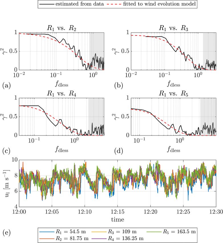
64 Y. Chen et al.: Parameterization of wind evolution using lidar
machine learning algorithm. The prediction process goes in Simley and Pao (2015) noted a limitation of this one-
the opposite direction: firstly, the wind evolution model pa- parameter model form: the intercept (coherence for 0 fre-
rameters are predicted by the trained parameterization mod- quency) of the modeled coherence is forced to be unity,
els using new predictor values calculated from new measured which is not always realistic. To overcome this issue, Sim-
data, and then, the predicted coherence is reconstructed by ley and Pao (2015) introduced a second parameter in the co-
the wind evolution model using the predicted model param- herence model, taking a model form similar to the coherence
eters. model for transverse and vertical separations suggested by
To demonstrate our concept and workflow: Sect. 2.3 ex- Thresher et al. (1981):
plains the wind evolution model used in this study; Sect. 2.4 s
2
discusses special issues regarding coherence estimation us- 2 fd
γmodel (f, d) = exp −a 0 + (b0 d)2 , (6)
ing lidar data; Sect. 2.5 discusses the potential predictors of U
the parameterization models; Sect. 2.6 and Sect. 2.7 briefly
introduce the principle of Gaussian process regression (the where a 0 and b0 are tuning parameters. A comparison be-
machine learning algorithm applied in this study) and the tween the fitting quality of a one-parameter model and a two-
method of model validation, respectively; Sect. 3.2 shows parameter model is given in Sect. 3.2 to confirm the necessity
the fitting process of the estimated coherence in detail; and of using a two-parameter wind evolution model.
Sect. 5 demonstrates the training of parameterization mod- We have made two modifications to Simley and Pao’s
els, predictor selection, and model validation in the respec- (2015) model. Firstly, d/U is restored to the travel time 1t to
tive subsections. avoid coupling the approximation of 1t = d/U in the wind
evolution model, considering the effect of the wind turbine’s
2.3 Wind evolution model induction zone. In fitting the estimated coherence to the wind
evolution model, 1t is determined by the time lag of the
Following the theoretical considerations by Ropelewski et al. peak of the cross-correlation between two wind speed sig-
(1973), the coherence decreases exponentially with increas- nals, indicated as 1tM . Secondly, a 0 b0 d is replaced with b.
ing evolution time 1t of the signal with respect to “eddy The reasons for that are the following. (1) With the original
turnover time” τ form a 0 b0 d, a 0 b0 is essentially the fitted term (given that d
is known) in the curve fitting. Thus, b0 shows a strong de-
2 1t
γmodel (f ) = exp −C · . (2) pendence on a 0 , which is generally undesirable for machine
τ
learning algorithms. (2) The form a 0 b0 d implies that this term
The term C represents the decay behavior of the coherence is proportional to d, but we found that d is still an important
depending on the time ratio. C could be a constant, a linear predictor for b0 , indicating that the assumption of a linear
function, or a more complicated term. τ is a timescale asso- relationship might be not proper. Therefore, we decided to
ciated with the characteristic eddy size λ and characteristic directly use b to represent the intercept and take d as a pre-
velocity of turbulence, which is approximated by the stan- dictor instead (see Sect. 2.5).
dard deviation of wind speed σ as follows: The modified wind evolution model is
q
λ 2
τ∼ . (3) γmodel (f ) = exp − a 2 · (f · 1t)2 + b2 , (7)
σ
This expression implies that eddies are supposed to decay where the decay parameter a represents the decay effect of
faster under strong turbulence. Given the same degree of tur- coherence and the offset parameter b is used to adjust the
bulence, large eddies are supposed to take a longer time to de- intercept (coherence for 0 frequency) of the modeled coher-
cay. The eddy size λ is linked to the frequency of horizontal- ence curve. The intercept equals exp(−|b|). Both parameters
wind-velocity fluctuations f and the flow mean wind speed are dimensionless. The term f · 1t is dimensionless and thus
U with the relation is defined as dimensionless frequency fdless . In the end, our
U wind evolution model is defined as
λ∼ . (4) q
f 2
γmodel 2
(fdless ) = exp − a 2 · fdless + b2 . (8)
Combining Eqs. (2)–(4), the coherence model becomes
In some studies (see, e.g., Schlipf et al., 2015), the wind
2
σ
γmodel (f ) = exp −C · · f · 1t . (5) evolution model is defined as a function of wavenumber k,
U with k = 2πf/U . The relationship between k and fdless is
This equation is essentially the same as the model proposed k = 2π fdless /d, applying the approximation of 1t = d/U .
by Pielke and Panofsky (1970), except that, in their model, To give an intuitive impression of the wind evolution model,
1t is approximated by d/U (d is separation) (Taylor, 1938; Fig. 2 shows the theoretical curves calculated with different
Willis and Deardorff, 1976), indicated as 1tT . values of a and b as examples.
Wind Energ. Sci., 6, 61–91, 2021 https://doi.org/10.5194/wes-6-61-2021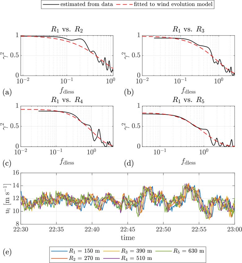
Y. Chen et al.: Parameterization of wind evolution using lidar                                                                         65

Figure 1. Concept and workflow of wind evolution prediction. The workflow of model training is the following. (1) Estimation of coherence
using lidar data. (2) Determination of wind evolution model parameters by fitting the estimated coherence to a wind evolution model.
(3) Calculation of potential predictors from measured data (mainly lidar data; sonic data could be involved if available). (4) Training of
parameterization models using a machine learning algorithm.

Figure 2. Impact of the model parameters a and b on the wind evolution model. (a) b = 0. (b) a = 3.

2.4   Estimating coherence using lidar data                            onto the laser beam and thus can be used to estimate the line-
                                                                       of-sight wind speed. The measurement principle of Doppler
In this work, the coherence is estimated with lidar data be-           wind lidar is explained in many publications (e.g., Weitkamp,
cause lidar can provide more data with respect to differ-              2005; Peña et al., 2013; Liu et al., 2019) and thus is not in-
ent spatial separations. This is not easy to obtain when us-           troduced here in detail.
ing meteorological towers because multiple towers would be                However, it must be emphasized that the coherence es-
needed, and only when the wind direction is aligned with the           timated with lidar data deviates from that estimated with
tower locations would the data be usable. Further, the predic-         data taken from ultrasonic anemometers. The reasons for
tion of the coherence is mainly expected to be applied when            that are the following. (1) The sampling rate of lidars is
coupled with the deployment of a lidar, e.g., in lidar-assisted        generally much lower than that of ultrasonic anemometers,
wind turbine control.                                                  and thus lidars cannot measure high-frequency fluctuations
   A Doppler wind lidar is a remote sensing device that mea-           in wind speed. (2) The measuring volume of lidars is gen-
sures wind speed based on the optical Doppler effect. Lidar            erally much longer than that of ultrasonic anemometers be-
emits laser pulses and detects the Doppler shift in backscat-          cause of its measurement principle, and thus for lidars, the
tered light from aerosol particles in the atmosphere that are          spatial-averaging effect within the measuring volume needs
entrained with the wind. The Doppler shift is proportional to          to be considered. (3) Lidars can only measure the wind speed
the line-of-sight wind speed, i.e., the wind speed projected

https://doi.org/10.5194/wes-6-61-2021                                                              Wind Energ. Sci., 6, 61–91, 2021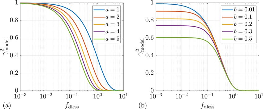
66                                                                   Y. Chen et al.: Parameterization of wind evolution using lidar

projected onto the emitted laser beams, i.e., the line-of-sight           Assume that the laser beam is aligned with the wind di-
wind speed. The influence of these three aspects is discussed          rection and Taylor’s (1938) hypothesis applies within the
in the following, specifically considering lidar in the staring        measurement volume and that Eq. (10) is also valid for the
mode.                                                                  Fourier transformation between the time and frequency do-
   Low sampling rate of lidar. According to the Nyquist–               mains. Taylor’s (1938) hypothesis is considered valid within
Shannon sampling theorem (Shannon, 1949), the upper fre-               the measurement volume because, in principle, wind evolu-
quency limit of a signal transformed from the time domain              tion depends on the evolution time of turbulence (see Eq. 2),
into the frequency domain is half of the sampling frequency.           and the measurement volume corresponds to a temporal
As long as the lidar sampling rate is sufficiently high to ac-         length on the order of magnitude of 10−7 s (typical length
quire a complete coherence curve covering the range from               of a laser pulse). Now, Eq. (11) can be written as (with t and
the highest coherence (e.g., 0.9–1.0) to the lowest coherence          f omitted for clarity)
(e.g., 0–0.1), it would probably not have a large impact on
studying the coherence. To obtain as high a sampling rate as             2                 |F{ui,l } · F ∗ {uj,l }|2
                                                                       γij,l =
possible, it is decided to select staring-mode data to calculate                 F{ui,l } · F ∗ {ui,l } · F{uj,l } · F ∗ {uj,l }
the coherence. Use of the staring mode generally means that                                        |F {w} · F {ui,p } · F ∗ {w} · F ∗ {uj,p }|2
the lidar measures the wind speed with a single laser beam                 =
                                                                               F {w} · F {ui,p } · F ∗ {w} · F ∗ {ui,p } · F {w} · F {uj,p } · F ∗ {w} · F ∗ {uj,p }
                                                                                                                                                                     .   (14)
pointing in a fixed direction. Specifically in this work, the
laser beam points horizontally upstream of the wind turbine.           Because the function w(x) is real and even, according to the
   Spatial-averaging effect of lidar. Consider a pulsed lidar          conjugate symmetry of the Fourier transformation (Oppen-
(only pulsed lidars are involved in this work). The spatial-           heim et al., 1997), F{w} = F ∗ {w} and F{w} is real and even
averaging effect can be modeled with a moving average                  as well. As a result, all instances of F{w} in the denomina-
weighted by a Gaussian-like shape function (see, e.g., Cari-           tor and the numerator are canceled out. And thus Eq. (14)
ous, 2013) or a triangular function (see, e.g., Sathe and Mann,        becomes:
2012) centered at a measurement point. Following Carious                                   |F{ui,p } · F ∗ {uj,p }|2
                                                                         2                                                           2
(2013), the weighting function w(x) is an even function cen-           γij,l =                                                   = γij,p .                               (15)
                                                                                 F{ui,p } · F ∗ {ui,p } · F{uj,p } · F ∗ {uj,p }
tered at every measurement point along the laser beam. The
lidar-measured wind speed at the measurement point x0 for              This means that the spatial-averaging effect does not influ-
any instant can be modeled with                                        ence the coherence under the above-mentioned ideal assump-
             Z∞                                                        tions.
ul (x0 ) =        w(x0 − x)up (x)dx = (w ∗ up )(x0 ),         (9)         Misalignment of wind direction and lidar measurement.
                                                                       The above derivation is based on an important assumption
          −∞
                                                                       that the laser beam is aligned with the wind direction. This
where up (x) is a wind speed function of spatial points on the         will not always be fulfilled in reality, even for a nacelle-
x axis aligned with the lidar’s laser beam. According to the           mounted lidar operating in the staring mode. Figure 3 shows
convolution theorem (Oppenheim et al., 1997), the following            a misalignment between wind direction and lidar measure-
relationship is valid for the Fourier transformation between           ment direction, at an angle α. The coherence of the line-of-
space and the wavenumber domain                                        sight wind speed is γ122 , which is no longer the longitudinal

F{ul } = F{w ∗ up } = F{w} · F{up },                         (10)      coherence but the horizontal coherence as defined by Panof-
                                                                       sky and Mizuno (1975). γ13  2 and γ 2 are the longitudinal and
                                                                                                           23
where F{ } is the Fourier transform operator.                          lateral coherence, respectively.
  Following Eq. (1), the coherence estimated with lidar data,             Schlipf et al. (2015) suggested a model for the horizontal
indicated with the subscript “l’’, is                                  coherence (magnitude coherence) based on the assumption
                                                                       of point measurement for simplification
  2                |Sij,l (f )|2
γij,l (f ) =                           ,                     (11)
               Sii,l (f ) · Sjj,l (f )                                                    cos2 (α)γij,ux γij,uy Sii,u
                                                                       γij,losP =                                                       ,                                (16)
where Sii,l (f ) and Sjj,l (f ) are the auto-spectrum at the point                    cos2 (α)Sii,u + sin2 (α)Sii,v
i and j , respectively; Sij,l (f ) is the cross-spectrum between
i and j ; and f is the frequency in Hz. They are all estimated         where γij,losP is the horizontal coherence of line-of-sight
from lidar data. The auto-spectrum is                                  wind speed point measurements, γij,ux and γij,uy are the lon-
                                                                       gitudinal and lateral coherence of the longitudinal wind com-
Sii,l (f ) = F{ui,l (t)} · F ∗ {ui,l (t)},                   (12)      ponent, and Sii,u and Sii,v are the auto-spectra of the longi-
                                                                       tudinal and lateral wind components. Based on this equation,
where ui,l (t) is the time series of the wind speed at i, and the
                                                                       determining the longitudinal coherence γij,ux is possible only
symbol ∗ means conjugate. And the cross-spectrum is
                                                                       given a specific turbulence model (knowing Sii,u , Sii,v , and
Sij,l (f ) = F{ui,l (t)} · F ∗ {uj,l (t)}.                   (13)      γij,uy ) and knowing the misalignment angle α. Moreover, the

Wind Energ. Sci., 6, 61–91, 2021                                                                          https://doi.org/10.5194/wes-6-61-2021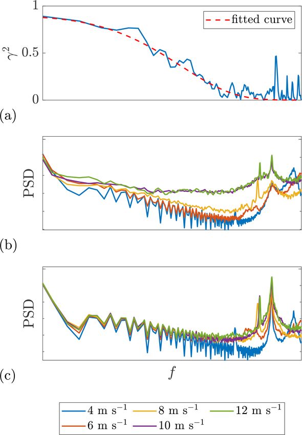
Y. Chen et al.: Parameterization of wind evolution using lidar                                                                       67

                                                                        regression inherently assumes imperfect training data (con-
                                                                        taining noisy terms; see Sect. 2.6), so it is better to keep un-
                                                                        certainties in predictors.
                                                                           Certainly, if the direction misalignment is available and
                                                                        sufficiently accurate in a given application scenario, the pre-
                                                                        diction concept can be easily adjusted by changing the wind
                                                                        evolution model to which the estimated coherence is sup-
                                                                        posed to fit.

                                                                        2.5   Potential predictors
                                                                        In the literature reviewed in the Introduction, the variables
                                                                        considered relevant to wind evolution are as listed below:
Figure 3. Misalignment of wind direction and lidar measurement.
                              2 is the coherence of the line-of-sight
α is the misalignment angle. γ12                                          – Ropelewski et al. (1973): turbulence intensity (a func-
               2       2
wind speed. γ13 and γ23 are the longitudinal and lateral coherence,         tion of roughness length and the Richardson number;
respectively.                                                               Lumley and Panofsky, 1964);
                                                                          – Panofsky and Mizuno (1975): mean wind speed, turbu-
                                                                            lence intensity, standard deviation of the lateral wind
above-discussed spatial-averaging effect must be coupled to                 component, lateral integral length scale of the longitu-
the horizontal coherence, considering that the lateral coher-               dinal wind component, longitudinal separation, and the
ence for the point at x depends on the lateral separation 1y                angle between the wind direction and the measurement
associated with its distance from the center point of the range             line (if misalignment exists);
gate x0 , i.e., 1y = cos(α)(|x − x0 |). Therefore, the longitudi-
nal coherence is implicitly included in the integration of hor-           – Kristensen (1979): turbulence intensity, longitudinal in-
izontal coherence weighted by the range-weighting function                  tegral length scale of the longitudinal wind component,
of lidars.                                                                  and longitudinal separation;
   In this study, we decide to develop a parameterization
                                                                          – Simley and Pao (2015): turbulence intensity, longitudi-
model based on horizontal coherence for the following rea-
                                                                            nal integral length scale of the longitudinal wind com-
sons. Firstly, consider the case for a nacelle-mounted lidar.
                                                                            ponent, and longitudinal separation.
The misalignment of the lidar measurement means that the
wind turbine is misaligned as well. In this case, it makes                 The above-mentioned variables can be categorized into
sense to predict the corresponding horizontal coherence. Sec-           three groups: wind statistics, atmospheric stability, and rela-
ondly, a standalone parameterization model, independent of              tive positions of measurement points. We follow this train of
any turbulence model, is desired for more flexibility in ap-            thought to discuss potential predictors of the parameteriza-
plication. Thirdly, determining the parameters in an implicit           tion models. It is worth mentioning, in advance, that not all
wind evolution model is complicated when using measured                 of these predictors will be used in the final models. Useful
data. And it is necessary to acquire the misalignment angle α,          features will be selected using the automatic relevance de-
which is not always possible in application, especially when            termination squared exponential kernel function (Duvenaud,
lidar is the only data source, though deployment of lidars              2014). The goal of this initial step is to collect all possible
with multiple beams might help in this case. Moreover, the              predictors, even though some of them will turn out to be re-
requirement for the accuracy of α is very high because α is             dundant and can be converted to each other.
included in the most basic step – fitting the estimated co-                Wind statistics. Following prior research, turbulence inten-
herence to the wind evolution model. The uncertainties con-             sity IT is considered as a predictor. The turbulence intensity
tained in α will propagate through the whole model and af-              is defined as
fect the further analysis radically. Since the prediction con-                 σ
cept needs to be applicable under different data availabilities,        IT = .                                                     (17)
                                                                              U
it is not desired to make the fitting process depend so crit-
ically on a variable whose availability and accuracy are not            In addition, mean wind speed U and its standard deviation σ
always guaranteed. It is thus helpful to consider α as a predic-        are also included because they are the fundamental variables
tor (see Sect. 2.5) to account for variations in the horizontal         of turbulence intensity. Apparently, IT and σ are equivalent
coherence caused by the direction misalignment. The benefit             (given U ), so only one of them will be selected according to
of doing so is to make α more standalone and to prevent its             the result of feature selection.
errors from affecting everything else, while reasonably tak-               Moreover, integral length scale L is considered as a pre-
ing its influences into account. In addition, Gaussian process          dictor and approximated with (Pope, 2000; Simley and Pao,

https://doi.org/10.5194/wes-6-61-2021                                                              Wind Energ. Sci., 6, 61–91, 2021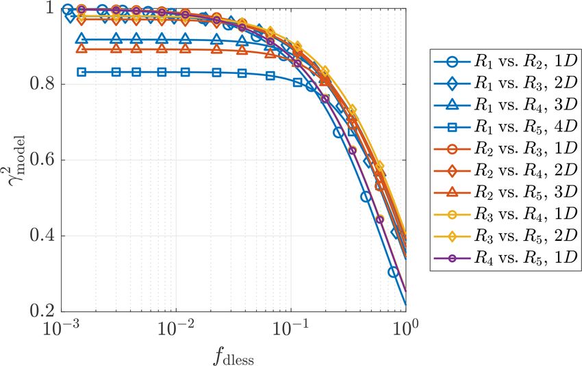
68 Y. Chen et al.: Parameterization of wind evolution using lidar
2015) a simple level, whether these two high-order wind statistics
could be useful for prediction.
Z∞ Atmospheric stability. The atmospheric stability represents
L = U · ρ(s)ds = U · T , (18) a global effect of the surface layer in the boundary layer on
0 a wind field. It is believed to affect wind evolution, being
an influence factor on turbulence stability (Ropelewski et al.,
where ρ(s) is the autocorrelation function. Indeed, integrat- 1973; Lumley and Panofsky, 1964). A dimensionless height
ing the autocorrelation gives the integral timescale T . The ζ , built with Obukhov length LMO (Obukhov, 1971), is con-
approximation of L is essentially based on assuming the tur- sidered as a predictor (Businger et al., 1971)
bulent eddies advected by the mean flow at U . Please note
that this is not necessarily equivalent to assuming “frozen” z κgw0 θv0 z
turbulence. Turbulent eddies can evolve when preserving the ζ= =− , (21)
LMO θ u3∗
same mean wind speed and statistical properties (including
autocorrelation). The multiplication of U can be understood where κ is the von Kármán constant, g is gravitational accel-
as translating the integration domain from time lag s to spa- eration, z is the measurement height, θ is the mean potential
tial separation by approximating the spatial separation with temperature, u∗ is the friction velocity, and w0 θv0 is the co-
U ·s. This approximation might contain uncertainties, but we variance of vertical velocity perturbations and virtual poten-
have no alternatives for calculation of L from measured data. tial temperature.
The integration of autocorrelation is computed up to the first Relative positions of measurement points. Based on
zero-crossing location instead of infinity in practice (Simley our modifications to Simley and Pao’s (2015) model (see
and Pao, 2015). Considering the correlation between L and Sect. 2.3), measurement separation d has been removed from
T shown in Eq. (18), T is also considered as a predictor, and the wind evolution model and is now considered as a predic-
thus L and T constitute another pair of redundant predictors tor. As discussed in Sect. 2.4, the misalignment angle α is not
from which only one will be selected. involved in fitting the wind evolution model but is considered
Besides the variables already considered in prior studies, as a predictor to account for the influence of the lateral co-
it is interesting to explore whether high-order wind statistics herence on the horizontal coherence. In fact, d is associated
such as skewness and kurtosis of wind speed could play a with two different effects. On the one hand, d corresponds to
role in wind evolution prediction. Skewness (i.e., the third travel time or, rather, to evolution time 1t, which is believed
standardized central moment) and kurtosis (i.e., the fourth to play an important role in wind evolution. On the other
standardized central moment) are measures of the asymme- hand, d together with α account for the decay of the lateral
try and flatness of the wind speed distribution, respectively. coherence. The travel time determined with the maximum
The sample skewness G1 , with bias correction, is defined as cross-correlation 1tM is a more accurate variable. However,
(Joanes and Gill, 1998) considering that calculating 1tM might not always be feasi-
√ 1 Pn
ble due to its computational complexity, the travel time ap-
n(n − 1) u3 proximated using Taylor’s (1938) translation hypothesis 1tT
G1 = · n i=1 i 3/2 , (19)
n−2 1 Pn 2 is included as well.
n i=1 ui
The notations of the above-mentioned potential predictors
are summarized in Table 1. These variables are derived from
and the sample kurtosis G2 (not subtracting 3), with bias cor-
both lidar data and data measured with ultrasonic anemome-
rection, is defined as (Joanes and Gill, 1998)
ters (hereafter referred to as sonic data) according to their
n−1 availability in each measurement campaign. The measure-
G2 = ment instrument is indicated with a subscript: “l” for lidar
(n − 2)(n − 3)
and “s” for sonic (i.e., ultrasonic anemometer). For exam-
1 Pn 4 ple, Ul represents the mean wind speed calculated from lidar
u
· (n + 1) · n i=1 i2 − 3(n − 1) + 3, (20)
data. Regarding sonic data, it is more reasonable for the anal-
1 P n 2
n i=1 ui ysis of wind evolution to use a wind coordinate system with
the x axis aligned to the mean wind direction instead of the
where ui is wind speed fluctuations and n is the number of meteorological coordinate system. The mean wind direction
data points. According to Lenschow et al. (1994), statistical is determined with the mean wind direction for each data
moments estimated using time series data with limited length block. The high-resolution longitudinal (indicated with the
show a systematic deviation from the true moments and also subscript “x”) and lateral (indicated with the subscript “y”)
contain random errors. Both are decreasing functions of the wind speeds are obtained by projecting the high-resolution
averaging time. Compared to the sample standard deviation, wind components measured with ultrasonic anemometers on
the sample skewness and kurtosis would probably contain the wind coordinate system. Then, the above-mentioned vari-
larger uncertainties. Nevertheless, we still want to test, on ables are derived from the data based on the wind coordinate
Wind Energ. Sci., 6, 61–91, 2021 https://doi.org/10.5194/wes-6-61-2021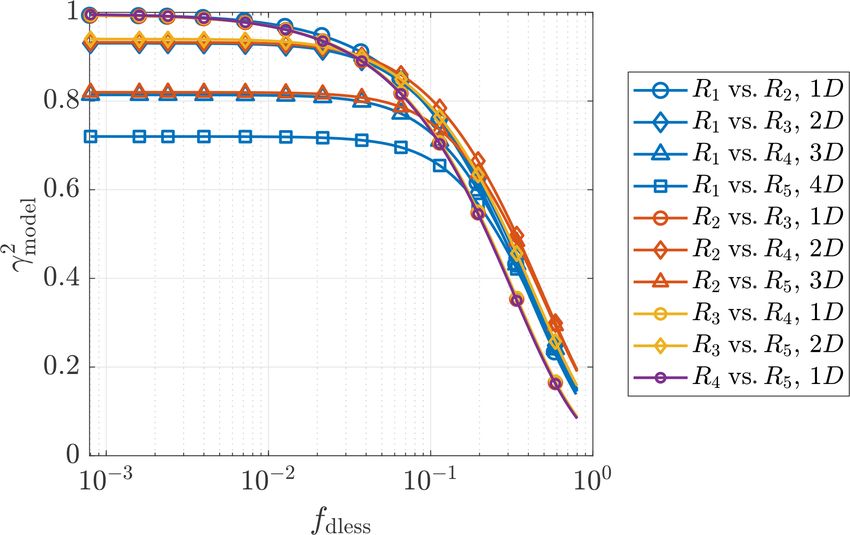
Y. Chen et al.: Parameterization of wind evolution using lidar                                                                        69

system. For example, Ux,s represents the mean wind speed               tributed Gaussian noise with zero mean and variance σn2
calculated from the longitudinal wind component measured
with ultrasonic anemometers.                                           ε ∼ N (0, σn2 ).                                             (23)

                                                                       The Bayesian linear model is a GP given that the prior distri-
2.6   Gaussian process regression                                      bution of w is normally distributed with zero mean. Since
                                                                       a GP is fully specified by its mean and covariance, the
This section briefly introduces the principle of the Gaussian          Bayesian linear model is written as
process regression (GPR) and the hyperparameters that mod-
ify the behavior of a GPR model. The model training is done            f (X) ∼ GP(0, cov(f (X))),                                   (24)
using the MATLAB Statistics and Machine Learning Tool-
box1 .                                                                 where X is the aggregation of all input vectors of n observa-
   The principle of GPR. Consider making a regression                  tions. This is the prior distribution over functions. The pres-
model from some data. A very intuitive approach is to fit              ence of ε shows another advantage of GPR, viz. that it is able
certain functions, e.g., linear or polynominal. However, this          to inherently assume noisy observations and take this effect
requires an initial guess about the functional relationship(s)         into account in the model. σn is one of the hyperparameters.
behind the data, which is very difficult in this case because             It is common, but not necessary, to assume GPs with a zero
the wind evolution model parameters do not indicate any                mean function. The mean function can be modeled with a set
clear dependence on the potential predictors. The reasons              of basis functions h(x) and a corresponding coefficient vec-
for that could be multiple: (1) the data could be noisy; and           tor β. So, GPs with a non-zero mean function can be assumed
(2) the dependence could exist in multidimensional space               as
not observable in a single dimension, etc. Under this cir-
cumstance, GPR turns out to be a good choice because it is             g(x) = f (x) + h(x)> β.                                      (25)
non-parametric probabilistic model, which means the model              The basis function is one of the hyperparameters. MATLAB
is not a specific function, but a probability distribution over        provides four types of basis function: zero (assuming no ba-
functions. The principle underlying GPR is Bayesian infer-             sis function), constant, linear, and pure quadratic. The coeffi-
ence. The prior distribution over functions, which can be un-          cient vector β can also be understood as the weight vector of
derstood as a guess about what kinds of function could be              h(x). But we have defined w as a weight vector in Eq. (22),
present without knowing the data, is specified by a particular         we want to avoid using the same word here in case reader
Gaussian process (GP) which favors smooth functions. In the            might confuse these two different processes. β is estimated
training process, as adding the data, the probabilities associ-        from training data.
ated with the functions which do not agree with the observa-              The covariance of the function values is not specified ex-
tions will be decreased, which gives the posterior distribution        plicitly but estimated using a kernel function
over the functions (Rasmussen and Williams, 2006).
   Hyperparameters of GPR. The behavior of a GPR model                 cov(f (X)) = K(X, X),                                        (26)
is defined by its hyperparameters. To introduce the hyperpa-
rameters, a basic explanation is given following Rasmussen             which is the so-called kernel trick. There are two types of
and Williams (2006). Please note that the complete deduction           kernel functions: one is kernel functions with the same char-
is not displayed here because it is beyond the scope of this pa-       acteristic length scale for all predictors; the other has separate
per. For further details, please refer to chap. 2 of Rasmussen         characteristic length scales. The latter are called automatic
and Williams’ (Rasmussen and Williams, 2006) book.                     relevance determination kernel functions and can be used to
   GPR is based on Bayesian inference. First, consider a sin-          select predictors. The kernel function and its characteristic
gle observation. The Bayesian linear regression model with             length scale(s) are hyperparameters of the GPR model.
Gaussian noise is defined as                                              In this work, automatic relevance determination squared
                                                                       exponential kernel function (ARD-SE kernel) (Duvenaud,
f (x) = φ(x)> w,      y = f (x) + ε,                           (22)    2014) is applied. The ARD-SE kernel function is basically a
                                                                       squared exponential kernel function (SE kernel) with a sep-
where x is an input vector containing D different predic-              arate characteristic length scale σm for each predictor m (m
tors of a single observation, φ(x) is the function which maps          is the index of predictors). For any pairs of observations i, j ,
the input vector onto a higher dimensional space where the             the ARD-SE kernel function is defined as
Bayesian linear model is applicable, w is a vector of weights                                "
                                                                                                    D
                                                                                                                       #
of the linear model, f (x) is the function value, y is the                              2        1X     (xim − xj m )2
                                                                       K(x i , x j ) = σf exp −                          ,           (27)
observed target value, and ε is independent identically dis-                                     2 m=1       σm2

   1 https://de.mathworks.com/products/statistics.html, last access:   where σf2 denotes the signal variance, which determines the
18 June 2020                                                           variation of function values from their mean. In the context of

https://doi.org/10.5194/wes-6-61-2021                                                             Wind Energ. Sci., 6, 61–91, 2021
70                                                                  Y. Chen et al.: Parameterization of wind evolution using lidar

Table 1. Notations of potential predictors.

                             Notation    Variable                                                  Unit
                             U           Mean wind speed                                           [m s−1 ]
                             σ           Standard deviation of wind speed                          [m s−1 ]
                             G1          Skewness of wind speed                                    [–]
                             G2          Kurtosis of wind speed                                    [–]
                             IT          Turbulence intensity                                      [–]
                             T           Integral timescale                                        [s]
                             L           Integral length scale                                     [m]
                             ζ           Dimensionless Obukhov length                              [–]
                             d           Measurement separation                                    [m]
                             α           Angle between wind direction and lidar measurement        [◦ ]
                             1tM         Travel time determined by the maximum cross-correlation   [s]
                             1tT         Travel time approximated by d/U                           [s]

machine learning, the characteristic length scale σm is not a         training data ( k−1
                                                                                       k of the total observations) could be insuffi-
“length” in the physical sense; it is a characteristic magnitude      ciently large. However, considering that the training process
for the predictor m which implies the sensitivity of the func-        must be repeated k times, it would take a very long time when
tion being modeled to the predictor m. A relatively large σm          k is very large. As a compromise between these two factors,
indicates a relatively small variation along the corresponding        k is commonly set to 5–10 in machine learning. In this study,
dimensions in the function, which means these predictors are          5-fold cross-validation is applied.
less relevant than the others (Duvenaud, 2014).                          The model performance is evaluated with two goodness-
   In the end, the key predictive equation for GPR can be             of-fit measures: root mean square error (RMSE),
derived by conditioning the joint Gaussian prior distribution                    v
on the observations, and it is normally distributed.                             u
                                                                                 u1 X   N
                                                                      RMSE = t            (yi − ypred,i )2 ,                    (29)
f ∗ |X, y, X∗ ∼ N (f ∗ , cov(f ∗ )),                         (28)                   N i

where X∗ denotes new input data used in the prediction. f ∗           and the coefficient of determination (R 2 ),
represents f ( X∗ ) for convenience, which is the predicted
function value.                                                                 PN
                                                                                     (yi − ypred,i )2
   To summarize, the hyperparameters defining a GPR model             R = 1 − iP
                                                                        2
                                                                                                2
                                                                                                      ,                         (30)
                                                                                      i (yi − y)
are the basis function h(x), the noise standard deviation
of the Gaussian process model σn , the kernel function                where y and ypred denote the observed and predicted target
K(x i , x j ), the standard deviation of the function values σf ,     values, respectively; y denotes the average of the observed
and the characteristic length scale in the kernel function σm .       target values; and N denotes the number of observations. It
These hyperparameters can be tuned in the training process            is worth mentioning that, according to this definition, R 2 can
to achieve a better model.                                            be understood as taking the prediction with the mean value
                                                                      of the observations as a reference by which to evaluate the
2.7   Model validation                                                model performance. In this case, R 2 ranges from −∞ to
                                                                      one, for perfect prediction. R 2 equals zero if the prediction
The trained model is evaluated with a k-fold cross-validation         is made simply with the mean value of the observations. The
in which the data are divided into k disjoint, equally sized          higher R 2 is, the better the model performs. A negative value
subsets. The model validation is done with one subset (also           of R 2 indicates that the selected model performs even worse
called in-fold observations), and the training is done with the       than prediction using just the mean value of the observations.
remaining (k − 1) subsets (also called out-of-fold observa-
tions). This procedure is repeated k times, each time with
a different subset for validation. The predicted target values        3   Data processing
and the goodness-of-fit measures of the regression models
                                                                      This section first introduces the data sources in Sect. 3.1 and
are computed for in-fold observations using a model trained
                                                                      then explains the procedure for the determination of the wind
on out-of-fold observations.
                                                                      evolution model parameters in Sect. 3.2.
   Theoretically, k can be any integer between 2 and the num-
ber of observations (a special case called “leave-one-out”
cross-validation). When k is very small, the sample size of

Wind Energ. Sci., 6, 61–91, 2021                                                           https://doi.org/10.5194/wes-6-61-2021
Y. Chen et al.: Parameterization of wind evolution using lidar 71
3.1 Data source Compared to ultrasonic anemometers, lidar systems have
much lower sampling rates. To obtain the highest possible
This study involves measured data from two research sampling rate, we select the measurement periods where the
projects. The reasons for using two different data sources are, staring mode was used, for both campaigns.
on the one hand, to find commonality between two different Essential information about the measurements is summa-
measurements and avoid accidental conclusions and, on the rized in Table 2. Figure A1 gives an overview of the wind
other hand, to study whether there are differences or what statistics of these two selected measurement periods by illus-
kind of differences in the wind evolution can be observed. trating the relative-frequency distribution of lidar-measured
The relevant research projects as well as the measurement wind speed and turbulence intensity. For brevity, “Lidar
campaigns are (briefly) as follows. Complex” and “ParkCast” are used to refer to the selected
Lidar Complex. The research project Lidar Complex was measurements throughout the paper.
funded by the German Federal Ministry for Economic Af-
fairs and Energy (BMWi). In this project, a lidar measure-
ment campaign was carried out in Grevesmühlen, Germany. 3.2 Determination of wind evolution model parameters
The measurement site is basically flat, mainly farmland with To obtain the wind evolution model parameters a and b, the
hedges and a few large trees. More details about the measure- wind evolution is estimated with lidar data and then fitted to
ment campaign can be found in Schlipf et al. (2015). The li- the wind evolution model (Eq. 8). The processing procedure
dar deployed in this measurement campaign was the SWE is described as follows.
(Stuttgart Wind Energy) Scanner 1.0, which was adapted Step 1: filtering of the lidar data. The lidar data from Lidar
from a WindCube V1 from Leosphere (Schlipf et al., 2015). Complex are filtered according to the carrier-to-noise ratio
This lidar has five measurement range gates focusing at dis- (CNR) of the lidar signals (CNR filter). The valid range of
tances of 54.5, 81.75, 109, 136.25, and 163.5 m, respectively. the CNR filter is −24 to −5 dB, determined from the plot of
The full width at half maximum (FWHM) of the measure- CNR values and wind speed.
ment range gates is 30 m (Carious, 2013). The lidar was in- A CNR filter is not, however, suitable for lidar data from
stalled on the nacelle of a wind turbine (rotor diameter of ParkCast because, for a long-range lidar, the backscattered
109 m) at 95 m. In addition, a meteorological mast is located signals from distant range gates could be very weak, and
295 m southwest of the wind turbine; data from an ultrasonic thus the CNR values could be low even when the measured
anemometer installed at 93 m on the meteorological mast are wind speed is plausible. Würth et al. (2018) suggested an
also involved in this study. SCADA (supervisory control and approach to filter the data based on the value range (range
data acquisition) data of the wind turbine are also available. filter) and the standard deviation (standard-deviation filter)
Recorded yaw positions are used to estimate the misalign- within a certain number of adjacent data points defined as a
ment angle α, assuming that the mean wind direction at the window, which can keep more valid data than a CNR filter.
turbine can be approximated with the mean wind direction A range filter detects the maximum value difference within
measured on the meteorological mast. a window and filters the data points for which the maximum
ParkCast. The ParkCast2 project is an ongoing project value difference exceeds a threshold. A standard-deviation
funded by the German Federal Ministry for Economic Af- filter calculates the standard deviation within a window and
fairs and Energy (BMWi). While this paper is in prepara- filters the data points for which the standard deviation ex-
tion, a lidar measurement campaign is being conducted on ceeds a threshold. Both filters are applied to check the line-
the offshore wind farm “alpha ventus”3 . Two long-range li- of-sight wind speed with thresholds of 6 m s−1 and 3 m s−1 ,
dars (StreamlineXR) have been deployed in the measurement respectively. The window size is set to three data points.
campaign. The data used here are from the lidar installed on Step 2: estimation of coherence. The lidar data are di-
the nacelle of wind turbine AV4 (rotor diameter of 126 m) at vided into 30 min blocks. This is consistent with the com-
92 m, measuring the inflow. The measurement distances were monly used period for calculating the Obukhov length. Only
set to 30–990 m with an increment of 60 m. The FWHM of the data blocks with more than 80 % valid data points are
the measurement range gates is 60 m. Unfortunately, neither used to estimate the coherence. The missing values are es-
data from the meteorological mast on FINO14 nor SCADA timated by shape-preserving piecewise cubic interpolation
data of AV4 for the observed period were available when the (Fritsch and Carlson, 1980). The missing end values are each
analysis was done. Therefore, the misalignment angle α is replaced with their nearest value. Data measured at differ-
not available for ParkCast. ent range gates (i.e., measurement distances) are paired in
2 https://www.rave-offshore.de/en/parkcast.html, last access: the way shown in Fig. 4 to obtain as many samples (i.e.,
18 June 2020 data blocks) as possible. The pairing has N2 possibilities
3 https://www.alpha-ventus.de/english, last access: 18 June 2020 (N is the number of the lidar range gates). The travel time
4 Forschungsplattform In Nord- und Ostsee Nr. 1 (Research Plat- of the wind field is approximated with the time lag at the
form in the North and Baltic Seas No. 1); https://www.fino1.de/en/, maximum of the cross-correlation 1tM between these two
last access: 18 June 2020 wind speed signals. The upstream point is always regarded
https://doi.org/10.5194/wes-6-61-2021 Wind Energ. Sci., 6, 61–91, 202172 Y. Chen et al.: Parameterization of wind evolution using lidar
Table 2. Summary of measurement setups.
Measurement campaign Lidar Complex ParkCast
Selected period 2 to 20 Dec 2013 4 to 14 Jun 2019
Location Grevesmühlen, Germany alpha ventus
Terrain type Onshore, flat Offshore
Device Nacelle-based lidar and met mast Nacelle-based lidar
Measurement height [m] 95 (lidar), 93 (sonic) 92
Range gate [m] 54.5, 81.75, . . ., 163.5 30, 90, . . ., 990
Number of range gates 5 17
Full width at half maximum [m] 30 60
Sampling rate [Hz] 0.99 0.27
Valid samples∗ 3285 10112
∗ After lidar data filtering, data pairing, and outlier filtering. For details see Sect. 3.2.
quency fdless is fdless = kd/2π . Thus, the smallest critical
value of fdless is d/WL . Considering Lidar Complex as an
example, WL = 30 m and d = 27.25 m for the smallest sepa-
ration, which is the most critical case. d/WL ≈ 0.91, which
is already located in the filtered part (see the grey area in
Fig. 5a).
The fitting is done by a nonlinear least-squares method us-
Figure 4. Pairing of different range gates for estimating coherence
ing the Levenberg–Marquardt algorithm (Levenberg, 1944;
for Lidar Complex, given as an example.
Marquardt, 1963; Moré, 1978). Only the data blocks with
R 2 > 0.8 are considered as valid samples.
Step 4: outlier filtering. The final filtering was done by
as the reference point. The data measured at the downstream checking the value distribution of every relevant variable to
point are shifted by 1tM to match the reference wind speed omit outliers. It is emphasized that outliers are not necessar-
data. The magnitude-squared coherence is estimated using ily false data. In some cases, the outlier is from a value range
Welch’s overlapped averaged periodogram method using a in which not enough samples were collected. It is very im-
Hamming window, 24 segments, and 50 % overlap. The data portant to filter outliers properly because it is difficult for a
of the reference point are used to calculate lidar-measured regression model to capture the relationship for those value
wind statistics. ranges with too few samples. Because the distributions of the
Step 3: fitting to the wind evolution model. Before fitting variables all have a long right tail, the outliers are chosen as
the model, we must consider two issues that might introduce all data exceeding the 99th percentile of the data.
noise into the coherence estimate. Firstly, because both lidars Figure 5 is an example plot of the data block from 7 De-
are installed on the nacelle of a wind turbine which is actu- cember 2013 at 12:00–12:30 from Lidar Complex. This
ally in motion; the focus points of the laser beams are moving data block is selected here for two reasons: data integrity
as well. This motion causes excitation at certain frequencies and representative wind statistics. In this data block, the
in the estimated coherence. Figure A2 shows a comparison lidar-measured mean wind speed is 7.3–7.7 m s−1 , and the
between an example coherence curve and the power spectral lidar-measured turbulence intensity is 0.10–0.12, for differ-
density (PSD) of the fore-aft and in-plane tower top acceler- ent range gates. These values appeared frequently in the se-
ation of Lidar Complex. The excitation in the coherence con- lected period according to Fig. A1. Hence, this data block
forms to that in both PSDs and occurs mainly at frequencies is regarded as a representative case-study example for Lidar
above 0.2 Hz. To avoid negative effects on the fitting quality Complex and is referred to throughout the paper. The figure
caused by this excitation, the cutoff frequency is hence set illustrates the estimated coherence between different range
at 0.2 Hz, and the coherence is fitted only up to this cutoff gates and the corresponding fitted curves. The shaded areas
frequency. show that the selected cutoff frequency of 0.2 Hz is reason-
Secondly, according to Schlipf (2015), critical wavenum- able for this case. A similar plot from ParkCast is found in
bers where the lidar signals would be only determined Fig. A3. Because the sampling rate of ParkCast is lower, the
by noises must be checked. The critical wavenumbers are excitation by the nacelle’s movement is not observed in the
2π/WL (WL is the full width at half maximum of the range coherence, and thus no cutoff frequency was set for ParkCast
gate) and its harmonics. As mentioned in Sect. 2.3, the re- data.
lationship between wavenumber k and dimensionless fre-
Wind Energ. Sci., 6, 61–91, 2021 https://doi.org/10.5194/wes-6-61-2021You can also read