Modelling Gravel Beach Profile Evolution Using Parametric and Process-Based Models

UNIVERSITY OF SOUTHAMPTON

Modelling Gravel Beach Profile Evolution
 Using Parametric and Process-Based
 Models

 Name: Jake Carley
 Student ID: 31476058
 Academic Supervisor: Dr Hachem Kassem

 MSc Engineering in the Coastal Environment
 Faculty of Engineering in the Environment and the
 School of Ocean and Earth Sciences

 Main Body Word Count: 18908

 September 2020

Declaration
This thesis was submitted for examination in September 2020. It does not necessarily represent
the final form of the thesis as deposited in the University after examination.

I, Jake Carley declare that this thesis and the work presented in it are my own and has been
generated by me as the result of my own original research.

I confirm that:
1. This work was done wholly or mainly while in candidature for a degree at this University;

2. Where any part of this thesis has previously been submitted for any other qualification at
this University or any other institution, this has been clearly stated;

3. Where I have consulted the published work of others, this is always clearly attributed; 4.
Where I have quoted from the work of others, the source is always given. With the exception
of such quotations, this thesis is entirely my own work;

5. I have acknowledged all main sources of help;

6. Where the thesis is based on work done by myself jointly with others, I have made clear
exactly what was done by others and what I have contributed myself;

7. Either none of this work has been published before submission, or parts of this work have
been published as: [please list references below]:

 i

Abstract
Understanding and predicting sediment transport processes on gravel beaches is becoming
increasingly important for engineers and coastal protection schemes, as the increased
frequency and severity of storm events threatens the vast infrastructure situated along many
areas of the UK coastline. Gravel beaches are growing in popularity as a natural form of
coastal defence due to their ability to dissipate wave energy; yet, the predictive methods of
the morphodynamic response to storms are less well established than sandy beach
environments. Here this study assesses the suitability of two existing gravel beach models,
process-based (XBeach-G) and parametric (Shingle-B); for predicting shoreline evolution on
the mixed sand-gravel barrier at Pevensey. Simulated output profiles validated for two
extreme storm events (13/12/2011 and 15/2/2014), indicate that quantitively both models are
able to predict the response of the entire morphological profile reasonably well. Beside this,
wave run-up elevations predicted by both models are comparable to values estimated by the
EurOtop 2007 formula (max variance

Acknowledgements
I would like to give a special thank you to my academic supervisor Dr Hachem Kassem, for
the continued support you provided throughout this research project and your passion for
coastal processes in general. Despite working remotely for this project, you would always
find time to schedule a meeting and provide constructive feedback on my work. I would also
like to thank Dominique Townsend for sharing her knowledge of GIS and providing guidance
on beach nourishment at Pevensey for my data analysis. I am also extremely privilidged and
grateful to Dr Sam Cope and the Standing Conference on Problems Associated with the
Coastline (SCOPAC), for presenting me with this year’s Andy Bradbury Bursary for the
research project scoping study. A final thank you goes to the Channel Coastal Observatory
(CCO), for providing the wave and topographic data for validation in the study.

 iii

Contents

Acknowledgements............................................................................................................. iii

List of Figures..................................................................................................................... vi

List of Tables ...................................................................................................................... ix

Glossary ............................................................................................................................... x

Chapter 1: Introduction ...................................................................................................... 1

 1.1 Background ................................................................................................................. 1

 1.2 Aims and Objectives .................................................................................................... 2

Chapter 2: Literature Review ............................................................................................. 4

 2.1 Gravel Beach Origins................................................................................................... 4

 2.2 Gravel Beach Morphodynamics ................................................................................... 4

 2.3 Hydraulic Conductivity and Groundwater Exchange .................................................... 6

 2.4 Measuring Sediment Transport on Gravel Beaches ...................................................... 8

 2.5 Storm Impacts on Gravel Beaches ................................................................................ 9

 2.6 Modelling Gravel Beaches ......................................................................................... 10

Chapter 3: Methodology ................................................................................................... 12

 3.1 Study Site .................................................................................................................. 12

 3.1.1 Overview......................................................................................................................... 12
 3.1.2 Current Beach Management ........................................................................................... 14
 3.1.3 Management Profiles ...................................................................................................... 14
 3.2 Previous Research at Pevensey Bay ........................................................................... 15

 3.3 Data Observations...................................................................................................... 16

 3.3.1 2011 Storm Event............................................................................................................ 17
 3.3.2 2014 Storm Event............................................................................................................ 18
Chapter 4: Model Overview and Setup ............................................................................ 21

 4.1 Model Description ..................................................................................................... 21

 4.1.1 XBeach-G ........................................................................................................................ 21
 4.1.2 Shingle-B ......................................................................................................................... 22

 iv

4.2 Model Setup .............................................................................................................. 23

 4.2.1 XBeach-G ........................................................................................................................ 23
 4.2.2 Shingle-B ......................................................................................................................... 25
 4.3 Model Output Analysis .............................................................................................. 25

Chapter 5: Model Results and Validation ........................................................................ 28

 5.1 2011 Storm Event Validation ..................................................................................... 28

 5.2 2014 Storm Event Validation ..................................................................................... 31

 5.3 Volumetric Transport ................................................................................................. 35

 5.4 Run Up Elevation and Maximum Water Level ........................................................... 36

Chapter 6: Model Sensitivity ............................................................................................ 39

 6.1 Morphological Parameters ......................................................................................... 39

 6.1.1 Grain Size (d50) ............................................................................................................... 40
 6.1.2 Hydraulic Conductivity (K) ............................................................................................... 42
 6.1.3 Spatial Variability in Model Performance......................................................................... 44
 6.1.4 Sediment Friction Factor ................................................................................................. 45
 6.2 Groundwater Elevation .............................................................................................. 47

 6.3 Hydrodynamic Forcing .............................................................................................. 49

 6.3.1 Wave Spectrum ............................................................................................................... 49
 6.3.2 Still Water Level .............................................................................................................. 51
Chapter 7: Discussion ....................................................................................................... 53

 7.1 Assessing Model Performance ................................................................................... 53

 7.2 Limitations ................................................................................................................ 56

 7.2.1 Secondary Data ............................................................................................................... 57
 7.2.2 Model Assumptions and Boundary Conditions ................................................................ 57
 7.2.3 Human Intervention at Pevensey Bay .............................................................................. 61
 7.3 Scope for Future Study .............................................................................................. 62

Conclusions........................................................................................................................ 64

References.......................................................................................................................... 66

 v

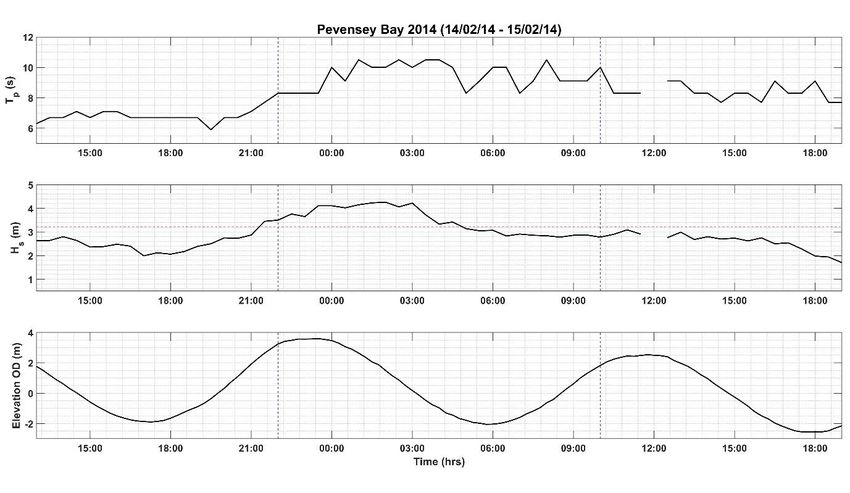
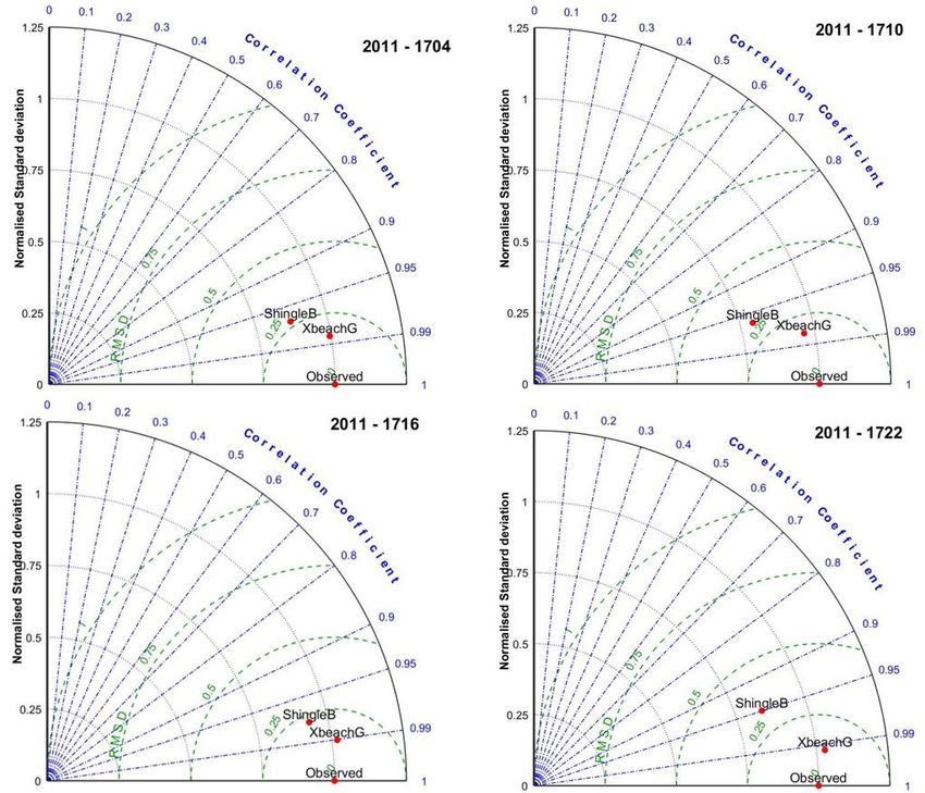
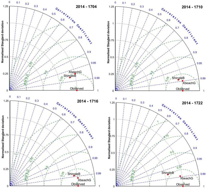
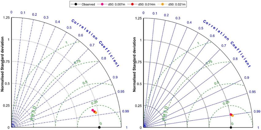
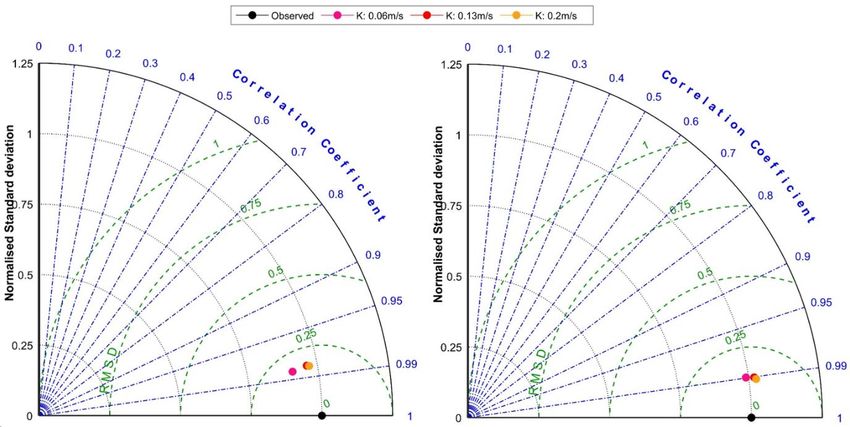
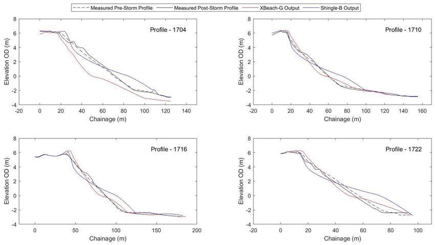
List of Figures
Fig.1: Sketch defining the relevant terms within the swash zone environment (Horn, 2002). .............. 7
Fig. 2: Spatial extent for morphological field data collection at Pevensey (brown line). Wave buoy off
the coast of Pevensey (Yellow point - 50°46.91’N 000°25.10’E)...................................................... 12
Fig. 3: Annual wave data for 2019 at Pevensey wave buoy. Occurrence of wave height (left) and
wave period (right) for each direction. ............................................................................................. 13
Fig. 4: Management profiles chosen as the focus of the model validation in this study. ‘4c01704’,
‘4c01710’, ‘4c01716’ and ‘4c01722’ (East to West). ....................................................................... 15
Fig. 5: Summary of the incident wave climate and tidal regime across the 2011 storm event. Dashed
vertical blue lines indicate the model simulation period (21:00 12/12/11 to 09:00 13/12/11) and the
dashed horizontal red line indicates the storm alert threshold at the Pevensey Bay wave buoy of 3.21m
........................................................................................................................................................ 17
Fig. 6: Morphological response of the gravel barrier at Pevensey Bay due to the 2011 storm event.
Left-hand panels indicate pre-storm and post-storm profiles, while right-hand panels demonstrate
respective bed level change of each profile. The 4 rows of panels represent the spatial distribution of
profiles across Pevensey Bay, from 1704 in the east (top row) down to 1722 in the west (bottom row).
........................................................................................................................................................ 18
Fig. 7: Summary of the incident wave climate and tidal regime across the 2014 storm event. Dashed
vertical blue lines indicate the model simulation period (22:00 14/02/14 to 10:00 15/02/14). The
dashed horizontal red line indicates the storm alert threshold at the Pevensey Bay wave buoy of
3.21m. The missing wave data outside of the simulation period indicates flagged data in the CCO time
series. .............................................................................................................................................. 19
Fig. 8: Morphological response of the gravel barrier at Pevensey Bay due to the 2014 storm event.
Left-hand panels indicate pre-storm and post-storm profiles and right-hand panels demonstrate
respective bed level change of each profile. The 4 rows of panels represent the spatial distribution of
profiles across Pevensey Bay, from 1704 in the east (top row) down to 1722 in the west (bottom row).
All elevations are converted to ordnance datum (OD). ..................................................................... 20
Fig. 9: Framework for output profile of Shingle-B model (HR Wallingford, 2018)........................... 23
Fig. 10: Beach profiles at 4 locations across the frontage of Pevensey Bay, 1704 (top left), 1710 (top
right), 1716 (bottom left) and 1722 (bottom right). Measured pre-storm profile, measured post-storm
profile, XBeach-G output profile and Shingle-B output profile for each location. In each scenario the
back barrier marks the 0m chainage point. MHWS mark is 3.88m (OD) and the MLWS mark is -
2.82m (OD). .................................................................................................................................... 29
Fig. 11: Summarising the skill of XBeach-G and Shingle-B to predict morphological evolution across
the frontage of Pevensey Bay using a Taylor Diagram. For the purpose of the Taylor Diagram,
Standard Deviation (STD) and Root Mean Square Difference (RMSD) have been normalised. ........ 31
Fig. 12: Beach profiles at 4 locations across the frontage of Pevensey Bay in response to the 2014
storm event, 1704 (top left), 1710 (top right), 1716 (bottom left) and 1722 (bottom right). Measured
pre-storm profile, measured post-storm profile, XBeach-G output profile and Shingle-B output profile
for each location. In each scenario the back barrier marks the 0m chainage point. MHWS mark is
3.88m (OD) and the MLWS mark is -2.82m (OD). .......................................................................... 32
Fig. 13: Taylor Diagram summarising the skill of XBeach-G and Shingle-B to predict morphological
evolution across the frontage of Pevensey Bay. For the purpose of the Taylor Diagram, Standard
Deviation (STD) and Root Mean Square Difference (RMSD) have been normalised. ....................... 34
Fig. 14: Comparison of accretion and erosion volumes for measured and simulated storm events for
both XBeach-G (purple) and Shingle-B (red). Black line indicates measured erosion/accretion is equal
to modelled. XBeach-G output profile 1704 for the 2014 storm event is not contained in the figure.. 35
Fig. 15: Run-up elevations using the EurOtop (2007) formula (grey bar) for model comparison, along
with model approximations from XBeach-G (red bar) and Shingle-B (blue bar) for validation. The top

 vi

plot represents the 2011 storm event and the bottom plot represents the 2014 storm event. Transparent
sections of the XBeach-G and Shingle-B bars indicate the input water level in the model, to identify
relative wave run-up elevations. For XBeach-G the maximum tide and surge level was defined at
3.23m for 2011 and 3.6m for the 2014 storm event. For Shingle-B a still water level (SWL) of 1.5m
was used. ......................................................................................................................................... 37
Fig. 16: XBeach-G output profiles from the 2011 storm event simulation at two profile locations at
Pevensey Bay (1710 and 1716) along with pre-storm and post-storm measured profiles. Top panel
represents profile 1710 and the bottom panel represents 1716. Different output profiles indicate
varying grain size (d50 - m) used to run each model simulation as part of the sensitivity analysis. .... 40
Fig. 17: Summary of statistical skill parameters for model simulations in the grain size (d50 - m)
sensitivity analysis. Left panel represents profile 1710 and right panel represents profile 1716. For the
purpose of the Taylor Diagram, Standard Deviation (STD) and Root Mean Square Difference
(RMSD) have been normalised. ....................................................................................................... 41
Fig. 18: XBeach-G output profiles from the 2011 storm event simulation at two profile locations at
Pevensey Bay (1710 and 1716) along with pre-storm and post-storm measured profiles. Top panel
represents profile 1710 and the bottom panel represents 1716. Different output profiles indicate
varying hydraulic conductivity (K - ms − 1) used to run each model simulation as part of the
sensitivity analysis........................................................................................................................... 43
Fig. 19: Summary of statistical skill parameters for model simulations in the sensitivity study of
hydraulic conductivity (K - ms − 1). Left panel represents profile 1710 and right panel represents
profile 1716. For the purpose of the Taylor Diagram, Standard Deviation (STD) and Root Mean
Square Difference (RMSD) have been normalised. .......................................................................... 44
Fig. 20: Summary of full XBeach-G sensitivity analysis for both grain size (d50) and hydraulic
conductivity (K) at four profile locations across Pevensey Bay for the 2011 storm event. The model
performance scale is a BSS plotted on the z-axis for each of the scenarios ran; skill scores are
normalised for the purpose of this figure. BSS’ for these simulations ranged from -2.57 to 0.71. ...... 45
Fig. 21: Comparison of model output profiles from the sediment friction factor sensitivity analysis for
locations 1710 (top panel) and 1716 (bottom panel). All other input parameters remain the same as the
validation section............................................................................................................................. 46
Fig. 22: Maximum velocity profiles for each fs input, computed by XBeach-G. Top panel represents
profile 1710 and bottom profile represents profile 1716. Black line (left y-axis) is the measured post-
storm profile and three dashed green lines (right y-axis) show velocity for each output chainage...... 47
Fig. 23: 2011 simulated storm event at profiles 1710 (top panel) and 1716 (bottom panel) with a
variety of input groundwater elevations for sensitivity analysis (-2m, 0m, 2m and 4m). Only the upper
section of the profile (> 3.25m elevation (OD)) is displayed in the plot due to the small variance
between model output profiles. ........................................................................................................ 48
Fig. 24: Predicted morphological response of the shingle barrier at Pevensey to unimodal (dashed
line) and bimodal (solid line) storm conditions. Top panel represents profile 1710 and the bottom
panel represents profile 1716. .......................................................................................................... 50
Fig. 25: Shingle-B simulation of the 2011 storm event at profiles 1710 (left panel) and 1716 (right
panel), under a bimodal (pink dot) and unimodal (red dot) wave spectrum. Data points summarise the
calculated statistical skill parameters for the upper section of the beach (MHWS to back barrier).
Parameters on the plot include; normalised root mean square difference, normalised standard
deviation and the correlation coefficient........................................................................................... 51
Fig. 26: Predicted morphological response of the shingle barrier with a varying input still water level
(SWL). Model is run at profile 1710 for the 2011 storm event. ......................................................... 52
Fig. 27: Longshore variability in measured bed level change at Pevensey Bay, in response to the 2014
storm event. The extent of the bed level surface is between profile 1723 in the West and 1703 in the
East, with the profiles explored in the model validation illustrated by the black triangles. Areas of red

 vii

indicate an increase in bed level (accretion) and areas of blue indicate a decrease in bed level
(erosion). ......................................................................................................................................... 59
Fig. 28: Shingle-B model bounds for input wave conditions (Hr Wallingford, 2016). ....................... 61

 viii

List of Tables
Tab. 1: Overview of model input hydrodynamic and morphological parameters for Pevensey Bay. .. 28
Tab. 2: Summary of computed statistical parameters for all profile simulations ran for the 2011 storm
event. Standard Deviation (STD), Root Mean Square Difference (RMSD), Pearson Correlation
Coefficient (ρ) and Brier Skill Score (BSS). Score ratings for Brier Skill Score include: 0.6 < BSS <
0.8 (good), 0.3 < BSS < 0.6 (reasonable), 0 < BSS < 0.3 (poor) and BSS < 0 (bad). ......................... 30
Tab. 3: Summary of computed statistical parameters for all profile simulations ran for the 2014 storm
event. Standard Deviation (STD), Root Mean Square Difference (RMSD), Pearson Correlation
Coefficient (ρ) and Brier Skill Score (BSS). ..................................................................................... 33

 ix

Glossary
2D Two Dimensional
ADV Acoustic Doppler Velocimeter
BIM Barrier Inertia Model
BSS Brier Skill Score
CCO Channel Coastal Observatory
GPS Global Positioning System
MHWS Mean High Water Springs
MLWS Mean Low Water Springs
MSG Mixed Sand-Gravel
OD Ordanance Datum
PCDL Pevensey Coastal Defence Ltd
RMSD Root Mean Square Difference
RTK-GPS Real Time Kinematic Global Positioning System
SAC Special Area of Conservation
SSSI Site of Specific Scientific Interest
STD Standard Deviation
SWL Still Water Level

 x

Chapter 1: Introduction
1.1 Background

At least 12% of the UK population are said to inhabit low elevation coastal zones (

the boundary conditions are carefully considered (McCall, 2015; HR Wallingford, 2016).
Parametric (Shingle-B) models differ in the method to process-based (XBeach-G) model, as
the former are fundamental built on empirical relationships gained through data observations;
whereas processes in the latter are described by a set of theoretical equations (Roelvink and
Reniers, 2012). The characteristics of a gravel beach vary considerably between each
location; depending on sediment properties, wave exposure and human intervention.
Constructing a model to describe these dynamic processes whilst ensuring its applicability
across a wide variety of gravel beach states has proved complicated in previous years; yet the
demand an effective solution continues to grow.

The gravel barrier along the coast at Pevensey bay plays a major role in protecting the socio-
economic and environmental value situated on the landward side of the beach. This coupled
with a net loss of sediment on the beach from West to East, is exacerbated by the construction
of hard engineered defences and Sovereign Harbour at Eastbourne; which facilitates the
erosion of the beach face downdrift in front of Pevensey (Sutherland and Thomas, 2011).
Regular nourishment of the shingle beach aims to counteract this issue by maintaining the
crest elevation to between 6m and 6.5 (OD); whilst still preserving the recreational
significance. With this sediment either bypassed from the Western side of the harbour on a
regular basis or less frequently dredged offshore; it is argued that this is an increasingly
unsustainable coastal defence technique, as much of the South Coast of England is battling
with a net loss of sediment (Moses and Williams, 2008). If the models in this study prove to
be suitable in predicting barrier evolution at Pevensey, then the information could be used to
supplement further decision making and provide a more efficient management strategy for
the region.

1.2 Aims and Objectives

The principal aim of this study is to assess the suitability of parametric and process-based
models, for cross-shore barrier profile evolution in response to storm events at Pevensey Bay.
In order to effectively address this aim, the following objectives have been set out:

1) Understand the current state of knowledge surrounding shoreline evolution on gravel
barriers and highlight the fundamental properties which govern sediment transport and
morphodynamic response to storm events.
2) Simulate previous storm events at Pevensey Bay using the parametric and process-based
models and validate the predicted morphological response using accompanying beach profile

 2

data collected by the Channel Coastal Observatory.
3) Explore the sensitivity of both models to input boundary conditions, such as morphological
parameters and bimodality in the wave spectrum to assess the model’s applicability to
simulate shoreline evolution in response to storms at Pevensey.

 3

Chapter 2: Literature Review
Coastal morphodynamics is a term used to describe the evolution of the shoreline as a
function of hydrodynamic forcing and resultant sediment transport (Voulgaris et al., 1999).
Thorough knowledge of the physical processes which define this relationship are required, to
effectively determine the governing equations and boundary conditions when modelling
shoreline evolution. Along sandy coastlines these processes are well understood, with
transport mechanisms and morphological responses relating to two key governing factors;
combined tidal-wave energy and sediment size (Short and Wright, 1983). However, the
introduction of hydraulic conductivity and swash zone hydrodynamics on a gravel beach
creates differing morphodynamic regimes; which have received comparatively little research
focus (Pontee et al., 2004; Buscombe and Masselink, 2006). This section will go onto review
the current knowledge of the processes which underpin shoreline evolution on a gravel beach;
and the extent to which these principles have been applied to modelling approaches in this
environment.

2.1 Gravel Beach Origins

Gravel beaches tend to occur in wave dominated, mid to upper latitude regions of glacial
origin (Forbes et al., 1991). Extending approximately 1000km around the coastline and
constituting approximately one third of total UK beaches (Fuller and Randall, 1988; Poate et
al., 2012). Specific to the gravel beaches of East Sussex explored in this study; sediment is
said to have been derived from both an offshore supply during the Pleistocene epoch, as well
as the erosion of chalk cliffs due the Holocene transgression (Jennings and Smyth, 1990). The
formation of these beaches is governed by the orientation of incident wave energy;
subdividing gravel beaches into drift or swash aligned (Austin and Masselink, 2006; DEFRA,
2008). Grain sizes on gravel beaches can be categorised into; granular material (2mm to 4
mm), pebbles (4mm to 64mm) and cobbles (64mm to 256mm) (Carter and Orford, 1993; van
Rijn and Sutherland, 2011). In the UK, the composition of gravel beach sediment varies
drastically at each location; therefore, a general term ‘shingle’ is used to describe the range
from pure gravel to a mixed composite beach (Powell, 1990).

2.2 Gravel Beach Morphodynamics

Gravel beaches typically exhibit features comparable to that of a reflective beach profile
under the Wright and Short (1984) beach classification framework. In stark contrast to a

 4

wider and flat dissipative sandy beach; an increased grain size can sustain a far steeper
profile, containing a number of morphological features which include a step, cusps and a
berm at the top of the beach (Austin and Masselink, 2006). The variability of sediment
composition on gravel beaches coupled with differing tidal regimes generates inconsistencies
in these morphological features between locations. Pure gravel beach profiles are highly
reflective with typically steep slopes of tan β = 0.1 to 0.25. In contrast to this, as with most
shingle beaches around the UK, the presence of a larger tidal range and addition of finer
sediment acts to alter the morphology. Hydraulic sorting of sediment leads to a flatter
dissipative foreshore (low-tide terrace) made up of the fine sand, with a steep gravel berm
leading up to the backshore resembling a more reflective domain; known as a composite
beach (Carter and Orford, 1993; Jennings and Shulmeister, 2002).

The hydrodynamics and sediment transport on gravel beaches is generally concentrated
within a narrow cross shore zone (Buscombe and Masselink, 2006). With an abrupt reduction
in depth, plunging or surging breakers dissipate the entirety of their peak incident wave
energy at the shoreline; through a combination of swash zone run up and percolation into the
unsaturated gravel profile (Stutz et al., 1998). The latter plays a key role in establishing wave
asymmetry in the swash zone and a subsequent reduction in backwash volume
(cf. Section 2.3). Which has been attributed to the onshore transport of coarse-grained
material and formation of a berm in the upper beach (Turner and Masselink, 1998).
Contrary to sediment transport on wide dissipative beaches being in part influenced by
infragravity oscillations; steeper gravel beaches are dominated by swash motions at incident
and subharmonic frequencies (Miles and Russel, 2004; McCall, 2015). On the contrary to this
however, Bertin et al (2018) indicates that lower frequency infragravity waves make a
significant contribution to wave run-up on gravel beaches, as incident band energy is
infiltrated into the profile. The development of infragravity waves in shallow, wide nearshore
zones has been associated with the offshore transport of sediment; due to the additional
stresses these standing edge waves have on suspended sediment (Aagaard and Greenwood,
2008). The absence of this phenomena on gravel beaches has a profound effect, further
contributing to the net onshore transport of sediment.

Sediment transport in the narrow gravel beach swash zone is almost exclusively attributed to
asymmetric wave action; with insignificant effects of tidal or residual current (van Rijn and
Sutherland, 2011). The mode of transport is, however, highly dependent of the composition
of sand/gravel present in the sample (Buscombe and Masselink, 2006). Changes in boundary

 5

layer flow, friction angle and protrusion of grains are directly linked to sediment
heterogeneity and have been demonstrated to influence sediment transport regimes on mixed
gravel beaches (Kuhnle, 1993; Mason and Coates, 2001). Wave asymmetry describes the
ratio of a larger uprush to backwash velocity in the swash zone; the former reaching
magnitudes of 3 m/s in more energetic wave climates. The critical threshold for motion of
grain sizes in the range of 5 to 200mm, has been estimated at 1.6 m/s and is therefore often
exceeded by the uprush of wave bores (Walker et al., 1991). A consequence of this being, the
capability of a gravel beach to transport a large amount of sediment in the cross-shore
direction during single storm events, most notably in the form of berm overtopping and
rollback (Poate et al., 2012). Due to large grain sizes, high fall velocity and shallow depths in
the swash zone; sediment transport is known to be bedload in the form of sliding and rolling
(Carter and Orford, 1993; McCall, 2015). Intergranular collisions have also been
demonstrated to have an effect the dispersion of sediment on the steep gravel beach face and
have also played an important role in monitoring gravel transport (Rouse, 1997).

2.3 Hydraulic Conductivity and Groundwater Exchange

Larger grain sizes present on a gravel beach create a permeable surface allowing the vertical
exchange of water (She et al., 2006). The ease at which water flows through porous spaces
between grains occurs is defined as hydraulic conductivity (K); for unsaturated gravel
beaches this value is in the range of 1 - 10 cm/s (Horn, 2002). As with many shingle beaches
around the UK, the presence of sand (related to sorting) has a profound effect on the
hydraulic conductivity; where an increase in sand content of 30-40% has been shown to
reduce K to ≈ 0.01 cm/s (She et al, 2006). As a consequence, models which effectively
describe sediment dynamics on impermeable sandy beaches perform poorly when applied to
shingle environments. Therefore, as the importance of gravel beaches is becoming more
apparent, research has been directed towards understanding water exchange on permeable
beach surfaces; which can be used to adapt existing models. Horn and Li (2006) have
demonstrated the sensitivity of gravel beach models, to an additional hydraulic conductivity
term, in particular surrounding the development of the upper beach berm.

The beach ground water system is defined as a shallow, unconfined aquifer where pore water
pressures below the water table are equal or greater than atmospheric (Fig.1). Unlike a
common deep aquifer where an impermeable surface marks the upper boundary, the water
table is a dynamic surface which oscillates in response to the infiltration-exfiltration of tides

 6

and swash (Horn, 2002). The elevation of the water table has long been considered a
fundamental contributor to swash zone sediment transport. Original concepts from Grant
(1948) are still widely used in the subject and state that a low water table allows the
infiltration of surface water into unsaturated sediment, encouraging accretion. Despite this
concept, applying knowledge of groundwater dynamics to gravel beach modelling has only
more recently been established (Masselink et al., 2009).

 Fig.1: Sketch defining the relevant terms within the swash zone environment (Horn, 2002).

Seepage of a wave uprush into the permeable gravel surface is key in establishing wave
asymmetry characteristic on a gravel beach, which as previously mentioned is attributed to
onshore sediment movement and berm formation. Research in recent decades has identified
two key effects of infiltration-exfiltration flow interactions on a gravel beach face. Infiltration
of water into the profile reduces the thickness of the boundary layer resulting in turbulence
closer to the bed, this increase in bed shear stress enhances the likeliness of sediment
mobilisation. Whereas the reverse occurs during exfiltration, a thickening of the boundary
layer as water seeps out of the surface; reducing near bed velocity and shear stresses. The net
effect of this process is the onshore transport of sediment up the beach face (Butt et al., 2001;
Masselink et al., 2009). Despite this, an upwards pressure gradient during exfiltration reduces
the effective weight of the upper layer acting to increase the offshore movement of sediment.

 7

It is however considered that enhancing bed shear stress plays a more dominant role in
determining the transport regime; therefore, the primary effect of infiltration-exfiltration on
gravel beaches is the onshore movement of sediment (Turner and Masselink, 1998; van Rijn
and Sutherland, 2011).

2.4 Measuring Sediment Transport on Gravel Beaches

When comparing to sandy dissipative beaches, gravel beaches provide a harsh environment
for data collection; with a steep beach face and energetic wave conditions breaking at the
shoreline (Carter and Orford, 1993). Despite this, a range of techniques have been adopted to
attempt to quantify the morphodynamics. One technique used to monitor bedload gravel
transport has been the exploitation of Self-generated Noise (SGN). Collisions between grains
in the swash zone can be detected by underwater hydrophones in the nearshore zone (Rouse,
1997; Priestly et al., 2008). This passive acoustic method has demonstrated the ability to
gather higher resolution data for long time periods. Another method commonly adopted in the
field is the use of tracer pebbles to monitor the spatial and temporal distribution of sediment
(Voulgaris et al., 1999). Despite the effectiveness of this method, it is unable to capture data
on the evolution of an entire beach profile. In order to do so, morphological surveys are
undertaken at regular intervals to monitor the beach volume change; these can be carried out
as stationary GPS surveys or moored on a quadbike for a greater spatial extent (Pontee et al.,
2004). To capture the full extent of the beach on varying temporal scales, the Argus video
system has also been used. Geo-referencing images captured across storm periods to identify
changes in the morphological profile (de Alegria-Arzaburu et al., 2008). As well as this, the
use of airborne techniques such as LiDAR and Unmanned Aerial Systems are becoming
increasingly desirable as the technology becomes more easily accessible to researchers along
the coastline (Elsner et al., 2018).

Despite a range of accessible field study techniques, there was still a clear demand for an
extensive gravel beach dataset which could be used to reinforce knowledge and aid model
validation. A large-scale experiment was carried out at the Hanover wave flume in Germany
with an attempt to address this gap in knowledge. Varying wave conditions were produced
over two beach scenarios; pure gravel and a mixed beach, accompanied with a selection of
data collection equipment including pressure transducers, ADV’s (Acoustic Doppler
Velocimeter) and hydrophones. Once collected, the extensive data compilation was made
publicly available with the aim of raising our understanding of gravel beaches (de San

 8

Roman-Blanco et al., 2006). This study enabled the development of a conceptual model for
gravel beaches as well as extensive validation of existing parametric models. Following this
study there was a requirement to extend this analysis to varying MSG beach locations to test
the significance of the model validation observed.

2.5 Storm Impacts on Gravel Beaches

The ability to dissipate energy over narrow distances as described by the mechanisms above,
makes gravel beaches a desirable natural form of coastal defence (Aminti et al., 2003).
Despite this, the low-lying hinterland in close proximity behind many gravel beaches are still
vulnerable to inundation; as demonstrated by the 2013/2014 extreme storm events around SW
England (Poate et al., 2015). Understanding the extent of damage and threshold for storm
events is vital to effectively model future events and influence mitigation strategies (Burvingt
et al., 2017). Elevated run-up heights enhance the onshore transport of coarse-grained gravel,
resulting in a distinct storm profile; where a portion of material is lost from the active beach
and deposited as a storm berm (Buscombe and Masselink, 2006). Under extreme conditions,
a sequence of storm events gravel beaches may be overtopped leading to a ‘rollback’ of the
elevated barrier crest; flattening the beach profile and flooding the land behind (Sutherland
and Thomas, 2011).

The response shingle beaches to storm events has been shown to fluctuate significantly
between differing locations; being attributed to sediment characteristics, hydrodynamic
forcing and local geology. The fraction of sand within the sediment sample as previously
discussed, has a considerable effect on the transport processes (She et al., 2006) and
subsequently causes shingle beaches to act differently in response to storm events. A poorly
sorted profile will likely lead to the seaward transport of fine sand generating an offshore bar
(Bramato et al., 2012). Whereas under the same hydrodynamic conditions, a well sorted
homogenous gravel sediment composition often leads to the onshore migration of sediment
forming a storm berm around the upper beach; dependant on run-up elevations (Austin and
Masselink, 2006). In addition to this, shingle beaches response to storm events has been
shown to be highly dependent on the properties of the incident wave climate. Burvingt et al
(2017) through a cluster analysis technique, classified beach response to storms as a factor of;
wave exposure, angle of wave approach and the degree of beach embayment. Indicating that
semi exposed beaches with a significant oblique incident wave attack, were likely to
experience considerable variability in the alongshore erosion of sediment. Similarly, in an

 9

analysis of beach response around the UK coastline to the 2013/2014 storms; Scott et al
(2016) highlighted the concept of rotational beach response for semi exposed gravel beaches
and a significantly landward retreat of the profile for many exposed coastlines.

Understanding the response of gravel profiles to storm events is key to establish the future
vulnerability of a beach and has therefore gathered increased attention. It has been shown the
recovery process of a gravel beach profile is longest in response to sequence of storm events
as opposed to an individual period of extreme conditions (Poate et al., 2015), with some
beaches taking a number of years to recover its sediment after continued wave exposure.
Clustered storm events are considered to pose the largest threat to coastal regions, as gravel
beaches remain vulnerable to wave run-up and continued erosion if sediment is not
replenished.

2.6 Modelling Gravel Beaches

Modelling the evolution of the beach profile on gravel beaches can take two fundamental
forms; an empirical/parametric or process-based model. Firstly, parametric models are built
upon empirical relationships identified through data observation (Roelvink and Reniers,
2012). Input parameters which typically involve the incident wave conditions (wavelength
and period) and sediment data, are related by a set of equations which estimate the output
profile. Empirical equations for beach environments usually include, run up, near bed orbital
velocity and critical bed shear stress (McCall, 2015).

Through extensive physical modelling at HR Wallingford, Powell (1990) developed the first
major parametric modelling system for gravel beaches. ‘SHINGLE’ predicts the evolution of
a beach profile based on three key relationships; ratio of wave height to sediment size, wave
steepness and ratio of wave power to sediment size. This model has been a key tool used by
the Environment Agency to model the evolution of gravel barrier crest on shingle beaches
around the UK, investigating the potential for overtopping and rollback (DEFRA, 2008).
Despite this, the bimodal wave spectrum characteristic of beaches in the English Channel is
not within the capabilities of SHINGLE. This meant that crest erosion and flatter profile
associated with larger swell waves was not well modelled (van Rijn and Sutherland, 2011).
This led to the generation of Shingle-B to equate for these wave climates (HR Wallingford,
2016). Another empirical model used in much of the coastal management work around the
UK is the Barrier Inertia Model (BIM); which predicts the likely of overwash on a gravel
barrier (Bradbury, 2000). Extensive laboratory and field data defined an empirical

 10

relationship between the wave steepness (Sw) and properties of the gravel barrier (freeboard
and cross-sectional area). Despite its use by many coastal engineers, the suitability of the
BIM to effectively predict overwash potential may be limited due to validation constrained to
one site (Hurst Spit), as well as no consideration of the effect of beach slope and wave run-up
elevations.

In contrast to this, a process-based model attempts to understand the underlying physical
principles occurring within the beach system, to accurately recreate the processes across a
range on environments. Such models tend to solve some variation of the non-linear shallow
water equations to describe the hydrodynamics, the momentum equation for swash zone
dynamics (Kobayashi and Wurjanto, 1992) and its subsequent effects on bed shear stress, in
the form of the shield’s parameter for bed load transport (Roelvink and Reniers, 2012).
Attempts to model gravel beaches have been made in the past with varying success; Van Rijn
and Sutherland (2011) applied the CROSMOR2008 model, which solves the wave energy
equation for each individual wave in the swash zone. Additionally, ‘XBeach’ which was
created originally for sandy coastlines (Roelvink et al., 2009) has been altered and applied to
gravel beaches (Alegria-Arzaburu et al., 2011; Jamal et al., 2014). Such research has
uncovered the importance of additional inclusive terms into these process-based models for
gravel beaches; surrounding groundwater elevation and infiltration-exfiltration exchange
(Horn and Li, 2006; McCall, 2015). To rectify this complication; McCall (2015) formulated
XBeach-G, solving wave by wave flow and groundwater exchange to efficiently model
gravel beaches. This model was however created for pure gravel beaches, therefore its
suitability to a mixed sand-gravel composition characteristic of Pevensey is explored to a
lesser extent.

 11

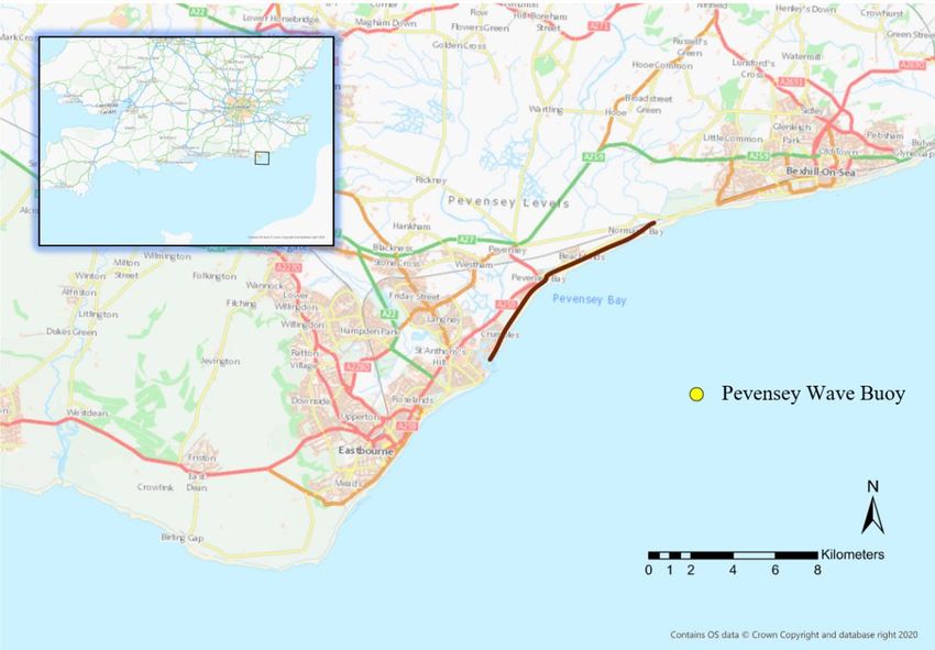
Chapter 3: Methodology
3.1 Study Site

3.1.1 Overview

The gravel beach which forms the focus of this study is Pevensey Bay, East Sussex. A 9km
long shingle barrier extending from the Sovereign Harbour in the West, across the frontage of
Pevensey, to Cooden at the eastern end of the beach (Fig. 2). The natural shingle barrier is the
primary mechanism for coastal defence in the area; with key socio-economic and
environmental assets situated behind it. The Pevensey Levels is a low-lying section of
marshland inland of the gravel beach; containing an abundant community of birds and plant
life which are extremely vulnerable to inundation of saltwater water. Under Natura 2000,
Pevensey Levels are designated as a Site of Special Scientific Interest (SSSI) and Special
Area of Conservation (SAC ); therefore, must be protected against any potential threat of
flooding (Environment Agency, 2010). The heavily developed coastline across Pevensey Bay
means in excess of 18600 properties (Welch, 2019), an array campsites and key railway line
would all be exposed to flooding if the barrier were to be breached (East Sussex County
Council, 2014).

 Fig. 2: Spatial extent for morphological field data collection at Pevensey (brown line). Wave buoy off the coast
 of Pevensey (Yellow point - 50°46.91’N 000°25.10’E).

 12

The composition of sediment along Pevensey bay resembles that of a classic mixed sand-
gravel composite beach profile. A low tide terrace consisting of finer grain sediment (d50 <
2mm) fronted by a steeper high tide beach face made up of gravel and cobbles (d50 > 5mm)
(van Rijn and Sutherland, 2011). For the purpose of this study, a single grain size d50 =
14mm is assumed constant across the entirety of the beach profile at Pevensey Bay (HR
Wallingford, 2016). Despite this, the heterogeneity of sediment across the gravel barrier
varies considerably; with the fraction of fine sediment in the surface layer being a function of
hydrodynamic forcing and beach recharge events (Dornbusch et al., 2005).

The tidal range in the area is typically between -2.8m and 3.8m OD and crest elevation of the
Pevensey barrier is +6.5m OD. This results in flooding events being highly dependent on the
constructive interference of wave run-up, storm surge and high tides. The incident wave
climate at Pevensey (Fig. 3) consists of longer period swell events arriving from the
southwest direction up the English Channel, or shorter period wind waves from the east
originating from a limited fetch length (Sutherland and Thomas, 2009). Despite the wave
spectrum at Pevensey Bay experiencing less bimodality than other locations at the Western
end of the English Channel. It has been observed that significant Atlantic swell events have
the potential to propagate to the Eastern end of the channel resulting in long period storm
waves arriving at Pevensey amongst short period storms (Polidoro et al., 2018).

 Fig. 3: Annual wave data for 2019 at Pevensey wave buoy. Occurrence of wave height (left) and wave period
 (right) for each direction.

 13

3.1.2 Current Beach Management

Beginning in the mid-20th century, the coastline along Pevensey Bay has been engineered
using a variety of techniques. 150 wooden groynes have been constructed along the beach in
an attempt to mitigate against the longshore drift of sediment from west to east, however
these have reached the end of their design life. Along with this, a series of seawalls and
rubble mound structures fronting Pevensey to protect the most vulnerable sections from
overtopping events (Sutherland and Thomas, 2011). Current management of the gravel beach
at Pevensey Bay has been contracted by the Environment Agency to Pevensey Coastal
Defence Ltd (PCDL) as part of a 25-year agreement. A more adaptive management approach
has been adopted; aiming to sustainably protect the value along the coastline against flooding
whilst carefully considering social, economic and environmental concerns (HM Government,
2018).

The primary issue at Pevensey is the associated risks of a 30,000 m3 net loss sediment
budget west to east; as the equilibrium of the breach has been unbalanced (Harvey, 2016).
This problem is exacerbated by the presence of a rubble mound breakwater constructed at the
Sovereign Harbour, trapping the natural movement of sediment and promoting downdrift
erosion in the lee of the structure (Sutherland and Thomas, 2011). The primary mitigation
aims for the PCDL is to maintain the gravel barrier to a 1 in 400-year flood protection
standard; accomplished through a combination of beach nourishment from offshore dredging
and manual bypassing of sediment around the Sovereign harbour (crest elevation +6.5m OD).
An annual average of 21,000 m3 of dredged material is deposited and 9,000 m3 is bypassed
along the coast at Pevensey (Harvey, 2016).

3.1.3 Management Profiles

The Channel Coastal Observatory (CCO) topographic survey programme for the south coast
of England, aims to gather a long-term archive of shoreline elevation data by taking bi-annual
beach profiles. The Pevensey Bay management unit ‘4cSU23’ extends from Sovereign
Harbour in the west to Bexhill in the east. Unit 4cSU23 extending around 9km across the
frontage of Pevensey Bay, is split into profiles at 150m intervals for monitoring by the CCO.
The limits of these profiles are ‘4c01672’ in the east (Bexhill) to ‘4c01729’ in the West
(Sovereign Harbour). CCO beach surveys are carried out using either Real Time Kinematic
Global Positioning System (RTK-GPS) or the higher resolution laser scanning technique. In
an attempt to understand and predict the morphological evolution across the full spatial extent

 14

at Pevensey, 4 management profiles have been chosen as the focus of this study (Fig. 4).
These profiles were identified in order to take into account the spatial variability in sediment
composition documented at Pevensey (Dornbusch et al., 2005), along with any changes in the
incident wave climate along the coast, due to refraction of waves around Beachy Head to the
west.

 Fig. 4: Management profiles chosen as the focus of the model validation in this study. ‘4c01704’, ‘4c01710’,
 ‘4c01716’ and ‘4c01722’ (East to West).

3.2 Previous Research at Pevensey Bay

The MSG beach at Pevensey ensures the morphodynamic processes will vary to that of pure
gravel (McCall et al., 2012; McCall 2015). The presence of fine sand in a gravel barrier has
been shown to, limit the infiltration of surface water into the sediment (Horn, 2002) and also
promote an offshore erosion of finer sediment during storm events (Stephane et al., 2008).
Despite this, there is still the potential for the barrier crest to be overtopped by wave action.
Demonstrated by the 1999 flooding of 50 homes along the frontage of Pevensey, where the

 15

barrier crest was flattened and overwash onto the backshore occurred (Sutherland and
Thomas, 2011).

As Pevensey Bay is currently one of the primary concerns for the Environment Agency’s
coastal management sector, it is clear there has been a variety of ongoing research into the
processes along the barrier. Sutherland and Thomas, 2011 provide a detailed summary of the
key management strategies which take place along the barrier and how the decision-making
process will evolve into the future to take a more adaptive approach. Additionally, field
study-based research has been undertaken using a variety of techniques such as pole mounted
volumetric surveys (Welch, 2019), remote sensing and aerial imaging (Stephane, 2018) to
make observations of barrier evolution. Efforts have also been taken to understand the effect
which beach nourishment at Pevensey has had on the sediment composition and the
potentially detrimental effects for beach erosion. Horn and Walton (2007) have identified the
sediment grading can change from a predominantly fine and coarse gravel upper beach, to
containing a significant fine sand fraction in response to nourishment of the profile.

Also, a modelling approach has been used to outline morphodynamic response to storms; yet
the ability to predict potential overwash and beach threshold is limited (van Rijn and
Sutherland, 2011). The process-based model ‘CROSMOR2008’ was found to be most
effective at predicting shoreline evolution under the largest storm waves; whereas the
parametric model ‘SHINGLE’ significantly overpredicted the build-up of sediment on top of
the crest. Both models used in this study were of limited suitability to storm events at
Pevensey, with CROSMOR originally developed for observing bar migration on sandy
beaches (van Rijn et al., 2003) and the SHINGLE model giving no consideration to the
potential for a bimodal wave spectrum at Pevensey (HR Wallingford, 2016). Therefore, there
is an obvious void in the knowledge of barrier evolution at Pevensey Bay and a demand for
the application of gravel beach specific models is present.

3.3 Data Observations

Hydrodynamic and morphological data acquired from the CCO is used to set up and validate
both XBeach-G and Shingle-B models, to assess their suitability to predict gravel beach
profile evolution. The storm events summarised in this section, which will be used to validate
the models, have been selected due to the energetic wave climate and subsequent sediment
loss which has occurred. The response of a gravel beach due to wave events which exceed the
storm alert threshold for prolonged periods, is of a key interest for coastal engineers looking

 16

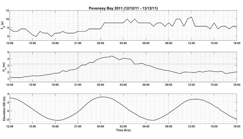
to protect coastal regions and is thus the focus of this modelling exercise. Two significant
wave events; in 2011 and 2014, have been identified from a time series of wave data, which
have complimentary pre-storm and post-storm beach profiles for model validation.

3.3.1 2011 Storm Event

On the 12th - 13th of December 2011, the gravel barrier at Pevensey Bay was exposed to a
considerable storm event (Fig. 5). Incident wave heights (Hs) in excess of 4.4m coupled with
the occurrence on a high tide (3.26m OD) led to significant erosion of the shingle profile,
with local reports of water levels reaching the crest elevation of +6.5m OD during high tide.
Fig.5 demonstrates the severity of this individual wave event, with the storm alert threshold
for significant wave height being exceeded for a duration of around 7 hours. Despite the peak
swell wave period (Tp) of 10.1s occurring after the peak of the storm; the wave run up due to
tidal and storm surge levels, coupled with Hs was significant enough to cause considerable
erosion of the upper gravel profile. Analysis of wave spectra data indicated that there was
significant bimodality in the wave climate, with a 60-70% swell component throughout the
storm event.

 Fig. 5: Summary of the incident wave climate and tidal regime across the 2011 storm event. Dashed vertical
 blue lines indicate the model simulation period (21:00 12/12/11 to 09:00 13/12/11) and the dashed horizontal
 red line indicates the storm alert threshold at the Pevensey Bay wave buoy of 3.21m

 17