State-dependent regulation of cortical processing speed via gain modulation - arXiv.org
←
→
Page content transcription
If your browser does not render page correctly, please read the page content below
State-dependent regulation of cortical processing
                                            speed via gain modulation
arXiv:2004.04190v3 [q-bio.NC] 26 Jan 2021

                                            David Wyricka and Luca Mazzucatoa,b
                                             a
                                              Department of Biology and Institute of Neuroscience, b Department of Mathematics and Physics,
                                             University of Oregon, Eugene.

                                             E-mail: lmazzuca at uoregon dot edu

                                            Abstract: To thrive in dynamic environments, animals must be capable of rapidly and
                                            flexibly adapting behavioral responses to a changing context and internal state. Examples of
                                            behavioral flexibility include faster stimulus responses when attentive and slower responses
                                            when distracted. Contextual or state-dependent modulations may occur early in the cor-
                                            tical hierarchy and may be implemented via top-down projections from cortico-cortical or
                                            neuromodulatory pathways. However, the computational mechanisms mediating the effects
                                            of such projections are not known. Here, we introduce a theoretical framework to classify
                                            the effects of cell-type specific top-down perturbations on the information processing speed
                                            of cortical circuits. Our theory demonstrates that perturbation effects on stimulus process-
                                            ing can be predicted by intrinsic gain modulation, which controls the timescale of the circuit
                                            dynamics. Our theory leads to counter-intuitive effects such as improved performance with
                                            increased input variance. We tested the model predictions using large-scale electrophysio-
                                            logical recordings from the visual hierarchy in freely running mice, where we found that a
                                            decrease in single-cell intrinsic gain during locomotion led to an acceleration of visual pro-
                                            cessing. Our results establish a novel theory of cell-type specific perturbations, applicable
                                            to top-down modulation as well as optogenetic and pharmacological manipulations. Our
                                            theory links connectivity, dynamics, and information processing via gain modulation.
Contents

1 Introduction                                                                           1

2 Methods                                                                                3
  2.1 Spiking network model                                                              3
  2.2 Mean field theory                                                                  6
  2.3 Experimental data                                                                  9
  2.4 Stimulus decoding                                                                  9
  2.5 Firing rate distribution match                                                    10
  2.6 Single-cell gain                                                                  10
  2.7 Single-cell response and selectivity                                              10

3 Results                                                                           12
  3.1 State-dependent regulation of the network emergent timescale                  13
  3.2 Changes in cluster timescale are controlled by gain modulation                14
  3.3 Controlling information processing speed with perturbations                   16
  3.4 Gain modulation regulates the network information processing speed            17
  3.5 Physiological responses to perturbations                                      20
  3.6 Changes in single-cell responses cannot explain the effects of perturbations
      on evoked activity                                                            20
  3.7 Locomotion decreases single-cell gain and accelerates visual processing speed 22

4 Discussion                                                                         25
  4.1 Metastable activity in cortical circuits                                       25
  4.2 Linking metastable activity to flexible cognitive function via gain modulation 26
  4.3 Alternative models of gain modulation                                          27
  4.4 Physiological mechanisms of gain modulation                                    27
  4.5 Locomotion and gain modulation                                                 29

5 Acknowledgements                                                                      30

1   Introduction

Animals respond to the same stimulus with different reaction times depending on the con-
text or the behavioral state. Faster responses may be elicited by expected stimuli or when
the animal is aroused and attentive [1]. Slower responses may occur in the presence of
distractors or when the animal is disengaged from the task [2–4]. Experimental evidence
suggests that neural correlates of these contextual modulations occur early in the cortical
hierarchy, already at the level of the primary sensory cortex [5, 6]. During the waking

                                           –1–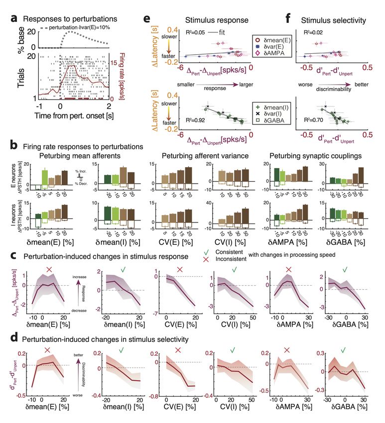
state, levels of arousal, attention, and task engagement vary continuously and are associ-
ated with ongoing and large changes in the activity of neuromodulatory systems [7–9] as
well as cortico-cortical feedback pathways [10–14]. Activation of these pathways modulate
the patterns of activity generated by cortical circuits and may affect their information-
processing capabilities. However, the precise computational mechanism underlying these
flexible reorganizations of cortical dynamics remains elusive.
     Variations in behavioral and brain state, such as arousal, engagement and body move-
ments may act on a variety of timescales, both slow (minutes, hours) and rapid (seconds or
subsecond), and spatial scales, both global (pupil diameter, orofacial movements) and brain
subregion-specific; and they can be recapitulated by artificial perturbations such as opto-
genetic, chemogenetic or electrical stimulation. These variations have been associated with
a large variety of seemingly unrelated mechanisms operating both at the single cell and at
the population level. At the population level, these mechanisms include modulations of low
and high frequency rhythmic cortical activities [15]; changes in noise correlations [16, 17];
and increased information flow between cortical and subcortical networks [15]. On a cellular
level, these variations have been associated with modulations of single-cell responsiveness
and reliability [17]; and cell-type specific gain modulation [15]. These rapid, trial-by-trial
modulations of neural activity may be mediated by neuromodulatory pathways, such as
cholinergic and noradrenergic systems [7–9, 18], or more precise cortico-cortical projections
from prefrontal areas towards primary sensory areas [10–14]. The effects of these cortico-
cortical projections can be recapitulated by optogenetic activation of glutamatergic feedback
pathways [19]. In the face of this wide variety of physiological pathways, is there a common
computational principle underlying the effects they elicit on sensory cortical circuits?
     A natural way to model the effect of activating a specific pathway on a downstream cir-
cuit is in the form of a perturbation to the downstream circuit’s afferent inputs or recurrent
couplings [20, 21]. Here, we will present a theory explaining how these perturbations con-
trol the information-processing speed of a downstream cortical circuit. Our theory shows
that the effects of perturbations that change the statistics of the afferents or the recurrent
couplings can all be captured by a single mechanism of action: intrinsic gain modulation,
where gain is defined as the rate of change of the intrinsic input/output transfer function of
a neuron measured during periods of ongoing activity. Our theory is based on a biologically
plausible model of cortical circuits using clustered spiking network [22]. This class of mod-
els capture complex physiological properties of cortical dynamics such as state-dependent
changes in neural activity, variability [23–27] and information-processing speed [20]. Our
theory predicts that gain modulation controls the intrinsic temporal dynamics of the cor-
tical circuit and thus its information processing speed, such that decreasing the intrinsic
single-cell gain leads to faster stimulus coding.
     We tested our theory by examining the effect of locomotion on visual processing in
the visual hierarchy. We found that locomotion decreased the intrinsic gain of visual cor-
tical neurons in the absence of stimuli in freely running mice. The theory thus predicted
a faster encoding of visual stimuli during running compared to rest, which we confirmed
in the empirical data. Our theoretical framework links gain modulation to information-
processing speed, providing guidance for the design and interpretation of future manipu-

                                            –2–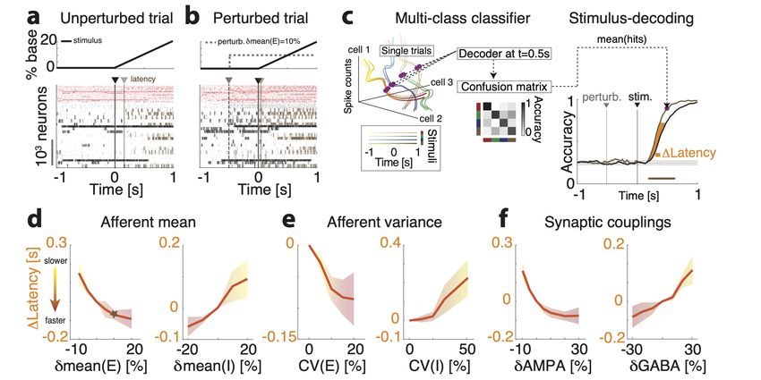
lation experiments by unifying the changes in brain state due to behavior, optogenetic, or
pharmacological perturbations, under the same shared mechanism.

2     Methods

2.1    Spiking network model
Architecture. We modeled the local cortical circuit as a network of N = 2000 excitatory
(E) and inhibitory (I) neurons (with relative fraction nE = 80% and nI = 20%) with
random recurrent connectivity (Fig. 2). Connection probabilities were pEE = 0.2 and
pEI = pIE = pII = 0.5. Nonzero synaptic weights from pre-synaptic neuron j to post-
                                    √
synaptic neuron i were Jij = jij / N , with jij sampled from a gaussian distribution with
mean jαβ , for α, β = E, I, and standard deviation δ 2 . E and I neurons were arranged in
p clusters. E clusters had heterogeneous sizes drawn from a gaussian distribution with a
mean of NEclust = 80 E-neurons and 20% standard deviation. The number of clusters was
then determined as p = round(nE N (1 − nbgr )/NEclust ), where nbgr = 0.1 is the fraction
of background neurons in each population, i.e., not belonging to any cluster. I clusters
had equal size NIclust = round(nI N (1 − nbgr /p). Clusters were defined by an increase
in intra-cluster weights and a decrease in inter-cluster weights, under the constraint that
the net input current to a neuron would remain unchanged compared to the case without
clusters. Synaptic weights for within-cluster neurons where potentiated by a ratio factor
  +
Jαβ . Synaptic weights between neurons belonging to different clusters were depressed by
           −
a factor Jαβ  . Specifically, we chose the following scaling: JEI+
                                                                     = p/(1 + (p − 1)/gEI ),
                                 −                 −
JIE = p/(1 + (p − 1)/gIE ), JEI = JEI /gEI , JIE = JIE /gIE and Jαα
  +                                     +                 +             − = 1 − γ(J + − 1)
                                                                                       αα
for α = E, I, with γ = f (2 − f (p + 1))−1 , where f = (1 − nbgr )/p is the fraction of E
neurons in each cluster. Within-cluster E-to-E synaptic weights were further multiplied
by cluster-specific factor equal to the ratio between the average cluster size NEclust and the
size of each cluster, so that larger clusters had smaller within-cluster couplings. We chose
network parameters so that the cluster timescale was 100 ms, as observed in cortical circuits
[20, 25, 28]. Parameter values are in Table 1.
Neuronal dynamics. We modeled spiking neurons as current-based leaky-integrate-and-fire
(LIF) neurons whose membrane potential V evolved according to the dynamical equation
                                  dV    V
                                     =−    + Irec + Iext ,
                                  dt    τm
where τm is the membrane time constant. Input currents included a contribution Irec
coming from the other recurrently connected neurons in the local circuit and an external
current Iext = I0 + Istim + Ipert (units of mV s−1 ). The first term I0 = Next Jα0 rext (for
α = E, I) is a constant term representing input to the E or I neuron from other brain
areas and Next = nE N pEE ; while Istim and Ipert represent the incoming sensory stimulus
or the various types of perturbation (see Stimuli and perturbations below). When V hits
threshold Vαthr (for α = E, I), a spike is emitted and V is then held at the reset value V reset
for a refractory period τref r . We chose the thresholds so that the homogeneous network
                  ±
(i.e.,where all Jαβ  = 1) was in a balanced state with average spiking activity at rates

                                             –3–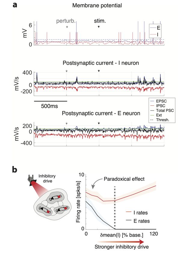
Model parameters for clustered network simulations
 Parameter       Description                                                          Value
                                                   √
 jEE             mean E-to-E synaptic weights × N                                     0.6 mV
                                                  √
 jIE             mean E-to-I synaptic weights × N                                     0.6 mV
                                                  √
 jEI             mean I-to-E synaptic weights × N                                     1.9 mV
                                                  √
 jII             mean I-to-I synaptic weights × N                                     3.8 mV
                                                   √
 jE0             mean E-to-E synaptic weights × N                                     2.6 mV
                                                  √
 jI0             mean I-to-I synaptic weights × N                                     2.3 mV
 δ               standard deviation of the synaptic weight distribution               20%
   +
 JEE             Potentiated intra-cluster E-to-E weight factor                       14
   +
 JII             Potentiated intra-cluster I-to-I weight factor                       5
 gEI             Potentiation parameter for intra-cluster I-to-E weights              10
 gIE             Potentiation parameter for intra-cluster E-to-I weights              8
 rext            Average baseline afferent rate to E and I neurons                    5 spks/s
 VEthr           E-neuron threshold potential                                         1.43 mV
 VIthr           I-neuron threshold potential                                         0.74 mV
 V reset         E- and I-neuron reset potential                                      0 mV
 τm              E- and I-neuron membrane time constant                               20 ms
 τref r          E- and I-neuron absolute refractory period                           5 ms
 τs              E- and I-neuron synaptic time constant                               5 ms

             Table 1. Parameters for the clustered network used in the simulations.

(rE , rI ) = (2, 5) spks/s [20, 22]. Post-synaptic currents evolved according to the following
equation
                                                  N
                                dIrec           X     X
                           τsyn       = −Irec +   Jij   δ(t − tk ) ,
                                 dt
                                                 j=1      k

where τs is the synaptic time constant, Jij are the recurrent couplings and tk is the time of
the k-th spike from the j-th presynaptic neuron. Parameter values are in Table 1.
     Sensory stimuli. We considered two classes of inputs: sensory stimuli and perturbations.
In the “evoked” condition (Fig. 4a), we presented the network one of four sensory stimuli,
modeled as changes in the afferent currents targeting 50% of E-neurons in stimulus-selective
clusters; each E-cluster had a 50% probability of being selective to a sensory stimulus
(mixed selectivity). In the first part of the paper (Fig. 1-6, I-clusters were not stimulus-
selective. Moreover, in both the unperturbed and the perturbed stimulus-evoked conditions,
stimulus onset occurred at time t = 0 and each stimulus was represented by an afferent
current Istim (t) = Iext rstim (t), where rstim (t) is a linearly ramping increase reaching a value
rmax = 20% above baseline at t = 1. In the last part of the paper (Fig. 7), we introduced
a new stimulation protocol where visual stimuli targeted both E and I clusters in pairs,
corresponding to thalamic input onto both excitatory and inhibitory neurons in V1 [29–
32].. Each E-I cluster pair had a 50% probability of being selective to each visual stimulus.
If a E-I cluster pair was selective to a stimulus, then all E neurons and 50% of I neurons

                                              –4–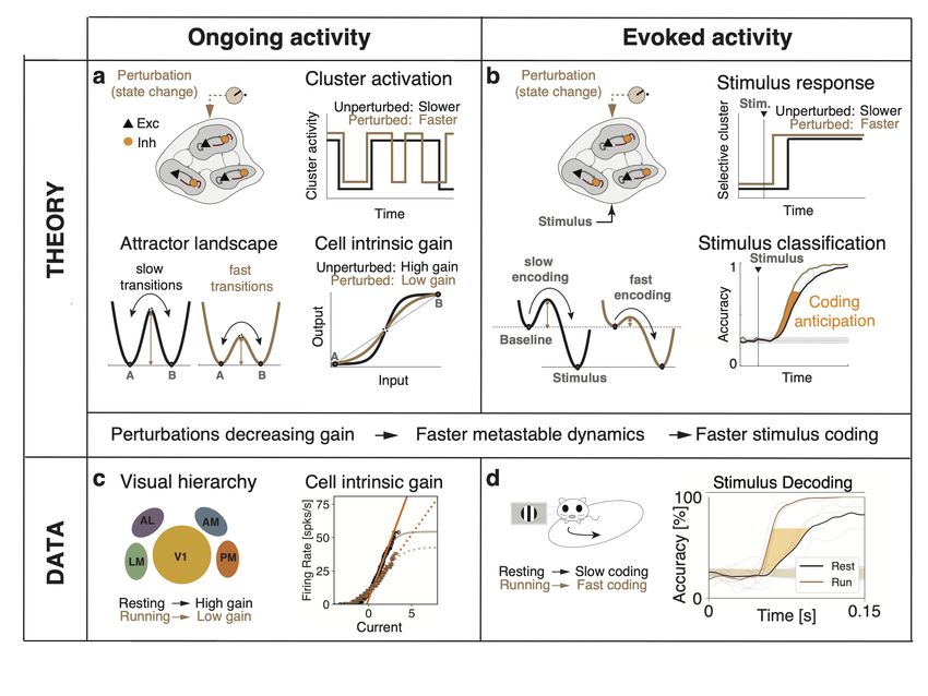
in that pair received the stimulus. The time course of visual stimuli was modeled as a
double exponential profiles with rise and decay times of (0.05,0.5)s, and peak equal to a
20% increase compared to the baseline external current.
    External perturbations. We considered several kinds of perturbations. In the per-
turbed stimulus-evoked condition (Fig. 4b, right panel), perturbation onset occurred at
time t = −0.5 and lasted until the end of the stimulus presentation at t = 1 with a constant
time course. We also presented perturbations in the absence of sensory stimuli (“ongoing”
condition, Fig. 2-3); in that condition, the perturbation was constant and lasted for the
whole duration of the trial (5s). Finally, when assessing single-cell responses to perturba-
tions, we modeled the perturbation time course as a double exponential with rise and decay
times [0.1, 1]s (Fig. 6). In all conditions, perturbations were defined as follows:

   • δmean(E), δmean(I): A constant offset Ipert = zI0 in the mean afferent currents was
     added to all neurons in either E or I populations, respectively, expressed as a fraction
     of the baseline value I0 (see Neuronal dynamics above), where z ∈ [−0.1, 0.2] for E
     neurons and z ∈ [−0.2, 0.2] for I neurons.

   • δvar(E), δvar(I): For each E or I neuron, respectively, the perturbation was a constant
     offset Ipert = zI0 , where z is a gaussian random variable with zero mean and standard
     deviation σ. We chose σ ∈ [0, 0.2] for E neurons and σ ∈ [0, 0.5] for I neurons. This
     perturbation did not change the mean afferent current but only its spatial variance
     across the E or I population, respectively. We measured the strength of these per-
     turbations via their coefficient of variability CV (α) = σα /µα , for α = E, I, where σ
     and µ = I0 are the standard deviation and mean of the across-neuron distribution of
     afferent currents.

   • δAMPA: A constant change in the mean jαE → (1+z)jαE synaptic couplings (for α =
     E, I), representing a modulation of glutamatergic synapses. We chose z ∈ [−0.1, 0.2].

   • δGABA: A constant change in the mean jαI → (1 + z)jαI synaptic couplings (for α =
     E, I), representing a modulation of GABAergic synapses. We chose z ∈ [−0.2, 0.2].

The range of the perturbations were chosen so that the network still produced metastable
dynamics for all values.
     Inhibition stabilization. We simulated a stimulation protocol used in experiments to test
inhibition stabilization (Fig. 2-1b). This protocol is identical to the δmean(I) perturbation
during ongoing periods, where the perturbation targeted all I neurons with an external
current Ipert = zI0 applied for the whole length of 5s intervals, with z ∈ [0, 1.2] and 40
trials per network and 10 networks for each value of the perturbation.
     Simulations. All data analyses, model simulations, and mean field theory calculations
were performed using custom software written in MATLAB, C and Python. Simulations in
the stimulus-evoked conditions (both perturbed and unperturbed) comprised 10 realizations
of each network (each network with different realization of synaptic weights), with 20 trials
for each of the 4 stimuli. Simulations in the ongoing condition comprised 10 different real-
ization of each network, with 40 trials per perturbation. Each network was initialized with

                                            –5–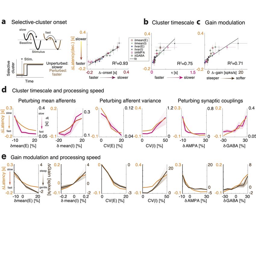
Model parameters for the reduced two-cluster network
 Parameter       Description                                                          Value
                                                  √
 jEE             mean E-to-E synaptic weights × N                                     0.8 mV
                                                  √
 jEI             mean I-to-E synaptic weights × N                                     10.6 mV
                                                  √
 jIE             mean E-to-I synaptic weights × N                                     2.5 mV
                                                 √
 jII             mean I-to-I synaptic weights × N                                     9.7 mV
                                                  √
 jE0             mean E-to-E synaptic weights × N                                     14.5 mV
                                                 √
 jI0             mean I-to-I synaptic weights × N                                     12.9 mV
   +
 JEE             Potentiated intra-cluster E-to-E weight factor                       11.2
 rext            Average baseline afferent rate to E and I neurons                    7 spk/s
 VEthr           E-neuron threshold potential                                         4.6 mV
 VIthr           I-neuron threshold potential                                         8.7 mV
 τs              E- and I-neuron synaptic time constant                               4 ms
 nbgr            Fraction of background E neurons                                     65%

Table 2. Parameters for the simplified two-cluster network used for the mean-field theory analysis
(the remaining parameters are in Table 1.

random synaptic weights and simulated with random initial conditions in each trial. Sample
sizes were similar to those reported in previous publications [20, 25, 26]. Dynamical equa-
tions for the leaky-integrate-and-fire neurons were integrated with the Euler method with
a 0.1ms step. MATLAB code to simulate the model with δvar(E) perturbation is located
at https://github.com/mazzulab/perturb_spiking_net. Code to reproduce the full set
of perturbations investigated in this paper are available upon request to the corresponding
author.

2.2   Mean field theory

We performed a mean field analysis of a simplified two-cluster network for leaky-integrate-
and-fire neurons with exponential synapses, comprising p + 2 populations for p = 2 [20, 22]:
the first p representing the two E clusters, the last two representing the background E and
the I population. The infinitesimal mean µn and variance σn2 of the postsynaptic currents
are:

                                                 p−1
               "                                                                       !              #
           √                      +         −
                                                X                    bgr     j E0
 µn = τm N nE pEE jEE          f JEE rn + JEE  (     rl + (1 − pf )rE ) +         rext − nI pEI jEI rI ,
                                                                             jEE
                                                 l=1
                                      p
               "                                                         !                #
           √                     −
                                    X                    bgr   jE0
µbgr = τm N nE pEE jEE         JEE      rl + (1 − pf )rE     +      rext − nI pEI jEI rI ,
                                                               jEE
                                    l=1
                                 p
               "                                        !                              #
           √                    X                   bgr
 µI = τm N nE pIE jIE         f     rl + (1 − pf )rE      − nI pII (jII rI + jI0 rext ) ,            (2.1)
                                l=1

                                              –6–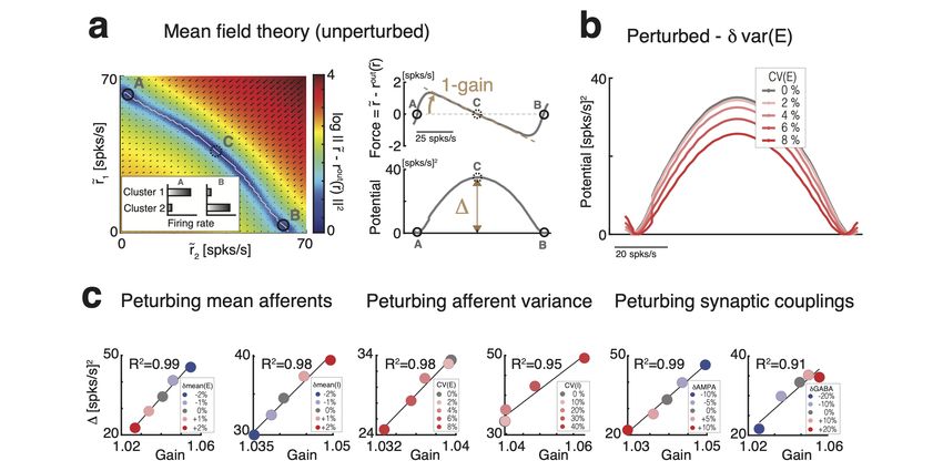
p−1
           "                                                                     !               #
         √                             + 2         − 2
                                                         X                   bgr
 σn2 = τm N nE pEE jEE
                    2
                                   f (JEE ) rn + (JEE ) (                                   2
                                                              rl + (1 − pf )rE )) − nI pEI jEI rI ,
                                                                    l=1
                                               p
                  "                                                            !                     #
 2
             √      2                − 2
                                               X                     bgr                     2
σbgr = τm N nE pEE jEE             (JEE )             rl + (1 − pf )rE             − nI pEI jEI rI       ,
                                                l=1
                                       p
                  "                                                 !                        #
             √                         X                      bgr
 σI = τm N                    2
                      nE pIE jIE   f         rl + (1 −   pf )rE         −            2
                                                                             nI pII jII rI       ,              (2.2)
                                       l=1

                                                                        bgr
where rn , rl = 1, . . . , p are the firing rates in the p E-clusters; rE   , rI , rext are the firing rates
in the background E population, in the I population, and in the external current. Other
parameters are described in Architecture and in Table 2. The network attractors satisfy
the self-consistent fixed point equations:

                                              rl = Fl [µl (r), σl2 (r)] ,                                      (2.3)

where r = (r1 , . . . , rp , rbgr , rI ) and l = 1, . . . , p, bgr, I, and Fl is the current-to-rate transfer
function for each population, which depend on the condition. In the absence of perturba-
tions, all populations have the LIF transfer function
                                                                Θl                 −1
                                                    √
                                                      Z
                                                                        u2
                         Fl (µl , σl ) = τref r + τm π               e [1 + erf(u)]    ,                       (2.4)
                                                               Hl

where Hl = (V reset − µl )/σl + ak and Θl = (Vlthr − µl )/σl + ak. k =           τs /τm and
                                                                               p
             √
a = |ζ(1/2)|/ 2 are terms accounting for the synaptic dynamics [33]. The perturbations
δvar(E) and δvar(I) induced an effective population transfer function F ef f on the E and I
populations, respectively, given by [20]:
                                         Z
                       Fα (µα , σα ) = DzFα (µα + zσz µext
                         pert                                   2
                                                           α , σα ) ,                  (2.5)
                                          √
where α = E, I and Dz = dz exp(−z 2 /2/ 2π) is a gaussian measure of zero mean and unit
                   √
variance, µext
            α = τm N nα pα0 jα0 rext is the external current and σz is the standard deviation
of the perturbation with respect to baseline, denoted CV(E) and CV(I). Stability of the
fixed point equation 2.3 was defined with respect to the approximate linearized dynamics
of the instantaneous mean ml and variance s2l of the input currents [20, 25]:

            dml                               ds2l
       τs       = −ml + µl (rl ) ;       τs        = −s2l + σl2 (rl ) ;          rl = Fl (ml (r), s2l (r)) ,   (2.6)
             dt                               2dt
where µl , σl2 are defined in 2.1-2.2 and Fl represents the appropriate transfer function 2.4
or 2.5. Fixed point stability required that the stability matrix

                            1 ∂Fl (µl , σl2 ) ∂Fl (µl , σl2 ) ∂σl2 (r)

                    Slm =                    −                         − δlm ,          (2.7)
                            τs      ∂rm           ∂σl2         ∂rm

was negative definite. The full mean field theory described above was used for the com-
prehensive analysis of Fig. 3-2.For the schematic of Fig. 3c, we replaced the LIF transfer

                                                         –7–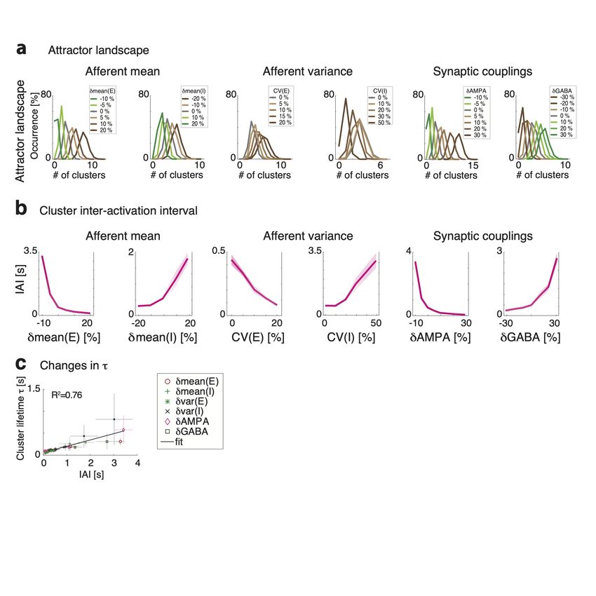
function 2.4 with the simpler function F̃ (µE ) = 0.5(1 + tanh(µE )) and the δvar(E) pertur-
bation effect was then modeled as F̃ ef f (µ) = Dz F̃ (µE + zσz µext ).
                                                                R

     Effective mean field theory for a reduced network. To calculate the potential energy
barrier separating the two network attractors in the reduced two-cluster network, we used
the effective mean field theory developed in [20, 34, 35]. The idea is to first estimate the
force acting on neural configurations with cluster firing rates r = [r̃1 , r̃2 ] outside the fixed
points (2.3), then project the two-dimensional system onto a one-dimensional trajectory
along which the force can be integrated to give an effective potential E (Fig. 3-2). In the
first step, we start from the full mean field equations for the P = p + 2 populations in 2.3,
and obtain an effective description of the dynamics for q populations “in focus” describing E
clusters (q = 2 in our case) by integrating out the remaining P − q out-of-focus populations
describing the background E neurons and the I neurons (P − q = 2 in our case). Given a
fixed value r̃ = [r̃1 , . . . , r̃q ] for the q in-focus populations, one obtains the stable fixed point
firing rates r0 = [rq+10     , . . . , rP0 ] of the out-of-focus populations by solving their mean field
equations
                                           rβ0 (r̃) = Fβ [µβ (r̃, r0 ), σβ2 (r̃, r0 )] ,           (2.8)
for β = q + 1, . . . , P , as function of the in-focus populations r̃, where stability is calculated
with respect to the condition (2.7) for the reduced (q + 1, . . . , P ) out-of-focus populations
at fixed values of the in-focus rates r̃. One then obtains a relation between the input r̃
and output values r̃out of the in-focus populations by inserting the fixed point rates of the
out-of-focus populations calculated in (2.8):

                             rαout (r̃) = Fα [µα (r̃, r0 (r̃)), σα2 (r̃, r0 (r̃))] ,              (2.9)

for α = 1, . . . , q. The original fixed points are r̃∗ such that r̃α∗ = rαout (r˜∗ ).
     Potential energy barriers and transfer function gain. In a reduced network with two
in-focus populations [r̃1 , r̃2 ] corresponding to the two E clusters, one can visualize Eq. (2.9)
as a two-dimensional force vector r̃ − rout (r̃) at each point in the two-dimensional firing rate
space r̃. The force vanishes at the stable fixed points A and B and at the unstable fixed
point C between them (Fig. 3-2). One can further reduce the system to one dimension by
approximating its dynamics along the trajectory between A and B as [34]:
                                              dr̃
                                         τs       = −r̃ + rout (r̃) ,                            (2.10)
                                              dt
where y = rout (r̃) represents an effective transfer function and r̃ − rout (r̃) an effective force.
                                                                               out     )−rout (r̃min )
We estimated the gain g of the effective transfer function as g = 1 − r (r̃r̃min    min −r̃max
                                                                                                       ,
where r̃min and r̃max represent, respectively, the minimum and maximum of the force (see
Fig. 3-2). From the one-dimensional dynamics (2.10) one can define a potential energy via
∂E(r̃)        out (r̃). The energy minima represent the stable fixed points A and B and the
  ∂r = r̃ − r
saddle point C between them represents the potential energy barrier separating the two
attractors. The height ∆ of the potential energy barrier is then given by
                                         Z C
                                   ∆=         dr̃[r̃ − rout (r̃)] ,                           (2.11)
                                                A

                                                     –8–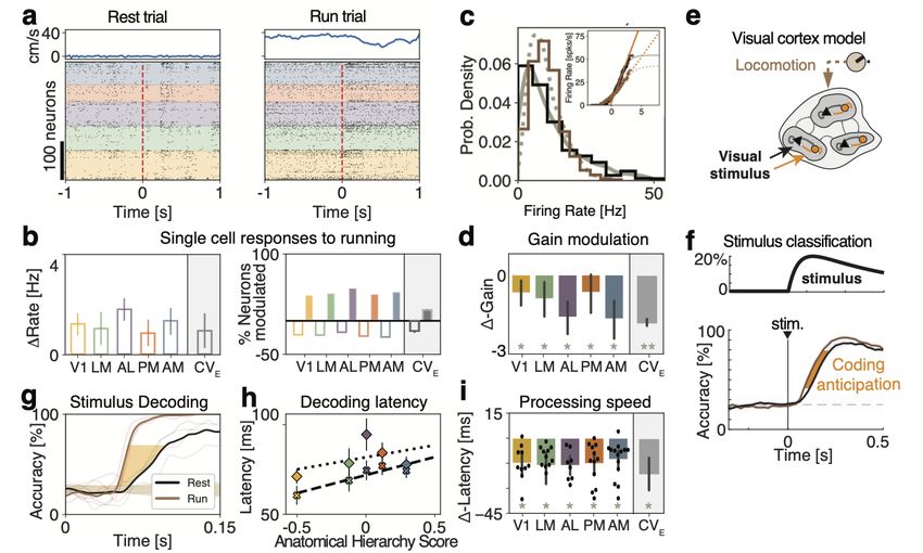
which can be visualized as the area of the curve between the effective transfer function and
the diagonal line (see Fig. 3).

2.3   Experimental data
We tested our model predictions using the open-source dataset of neuropixel recordings from
the Allen Institute for Brain Science [36]. We focused our analysis on experiments where
drifting gratings were presented at four directions (0◦ , 45◦ , 90◦ , 135◦ ) and one temporal
frequency (2 Hz). Out of the 54 sessions provided, only 7 sessions had enough trials per
behavioral condition to perform our decoding analysis. Neural activity from the visual
cortical hierarchy was collected and, specifically: primary visual cortex (V1) in 5 of these 7
sessions, with a median value of 75 neurons per session; lateral visual area (LM): 6 sessions,
47 neurons; anterolateral visual area (AL): 5 sessions, 61 neurons; posteromedial visual area
(PM): 6 sessions, 55; anteromedial visual area (AM): 7 sessions, 48 neurons. We matched
the number and duration of trials across condition and orientation and combined trials
from the drifting gratings repeat stimulus set, and drifting grating contrast stimulus set.
To do this, we combined trials with low-contrast gratings (0.08, 0.1, 0.13, 0.2; see Fig. 7-4)
and trials with high-contrast gratings (0.6, 0.8, 1; see Fig. 7-3) into separate trial types
to perform the decoding analysis, and analyzed the interval [−0.25, 0.5] seconds aligned to
stimulus onset.
     For evoked activity, running trials were classified as those where the animal was running
faster than 3 cm/s for the first 0.5 seconds of stimulus presentation. During ongoing activity,
behavioral periods were broken up into windows of 1 second. Periods of running or rest
were classified as such if 10 seconds had elapsed without a behavioral change. Blocks of
ongoing activity were sorted and used based on the length of the behavior. Out of the 54
sessions provided, 14 sessions had enough time per behavioral condition (minimum of 2
minutes) to estimate single-cell transfer functions. Only neurons with a mean firing rate
during ongoing activity greater than 5Hz were included in the gain analysis (2119 out of
4365 total neurons).

2.4   Stimulus decoding
For both the simulations and data, a multi-class decoder was trained to discriminate be-
tween four stimuli from single-trial population activity vectors in a given time bin [37]. To
create a timecourse of decoding accuracy, we used a sliding window of 100ms (200ms) in
the data (model), which was moved forward in 2ms (20ms) intervals in the data (model).
Trials were split into training and test data-sets in a stratified 5-fold cross-validated man-
ner, ensuring equal proportions of trials per orientation in both data-sets. In the model,
a leave-2-out cross-validation was performed. To calculate the significance of the decoding
accuracy, an iterative shuffle procedure was performed on each fold of the cross-validation.
On each shuffle, the training labels were shuffled and the classifer accuracy was predicted
on the unshuffled test data-set. This shuffle was performed 100 times to create a shuffle
distribution to rank the actual decoding accuracy from the unshuffled decoder against and
to determine when the mean decoding accuracy had increased above chance. This time
point is what we referred to as the latency of stimulus decoding. To account for the speed

                                            –9–
of stimulus decoding (the slope of the decoding curve), we defined the ∆-Latency between
running and rest as the average time between the two averaged decoding curves from 40%
up to 80% of the max decoding value at rest.
2.5 Firing rate distribution match
To control for increases of firing rate due to locomotion (Fig. 7b), we matched the distribu-
tions of population counts across the trials used for decoding in both behavioral conditions.
This procedure was done independently for each sliding window of time along the decoding
time course. Within each window, the spikes from all neurons were summed to get a pop-
ulation spike count per trial. A log-normal distribution was fit to the population counts
across trials for rest and running before the distribution match (Fig 7-1a left). We sorted
the distributions for rest and running in descending order, randomly removing spikes from
trials in the running distribution to match the corresponding trials in the rest distribution
(Fig 7-1a right). By doing this, we only removed the number of spikes necessary to match
the running distribution to rest distribution. For example, trials where the rest distribution
had a larger population count, no spikes were removed from either distribution. Given we
performed this procedure at the population level rather than per neuron, we checked the
change in PSTH between running and rest conditions before and after distribution matching
(Fig 7-1b). This procedure was also performed on the simulated data (Fig. 7-5).
2.6 Single-cell gain
To infer the single-cell transfer function in simulations and data, we followed the method
originally described in [38] (see also [39, 40] for a trial-averaged version). We estimated the
transfer function on ongoing periods when no sensory stimulus was present. Briefly, the
transfer function of a neuron was calculated by mapping the quantiles of a standard gaussian
distribution of input currents to the quantiles of the empirical firing rate distribution during
ongoing periods (Fig. 3d). We then fit this transfer function with a sigmoidal function.
The max firing rate of the neuron in the sigmoidal fit was bounded to be no larger than 1.5
times that of the empirical max firing rate, to ensure realistic fits. We defined the gain as
the slope at the inflection point of the sigmoid.
2.7 Single-cell response and selectivity
We estimated the proportion of neurons that were significantly excited or inhibited by
cortical state perturbations in the model (Fig. 6) or locomotion in the data (Fig. 7) during
periods of ongoing activity, in the absence of sensory stimuli. In the model, we simulated
40 trials per network, for 10 networks per each value of the perturbation; each trial in the
interval [−0.5, 1]s, with onset of the perturbation at t = 0 (the perturbation was modeled
as a double exponential with rise and decay times [0.2, 1], Fig. 3a). In the data, we binned
the spike counts in 500ms windows for each neuron after matching sample size between rest
and running conditions, and significant difference between the conditions was assessed with
a rank-sum test.
We estimated single neuron selectivity to sensory stimuli in each condition from the
average firing rate responses ria (t) of the i-th neuron to stimulus a in trial t. For each pair
– 10 –Figure 1. Conceptual summary of the main results. a): In a network model of sensory cortex
featuring clusters of excitatory and inhibitory neurons with metastable dynamics, state changes
are induced by external perturbations controlling the timescale of cluster activation during ongoing
activity. The neural mechanism underlying timescale modulation is a change in the barrier height
separating attractors, driven by a modulation of the intrinsic gain of the single-cell transfer function.
b): During evoked activity, onset of stimulus encoding is determined by the activation latency
of stimulus-selective cluster. External perturbations modulate the onset latency thus controlling
the stimulus processing speed. The theory shows that the effect of external perturbations on
stimulus-processing speed during evoked activity (right) can be predicted by the induced gain
modulations observed during ongoing activity (left). c): Locomotion induced changes in intrinsic
gain in the visual cortical hierarchy during darkness periods. d): Locomotion drove faster coding of
visual stimuli during evoked periods, as predicted by the induced gain modulations observed during
ongoing activity.
of stimuli, selectivity was estimated as
mean a ] − mean r(t)b
[r(t)
d0 (a, b) = q ,
1
(var[r(t) a ] + var[r(t)b ])
2
where mean and var are estimated across trials. The d’ was then averaged across stimulus
pairs.
– 11 –Figure 2. Biological plausible model of cortical circuit. a) Schematics of the network architecture.
A recurrent network of E (black triangles) and I (red circles) spiking neurons arranged in clusters is
presented sensory stimuli targeting subsets of E clusters, in different cortical states implemented by
perturbations. Inset shows a membrane potential trace from representative E neuron. b) Synaptic
couplings Jij for a representative clustered network, highlighting the block diagonal structure of
potentiated intra-cluster synaptic weights for both E and I clusters, and the background E and I
populations (bgr). Cluster size was heterogeneous (inset). c) Representative neural activity during
ongoing periods; tick marks represent spike times of E (black) or I (red) neurons. The network
dynamics is metastable with clusters transiently activity for periods of duration τ . Inset: The
cumulative distributions of single-cell firing rates (in the representative network are lognormal (blue:
empirical data; orange: lognormal fit). c) Left: State-changing perturbation affecting the mean of
the afferent currents to E populations (knobs represent changes in afferent to three representative
E cells compared to the unperturbed state). Right: Histogram of afferent inputs to E-cells in the
perturbed state (brown, all neurons receive a 10% increase in input) with respect to the unperturbed
state (grey). d) Left: State-changing perturbation affecting the variance of afferent currents to E
populations. Right: In the perturbed state (brown), each E-cell’s afferent input is constant and
sampled from a normal distribution with mean equal to the unperturbed value (grey) and 10% CV.
3 Results
To elucidate the effect of state changes on cortical dynamics, we modeled the local circuit as
a network of recurrently connected excitatory (E) and inhibitory (I) spiking neurons. Both
E and I populations were arranged in clusters [20, 22, 23, 25, 41], where synaptic couplings
– 12 –between neurons in the same cluster were potentiated compared to neurons in different
clusters, reflecting the empirical observation of cortical assemblies of functionally correlated
neurons [Fig. 2a; 42–45]. In the absence of external stimulation (ongoing activity), this E-I
clustered network generates rich temporal dynamics characterized by metastable activity
operating in inhibition stabilized regime, where E and I post-synaptic currents track each
other achieving tight balance (Fig. 2-1). A heterogeneous distribution of cluster sizes leads
to a lognormal distributions of firing rates (Fig. 2b). Network activity was characterized by
the emergence of the slow timescale of cluster transient activation, with average activation
lifetime of τ = 106 ± 35 ms (hereby referred to as “cluster timescale," Fig. 2b), much larger
than single neuron time constant [20ms; 23, 25].
To investigate how changes in cortical state may affect the network dynamics and infor-
mation processing capabilities, we examined a vast range of state-changing perturbations
(Fig. 2c-d, Table 3). State changes were implemented as perturbations of the afferent
currents to cell-type specific populations, or as perturbations to the synaptic couplings.
The first type of state perturbations δmean(E) affected the mean of the afferent currents
to E populations (Fig. 2c). E.g., a perturbation δmean(E)=10% implemented an increase
of all input currents to E neurons by 10% above their unperturbed levels. The perturba-
tion δmean(I) affected the mean of the afferent currents to I populations in an analogous
way. The second type of state perturbations δvar(E) affected the across-neuron variance
of afferents to E populations. Namely, in this perturbed state, the afferent current to each
neuron in that population was sampled from a normal distribution with zero mean and fixed
variance (Fig. 2d, measured by the coefficient of variability CV(E)=var(E)/mean(E) with
respect to the unperturbed afferents). This perturbation thus introduced a spatial variance
across neurons in the cell-type specific afferent currents, yet left the mean afferent current
into the population unchanged. The state perturbation δvar(I) affected the variance of
the afferent currents to I populations analogously. In the third type of state perturbations
δAMPA or δGABA, we changed the average GABAergic or glutamatergic (AMPA) recur-
rent synaptic weights compared to their unperturbed values. We chose the range of state
perturbations such that the network still retained non-trivial metastable dynamics within
the whole range. We will refer to these state changes of the network as simply perturbations,
and should not be confused with the presentation of the stimulus. We first established the
effects of perturbations on ongoing network dynamics, and used those insight to explain
their effects on stimulus-evoked activity.
3.1 State-dependent regulation of the network emergent timescale
A crucial feature of neural activity in clustered networks is metastable attractor dy-
namics, characterized by the emergence of a long timescale of cluster activation whereby
network itinerant activity explores the large attractor landscape (Fig. 2b). We first exam-
ined whether perturbations modulated the network’s metastable dynamics and introduced
a protocol where perturbations occurred in the absence of sensory stimuli (“ongoing activ-
ity”).
We found that perturbations strongly modulated the attractor landscape, changing
the repertoire of attractors the network activity visited during its itinerant dynamics (Fig.
– 13 –3a and 3-1a). Changes in attractor landscape were perturbation-specific. Perturbations
increasing δmean(E) (δmean(I)) induced a consistent shift in the repertoire of attractors:
larger perturbations led to larger (smaller) numbers of co-active clusters. Surprisingly,
perturbations that increased δvar(E) (δvar(I)), led to network configurations with larger
(smaller) sets of co-activated clusters. This effect occurred despite the fact that such per-
turbations did not change the mean afferent input to the network. Perturbations affecting
δAMPA and δGABA had similar effects to δmean(E) and δmean(I), respectively.
We then examined whether perturbations affected the cluster activation timescale. We
found that perturbations differentially modulated the average cluster activation timescale
τ during ongoing periods, in the absence of stimuli (Fig. 3b). In particular, increasing
δmean(E), δvar(E), or δAMPA led to a proportional acceleration of the network metastable
activity and shorter τ ; while increasing δmean(I), δvar(I) or δGABA induced the opposite
effect with longer τ . Changes in τ were congruent with changes in the duration of intervals
between consecutive activations of the same cluster (cluster inter-activation intervals, Fig.
3-1).
3.2 Changes in cluster timescale are controlled by gain modulation
What is the computational mechanism mediating the changes in cluster timescale, induced
by the perturbations? We investigated this question using mean field theory, where network
attractors, defined by sets of co-activated clusters, are represented as potential wells in an
attractor landscape [20, 23, 25, 34, 46]. Let us illustrate this in a simplified network with
two clusters (Fig. 3c and 3-2). Here, the attractor landscape consists of two potential
wells, each well corresponding to a configuration where one cluster is active and the other is
inactive. When the network activity dwells in the attractor represented by the left potential
well, it may escape to the right potential well due to internally generated variability. This
process will occur with a probability determined by the height ∆ of the barrier separating
the two wells: the higher the barrier, the less likely the transition [20, 23, 46, 47]. Mean
field theory thus established a relationship between the cluster timescale and the height of
the barrier separating the two attractors. We found that perturbations differentially control
the height of the barrier ∆ separating the two attractors (Fig. 3-2), explaining the changes
in cluster timescale observed in the simulations (Fig. 3b).
Since reconstruction of the attractor landscape requires knowledge of the network’s
structural connectivity, the direct test of the mean field relation between changes in at-
tractor landscape and timescale modulations is challenging. We thus aimed at obtaining
an alternative formulation of the underlying neural mechanism only involving quantities
directly accessible to experimental observation. Using mean field theory, one can show that
the double potential well representing the two attractors can be directly mapped to the
effective transfer function of a neural population [20, 34, 35]. One can thus establish a di-
rect relationship between changes in the slope (hereby referred to as “gain") of the intrinsic
transfer function estimated during ongoing periods and changes in the barrier height ∆
separating metastable attractors (see Fig. 3c, 3-2 and Methods). In turn, this implies a
direct relationship between gain modulation, induced by the perturbations, and changes in
cluster activation timescale. In particular, perturbations inducing steeper gain will increase
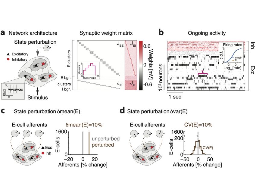
– 14 –Figure 3. Linking gain modulation to changes in cluster timescale. a) Top left: Clustered net-
work activity during a representative ongoing trial hops among different metastable attractors (grey
box: attractor with 3 co-active clusters). Bottom: Number of co-active clusters at each time bin
(right: frequency of occurrence of attractors with 2-6 co-active clusters in the representative trial).
Right: Perturbations strongly modulate the attractor landscape (color-coded curves: frequency of
occurrence of network attractors with different number of co-active clusters, for different values of
the representative δmean(E) perturbation, mean occurrence across 5 sessions). b) Perturbations
induce consistent changes in the average cluster activation timescale τ (mean±S.D. across 5 sim-
ulated sessions) and in the single neuron intrinsic gain (estimated as in panel d). c) Schematic of
the effect of perturbations on network dynamics. Dynamics in a two-cluster network is captured
by its effective potential energy (top panel). Potential wells represent two attractors where either
cluster is active (A and B). Perturbations that shrink the barrier height ∆ separating the attractors
induce faster transition rates between attractors and shorter cluster activation lifetime (black and
brown: unperturbed and perturbed conditions, respectively).
– 15 –well depths and barrier heights, and thus increase the cluster timescale, and vice versa.
Using mean field theory, we demonstrated a complete classification of the differential effect
of all perturbations on barrier heights and gain (Fig. 3-2).
We then proceeded to verify these theoretical predictions, obtained in a simplified two-
cluster network, in the high dimensional case of large networks with several clusters using
simulations. While barrier heights and the network’s attractor landscape can be exactly
calculated in the simplified two-cluster network, this task is infeasible in large networks with
a large number of clusters where the number of attractors is exponential in the number of
clusters. On the other hand, changes in barrier heights ∆ are equivalent to changes in gain,
and the latter can be easily estimated from spiking activity (Fig. 3b and 3-2). We thus
tested whether the relation between gain and timescale held in the high-dimensional case of
a network with many clusters. We estimated single-cell transfer functions from their spiking
activity during ongoing periods, in the absence of sensory stimuli but in the presence of
different perturbations (Fig. 3d, [38, 39]). We found that network perturbations strongly
modulated single-cell gain in the absence of stimuli, verifying mean field theory predictions
in all cases (Fig. 3d). In particular, we confirmed the direct relationship between gain
modulation and cluster timescale modulation: perturbations that decreased (increased) the
gain also decreased (increased) cluster timescale (Fig. 3e, R2 = 0.96). For all perturbations,
gain modulations explained the observed changes in cluster timescale.
3.3 Controlling information processing speed with perturbations
We found that changes in cortical state during ongoing activity, driven by external pertur-
bations, control the circuit’s dynamical timescale. The neural mechanism mediating the
effects of external perturbations is gain modulation, which controls the timescale of the
network switching dynamics. How do such state changes affect the network information
processing speed?
To investigate the effect of state perturbations on the network’s information-processing,
we compared stimulus-evoked activity by presenting stimuli in an unperturbed and a per-
turbed condition. In unperturbed trials (Fig. 4a), we presented one of four sensory stimuli,
modeled as depolarizing currents targeting a subset of stimulus-selective E neurons with
linearly ramping time course. Stimulus selectivities were mixed and random, all clusters
having equal probability of being stimulus-selective. In perturbed trials (Fig. 4b), in ad-
dition to the same sensory stimuli, we included a state perturbation, which was turned on
before the stimulus and was active until the end of stimulus presentation. We investigated
Legend continued : Mean field theory provides a relation between potential energy and transfer
function (bottom panel), thus linking cluster lifetime to neuronal gain in the absence of stimuli
(dashed blue line, gain). d): A single-cell transfer function (bottom, empirical data in blue; sig-
moidal fit in brown) can be estimated by matching a neuron’s firing rate distribution during ongoing
periods (top) to a gaussian distribution of input currents (center, quantile plots; red stars denotes
matched median values). e) Perturbation-induced changes in gain (x-axis: gain change in perturbed
minus unperturbed condition, mean±s.e.m. across 10 networks; color-coded markers represent dif-
ferent perturbations) explain changes in cluster lifetime (y-axis, linear regression, R2 = 0.96) as
predicted by mean field theory (same as in panel b).
– 16 –and classified the effect of several state changes implemented by perturbations affecting
either the mean or variance of cell-type specific afferents to E or I populations, and the
synaptic couplings. State perturbations were identical in all trials of the perturbed condi-
tion for each type; namely, they did not convey any information about the stimuli.
We assessed how much information about the stimuli was encoded in the population
spike trains at each moment using a multiclass classifier (with four class labels correspond-
ing to the four presented stimuli, Fig. 4c). In the unperturbed condition, the time course
of the cross-validated decoding accuracy, averaged across stimuli, was significantly above
chance after 0.21 + / − 0.02 seconds (mean±s.e.m. across 10 simulated networks, black
curve in Fig. 4c) and reached perfect accuracy after a second. In the perturbed condition,
stimulus identity was decoded at chance level in the period after the onset of the state per-
turbation but before stimulus presentation (Fig. 4c), consistent with the fact that the state
perturbation did not convey information about the stimuli. We found that state pertur-
bations significantly modulated the network information processing speed. We quantified
this modulation as the average latency to reach a decoding accuracy between 40% and 80%
(Fig. 4c, yellow area), and found that state perturbations differentially affected processing
speed.
State perturbations had opposite effects depending on which cell-type specific popula-
tions they targeted. Increasing δmean(E) monotonically improved network performance
(Fig. 4d, left panel): in particular, positive perturbations induced an anticipation of
stimulus-coding (shorter latency), while negative ones led to longer latency and slower
coding. The opposite effect was achieved when increasing δmean(I), which slowed down
processing speed (Fig. 4d, right panel). State perturbations that changed the spatial
variance of the afferent currents had counterintuitive effects (Fig. 4e). We measured the
strength of these perturbations via their coefficient of variability CV (α) = σα /µα , for
α = E, I, where σ and µ are the standard deviation and mean of the across-neuron dis-
tribution of afferent currents. Perturbations δvar(E) that increased CV (E) led to faster
processing speed. The opposite effect was achieved with perturbations δvar(I) inducing a
spatial variance across afferents to I neurons, which slowed down stimulus-processing speed
(Fig. 4e). Perturbations δAMPA which increased the glutamatergic synaptic weights im-
proved performance proportionally to the perturbation. The opposite effect was achieved
by perturbations δGABA that increased the GABAergic synaptic weights, which mono-
tonically decreased network processing speed (Fig. 4f). We thus concluded that afferent
current perturbations differentially modulated the speed at which network activity encoded
information about incoming sensory inputs. Such modulations exhibited a rich dynamical
repertoire (Table 3).
3.4 Gain modulation regulates the network information processing speed
Our mean field framework demonstrates a direct relationship between the effects of
perturbations on the network information processing speed and its effects on the cluster
timescale (Fig. 3). In our simplified network with two clusters, stimulus presentation
induces an asymmetry in the well depths, where the attractor B corresponding to the
activated stimulus-selective cluster has a deeper well, compared to the attractor A where
– 17 –Figure 4. Perturbations control stimulus-processing speed in the clustered network. a-b) Represen-
tative trials in the unperturbed (a) and perturbed (b) conditions; the representative perturbation is
an increase in the spatial variance δvar(E) across E neurons. After a ramping stimulus is presented
at t = 0 (black vertical line on raster plot; top panel, stimulus time course), stimulus-selective
E-clusters (brown tick marks represent their spiking activity) are activated at a certain latency
(brown vertical line). In the perturbed condition (b), a perturbation is turned on before stimulus
onset (gray-dashed vertical line). The activation latency of stimulus-selective clusters is shorter in
the perturbed compared to the unperturbed condition. c) Left: schematic of stimulus-decoding
analysis. A multi-class classifier is trained to discriminate between the four stimuli from single-trial
population activity vectors in a given time bin (curves represent the time course of population
activity in single trials, color-coded for 4 stimuli; the purple circle highlights a given time bin along
the trajectories), yielding a cross-validated confusion matrix for the decoding accuracy at that bin
(central panel). Right: Average time course of the stimulus-decoding accuracy in the unperturbed
(black) and perturbed (brown) conditions (horizontal brown: significant difference between condi-
tions, p < 0.05 with multiple bin correction). d-f: Difference in stimulus decoding latency in the
perturbed minus the unperturbed conditions (average difference between decoding accuracy time
courses in the [40%,80%] range, yellow interval of c; mean±S.D. across 10 networks) for the six
state-changing perturbations (see Methods and main text for details; the brown star represents the
perturbation in b-c).
the stimulus-selective cluster is inactive. Upon stimulus presentation, the network ongoing
state will be biased to transition towards the stimulus-selective attractor B with a transition
rate determined by the barrier height separating A to B. Because external perturbations
regulate the height of such barrier via gain modulation, they control in turn the latency
of activation of the stimulus-selective cluster. We thus aimed at testing the prediction
of our theory: that the perturbations modulate stimulus coding latency in the same way
as they modulate cluster timescales during ongoing periods; and, as a consequence, that
these changes in stimulus coding latency can be predicted by intrinsic gain modulation.
– 18 –Latency Activity Response τ Gain
δmean(E)% & E[%], I[%] E[%], I[%] & &
δmean(I)% % E[&], I[&] E[&], I[mixed] % %
δvar(E)% & E[%], I[%] E[mixed], I[mixed] & &
δvar(I)% % E[&], I[=] E[&], I[&] % %
δAMPA% & E[%], I[%] E[%], I[%] & &
δGABA% % E[&], I[&] E[&], I[mixed] % %
Locomotion & E[%], I[%] E[mixed], I[mixed] & &
Table 3. Classification of state-changing perturbations. Effect of on neural activity of an increasing
(%) state-changing perturbation: latency of stimulus decoding (’Latency’, Fig. 2d); average firing
rate modulation (’Activity’) and response to perturbations (’Response’, proportion of cells with
significant responses) of E and I cells in the absence of stimuli (Fig. 3); cluster activation timescale
(’τ ’, Fig. 4b); single-cell intrinsic gain modulation at rest (’Gain’, Fig. 5e). %, &, = represent
increase, decrease, and no change, respectively. ’Mixed’ responses refer to similar proportions of
excited and inhibited cells. The effect of locomotion is consistent with a perturbation increasing
δvar(E).
Specifically, our theory predicts that perturbation driving a decrease (increase) in intrinsic
gain during ongoing periods will induce a faster (slower) encoding of the stimulus.
We thus proceeded to test the relationship between perturbations effects on cluster
timescales, gain modulation, and information processing speed. In the representative trial
where the same stimulus was presented in the absence (Fig. 4a) or in the presence (Fig. 4b)
of the perturbation δmean(E)= 10%, we found that stimulus-selective clusters (highlighted
in brown) had a faster activation latency in response to the stimulus in the perturbed con-
dition compared to the unperturbed one. A systematic analysis confirmed this mechanism
showing that, for all perturbations, the activation latency of stimulus-selective clusters was
a strong predictor of the change in decoding latency (Fig. 5a right panel, R2 = 0.93).
Moreover, we found that the perturbation-induced changes of the cluster timescale τ dur-
ing ongoing periods predicted the effect of the perturbation on stimulus-processing latency
during evoked periods (Fig. 5b,d). Specifically, perturbations inducing faster τ during on-
going periods, in turn accelerated stimulus coding; and vice versa for perturbations inducing
slower τ .
We then tested whether perturbation-induced gain modulations during ongoing periods
explained the changes in stimulus-processing speed during evoked periods, and found that
the theoretical prediction was borne out in the simulations (Fig. 5c,e). Let us summarize
the conclusion of our theoretical analyses. Motivated by mean field theory linking gain
modulation to changes in transition rates between attractors, we found that gain modulation
controls the cluster timescale during ongoing periods, and, in turn, regulates the onset
latency of stimulus-selective clusters upon stimulus presentation. Changes in onset latency
of stimulus-selective clusters explained changes in stimulus-coding latency. We thus linked
– 19 –You can also read