Incorporating the stable carbon isotope 13C in the ocean biogeochemical component of the Max Planck Institute Earth System Model - Biogeosciences
←
→
Page content transcription
If your browser does not render page correctly, please read the page content below
Biogeosciences, 18, 4389–4429, 2021
https://doi.org/10.5194/bg-18-4389-2021
© Author(s) 2021. This work is distributed under
the Creative Commons Attribution 4.0 License.

Incorporating the stable carbon isotope 13C in the ocean
biogeochemical component of the Max Planck Institute
Earth System Model
Bo Liu, Katharina D. Six, and Tatiana Ilyina
Ocean in the Earth System, Max Planck Institute for Meteorology, Hamburg, Germany

Correspondence: Bo Liu (bo.liu@mpimet.mpg.de)

Received: 9 February 2021 – Discussion started: 12 February 2021
Revised: 27 May 2021 – Accepted: 4 June 2021 – Published: 28 July 2021

Abstract. The stable carbon isotopic composition (δ 13 C) is         underestimation, but their approach does not provide any in-
an important variable to study the ocean carbon cycle across         sight about the cause. By applying the Eide et al. (2017a)
different timescales. We include a new representation of the         approach to the model data we are able to investigate in de-
stable carbon isotope 13 C into the HAMburg Ocean Car-               tail potential sources of underestimation of the 13 C Suess ef-
bon Cycle model (HAMOCC), the ocean biogeochemical                   fect. Based on our model we find underestimations of the 13 C
component of the Max Planck Institute Earth System Model             Suess effect at 200 m by 0.24 ‰ in the Indian Ocean, 0.21 ‰
(MPI-ESM). 13 C is explicitly resolved for all oceanic carbon        in the North Pacific, 0.26 ‰ in the South Pacific, 0.1 ‰ in the
pools considered. We account for fractionation during air–           North Atlantic and 0.14 ‰ in the South Atlantic. We attribute
sea gas exchange and for biological fractionation p associ-         the major sources of underestimation to two assumptions in
ated with photosynthetic carbon fixation during phytoplank-          the Eide et al. (2017a) approach: the spatially uniform pre-
ton growth. We examine two p parameterisations of dif-              formed component of δ 13 CDIC in year 1940 and the neglect
                       Popp                                          of processes that are not directly linked to the oceanic uptake
ferent complexity: p        varies with surface dissolved CO2
concentration (Popp et al., 1989), while pLaws additionally         and transport of chlorofluorocarbon-12 (CFC-12) such as the
depends on local phytoplankton growth rates (Laws et al.,            decrease in δ 13 CPOC over the industrial period.
1995). When compared to observations of δ 13 C of dissolved             The new 13 C module in the ocean biogeochemical com-
inorganic carbon (DIC), both parameterisations yield simi-           ponent of MPI-ESM shows satisfying performance. It is a
lar performance. However, with regard to δ 13 C in particulate       useful tool to study the ocean carbon sink under the anthro-
                           Popp                                      pogenic influences, and it will be applied to investigating
organic carbon (POC) p          shows a considerably improved
performance compared to pLaws . This is because pLaws pro-         variations of ocean carbon cycle in the past.
duces too strong a preference for 12 C, resulting in δ 13 CPOC
that is too low in our model. The model also well reproduces
the global oceanic anthropogenic CO2 sink and the oceanic
13 C Suess effect, i.e. the intrusion and distribution of the iso-   1   Introduction
topically light anthropogenic CO2 in the ocean.
                                                                     The stable carbon isotopic composition (δ 13 C) measured
   The satisfactory model performance of the present-day
                                       Popp                          in carbonate shells of fossil foraminifera is one of the
oceanic δ 13 C distribution using p         and of the anthro-
                                                                     most widely used properties in paleoceanographic re-
pogenic CO2 uptake allows us to further investigate the po-
                                                                     search (Schmittner et al., 2017). It is defined as a normalised
tential sources of uncertainty of the Eide et al. (2017a) ap-
                                                                     ratio between the stable carbon isotopes 13 C and 12 C:
proach for estimating the oceanic 13 C Suess effect. Eide et al.
(2017a) derived the first global oceanic 13 C Suess effect es-                      13
                                                                                          C/12 C

timate based on observations. They have noted a potential            δ 13 C(‰) =                 − 1 · 1000,                    (1)
                                                                                          Rstd

Published by Copernicus Publications on behalf of the European Geosciences Union.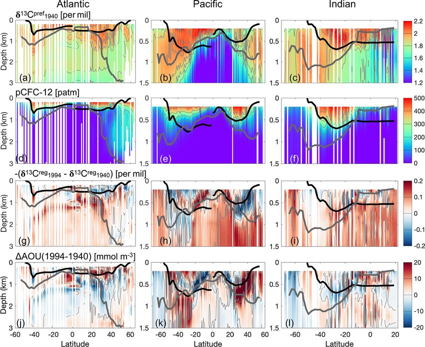
4390                                                                                    B. Liu et al.: 13 C module in MPI-ESM

where Rstd is an arbitrary standard ratio. In observational        size and shape (e.g. Rau et al., 1996; Keller and Morel, 1999),
studies, the ratio 13 C/12 C in Pee Dee Belemnite (PDB;            as HAMOCC6 does not resolve these features of plankton
Craig, 1957) is conventionally used for Rstd .                     cells.
   δ 13 C provides information on past changes in water mass          Oceanic δ 13 C measurements were mostly carried out in
distribution and properties (e.g. Curry and Oppo, 2005; Pe-        the late 20th century. In the upper ocean δ 13 C in dissolved
terson et al., 2014). Direct comparison between paleo-δ 13 C       inorganic carbon (δ 13 CDIC ) has been observed to notice-
measurements and simulated δ 13 C facilitates evaluating the       ably decrease in response to the intrusion of anthropogenic
ability of Earth system models (ESMs) to simulate paleo-           CO2 from fossil fuel combustion which carries a lower
ocean states. For this reason, we present a new implemen-          13 C/12 C signal (Gruber et al., 1999; Quay et al., 2003). Such

tation of 13 C in the HAMburg Ocean Carbon Cycle model             δ 13 CDIC decrease is referred to as the oceanic 13 C Suess ef-
(HAMOCC6), the ocean biogeochemical component of the               fect (Keeling, 1979). Recently, Eide et al. (2017a) derived an
Max Planck Institute Earth System Model (MPI-ESM). A               observation-based estimate of the global ocean 13 C Suess ef-
comprehensive representation of δ 13 C is a timely extension       fect since pre-industrial times. Such an observation-based es-
of MPI-ESM in support of planned simulations of a complete         timate is valuable as it is the basis of an almost independent
last glacial cycle within the German climate modelling initia-     estimate of the global ocean anthropogenic carbon uptake.
tive PalMod (Latif et al., 2016). Before applying the new 13 C     And it could be used for evaluating models at pre-industrial
module to paleo-simulations, we evaluate it by comparison          states (Buchanan et al., 2019; Tjiputra et al., 2020) and for
to observational data in the present-day ocean.                    setting up paleo-simulations (O’Neill et al., 2019).
   Earlier versions of HAMOCC already featured a 13 C mod-            Yet, Eide et al. (2017a) have noted that their approach
ule, for instance HAMOCC2s (Heinze and Maier-Reimer,               might underestimate the oceanic 13 C Suess effect. They con-
1999) and HAMOCC3 (Maier-Reimer, 1993). HAMOCC3                    jectured an underestimation of the 13 C Suess effect between
included prognostic 13 C variables for dissolved inorganic         0.15 ‰–0.24 ‰ at 200 m depth in 1994. However, the quan-
carbon (DIC), particulate organic matter and calcium carbon-       titative spatial distribution of this underestimation is unclear.
ate. HAMOCC3 also accounted for temperature-dependent              Moreover, although Eide et al. (2017a) have related the un-
isotopic fractionation during air–sea gas exchange (higher         derestimation to several assumptions in the approach they ap-
δ 13 C of surface DIC in colder water) and biological frac-        plied, the quantitative impact of these assumptions is still un-
tionation during carbon fixation. Due to the simplified rep-       clear as the measurements are too limited in space and time
resentation of marine biological production in HAMOCC3,            to perform in-depth investigation.
biological fractionation was based on fixation of inorganic           Our model data include all parameters needed to apply
carbon into non-living particulate organic matter and was          the Eide et al. (2017a) procedure, which relies on regres-
parameterised by a spatially and temporally uniform factor.        sional relationships between preformed δ 13 CDIC (related to
This approach for biological fractionation of 13 C, however,       the transport of surface waters with specific DIC and DI13 C)
could not reproduce the observed large meridional gradi-           and CFC-12 (chlorofluorocarbon-12) partial pressure. Thus,
ent of δ 13 C in particulate organic matter (Goericke and Fry,     our consistent model framework, with the complete spatio-
1994). Since then, HAMOCC3 was refined in particular with          temporal information of the hydrological and biogeochem-
regard to its representation of plankton dynamics. The cur-        ical variables, enables us to investigate the spatial distribu-
rent version HAMOCC6 resolves bulk phytoplankton, zoo-             tion of the above-mentioned potential underestimation of the
plankton, detritus, dissolved organic carbon (Six and Maier-       oceanic 13 C Suess effect. Moreover, our model framework
Reimer, 1996) and nitrogen-fixing cyanobacteria (Paulsen           also allows for the attribution of the underestimation to the
et al., 2017). We thus develop an updated 13 C module that         assumptions of the procedure Eide et al. (2017a) applied.
considers the refined ecosystem representation and test dif-          In the following sections, we first provide a brief introduc-
ferent non-uniform parameterisations for biological fraction-      tion to the global ocean biogeochemical model HAMOCC6,
ation during phytoplankton growth.                                 followed by a description of the new 13 C module including
   To choose a suitable biological fractionation parameteri-       the experimental setup (Sect. 2). Section 3 presents the model
sation for our model, we test the parameterisations of Popp        evaluation against observations in the late 20th century, and
et al. (1989) and Laws et al. (1995). These parameterisa-          Sect. 4 evaluates the simulated oceanic 13 C Suess effect. Sec-
tions are selected for two reasons. First, they are of different   tion 5 addresses our findings on testing the Eide et al. (2017a)
complexities. The parameterisation of Popp et al. (1989) em-       approach for estimating the oceanic 13 C Suess effect. Sum-
pirically relates 13 C biological fractionation to the concen-     mary and conclusions are given in Sect. 6.
tration of dissolved CO2 in seawater, whereas that of Laws
et al. (1995) considers dissolved CO2 concentration and phy-
toplankton growth rate. Second, input variables in these two
parameterisations are explicitly computed in the model. We
omit more complex parameterisations that include effects of
cell membrane permeability of molecular CO2 diffusion, cell

Biogeosciences, 18, 4389–4429, 2021                                                   https://doi.org/10.5194/bg-18-4389-2021
B. Liu et al.: 13 C module in MPI-ESM                                                                                        4391

2     Model description                                            assume 12 C = C. We include a 13 C counterpart for each 12 C
                                                                   prognostic variable; that is, we introduce seven new tracers
2.1    The global ocean biogeochemical model                       for the water column and three for the sediment. 13 C only
       (HAMOCC6)                                                   mimics the 12 C biogeochemical fluxes, modified by the cor-
                                                                   responding isotopic fractionation. We assume 13 C inventory
HAMOCC6 (Ilyina et al., 2013; Paulsen et al., 2017; Mau-           to be as large as the inventory of 12 C to reduce numerical er-
ritsen et al., 2019) includes biogeochemical processes in          rors. Consequently, the reference standard of the stable car-
the water column and in the sediment. In the water col-            bon isotope ratio Rstd is set to 1 in Eq. (1). In this section,
umn, the following biogeochemical tracers are simulated:           we describe the implementation of 13 C fractionation during
dissolved inorganic carbon (DIC), total alkalinity (TA),           air–sea exchange and carbon uptake by bulk phytoplankton
phosphate (PO4 ), nitrate (NO3 ), nitrous oxide (N2 O), dis-       and by cyanobacteria. Because the isotopic fractionation dur-
solved nitrogen gas (N2 ), silicate (SiO4 ), dissolved bioavail-   ing the production of calcium carbonate is small (Turner,
able iron (Fe), dissolved oxygen (O2 ), bulk phytoplankton         1982) and uncertain (Zeebe and Wolf-Gladrow, 2001), it is
(Phy), cyanobacteria (Cya), zooplankton (Zoo), dissolved or-       not considered in this study, following the model studies of
ganic matter (DOM), particulate organic matter (POM), opal         e.g. Lynch-Stieglitz et al. (1995), Schmittner et al. (2013) and
shells, calcium carbonate shells (CaCO3 ), terrigenous mate-       Tjiputra et al. (2020).
rial (Dust) and hydrogen sulfide (H2 S). Below the model-
defined export depth (100 m), the sinking speed of POM             2.2.1     Fractionation during air–sea gas exchange
linearly increases with depth. Theoretically, this leads to
a power-law-like attenuation of POM fluxes as observa-             The net air–sea CO2 gas exchange flux F reads

tions (Martin et al., 1987; Kriest and Oschlies, 2008). Con-       F = −kCO2 γCO2 pCO2 surf − pCO2 atm .                       (2)
stant sinking speeds are set for opal, CaCO3 and Dust. Except
for CaCO3 and opal, whose sinking speeds (30 and 25 m d−1 ,        Here, pCO2 surf and pCO2 atm are the partial pressures of CO2
respectively) are considerably faster than the horizontal ve-      in the surface seawater and in the atmosphere, respectively.
locities of ocean flow, the water-column biogeochemical            The piston velocity kCO2 (m s−1 ) for CO2 and the solubility
tracers are transported by the hydrodynamical fields in the        γCO2 (mol L−1 atm−1 ) of CO2 are calculated following Wan-
same manner as salinity.                                           ninkhof (2014) and Weiss (1974), respectively.
   The sediment module is based on Heinze et al. (1999).              Similar to the air–sea flux of total carbon in Eq. (2), the
It simulates remineralisation and dissolution processes as in      net air–sea 13 CO2 exchange flux 13 F reads
the water column concerning dissolved tracers (PO4 , NO3 ,
                                                                   13
N2 , O2 , SiO4 , Fe, H2 S, DIC and TA) in the pore water and          F = −13 kCO2 13 γCO2 pCO2 surf Rg − pCO2 atm Ratm , (3)
the solid sediment constituents (POM, opal, CaCO3 ). The
tracers in the pore water are exchanged with the overlying         in which Rg and Ratm are the ratios of 13 C/12 C in sur-
water column by diffusion. Pelagic sedimentation fluxes of         face pCO2 and in atmospheric CO2 , respectively. Following
POM, CaCO3 and opal are added to the solid components of           Zhang et al. (1995), we can rewrite Eq. (3) as
the sediment. Below the active sediment there is one layer         13
                                                                        F = −kCO2 αk γCO2 αaq←g
containing only solid sediment components and representing
burial. To balance the loss of nutrients, TA, DIC and SiO4 in                          RDIC
                                                                            pCO2 surf        − pCO2 atm Ratm .                 (4)
the water column, constant input fluxes of DOM, CO2−     3 and
                                                                                      αDIC←g
SiO4 are added uniformly at the ocean surface, whose rates
                                                                   Here, αk =13 kCO2 /kCO2 is the kinetic fractionation factor,
are derived from a linear regression of the long-term (approx-
                                                                   αaq←g =13 γCO2 /γCO2 is the equilibrium isotopic fractiona-
imately 100 years) temporal evolution of the sediment (active
                                                                   tion factor for gas dissolution (from gaseous to aqueous
and burial) inventory.
                                                                   CO2 ), αDIC←g = RDIC /Rg is the equilibrium isotopic frac-
   A detailed description of HAMOCC6 is provided in Mau-
                                                                   tionation factor from gaseous CO2 to DIC and RDIC =
ritsen et al. (2019) and the references therein. Different to      13 C     12
                                                                       DIC / CDIC . Parameters αk , αaq←g and αDIC←g are
the HAMOCC6 version in Mauritsen et al. (2019), we allow
                                                                   temperature-dependent, and they are obtained from labora-
DOM degradation in low-oxygen conditions until all avail-
                                                                   tory experiments (Zhang et al., 1995), often expressed in
able O2 is consumed.
                                                                   terms of a per mil fractionation factor (‰) = (α − 1) × 103 :
2.2    The stable carbon isotope 13 C in HAMOCC6                   k = −0.85,                                                 (5)
                                                                   aq←g = 0.0049TC − 1.31,                                    (6)
HAMOCC6 simulates total carbon C, which is the sum of
                                                                   DIC←g = 0.014TC fCO3 − 0.105TC + 10.53.                    (7)
the three natural isotopes 12 C, 13 C and 14 C. Because in na-
ture 12 C constitutes about 98.9 % of the total carbon and 13 C    Here, TC is the seawater temperature in       ◦ C,
                                                                                                                    and fCO3 =
only constitutes about 1.1 % (Lide, 2002), in HAMOCC6 we           CO2−
                                                                      3 /DIC  is the fraction of carbonate ions in DIC. Because

https://doi.org/10.5194/bg-18-4389-2021                                                   Biogeosciences, 18, 4389–4429, 2021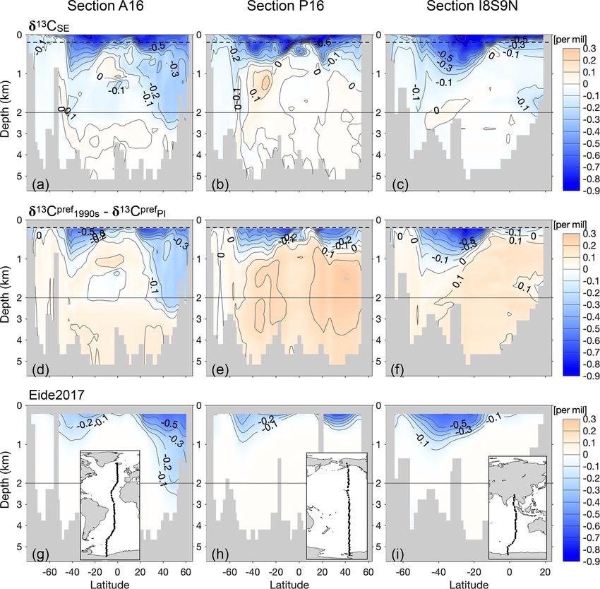
4392                                                                                      B. Liu et al.: 13 C module in MPI-ESM

in Eq. (6) the temperature dependency is weak, we use a con-
stant aq←g = −1.24, obtained at TC = 15 ◦ C in the model,
following Schmittner et al. (2013). In Eq. (7) we neglect the
first term 0.014TC fCO3 , because fCO3 is generally smaller
than 0.1 and because the constant factor is 1 order of magni-
tude smaller than that of the second term 0.105TC .
   Note that Eq. (5) (k = −0.85) and the simplified Eq. (7)
(DIC←g = −0.105 TC + 10.53) in this study, adopting those
of Schmittner et al. (2013), are slightly different from the
OMIP protocol (Orr et al., 2017; k = −0.88 and DIC←g =
0.014 TC fCO3 − 0.107 TC + 10.53). Results of a short pre-
industrial simulation with k and DIC←g from OMIP pro-
tocol yield a negligible difference (not shown). In our future
simulations k and DIC←g suggested by the OMIP protocol
will be used.

2.2.2    Fractionation during phytoplankton growth

The lighter stable carbon isotope 12 C is preferentially utilised   Figure 1. The per mil biological fractionation factor p against
                                                                                                                                Popp
over 13 C during photosynthesis (O’Leary, 1988). Following          aqueous CO2 concentration. The solid line illustrates p , in
Schmittner et al. (2013), we formulate this isotopic frac-          which the biological fractionation during phytoplankton growth is
tionation during net growth of the bulk phytoplankton and           only a function of CO2 (aq). The dashed–dotted lines show pLaws ,
cyanobacteria as                                                    which depends on µ/CO2 , the ratio of phytoplankton growth rate
                                                                    to CO2 (aq), for µ =0.2 (blue), 0.6 (red), 1.2 (yellow) and 2.0 (pur-
13
     G = RDIC αPhy←DIC G,                                    (8)    ple) d−1 .

with
                                                                    Both CO2 (aq) and µ (depending on local conditions of light,
                                    αaq←g
αPhy←DIC = αaq←DIC αPhy←aq =              αPhy←aq .          (9)    water temperature and nutrient availability) are determined
                                   αDIC←g                                                                               Popp
                                                                    in HAMOCC6. Figure 1 illustrates the values of p        and
                                                                    pLaws under typical ranges of CO2 (aq) and µ in the ocean.
Here G (µmol C L−1 d−1 ) denotes the growth of bulk phy-                                                                       Popp
                                                                    When µ ≤ 1, pLaws is generally more negative than p . For
toplankton or cyanobacteria. αPhy←DIC is the isotopic frac-
tionation factor for DIC fixation, which is determined by the       high µ values, e.g. µ = 2, pLaws is constantly less negative
                                                                            Popp
equilibrium fractionation factor αaq←DIC from DIC to aque-          than p . Under high µ and low CO2 (aq), pLaws becomes
ous CO2 (aq) and by the biological fractionation factor p =        positive, which is unrealistic. However, our simulated ratios
(αPhy←aq − 1) × 103 related to the fixation of CO2 (aq). Here       of phytoplankton growth rate to dissolved CO2 concentration
the subscript “Phy” denotes either the bulk phytoplankton or        do not produce unrealistic positive pLaws at any time step in
cyanobacteria.                                                      this study.
   We test the parameterisations for biological fractionation
from Popp et al. (1989) and from Laws et al. (1995), i.e.           2.3     Model setup and experimental design
 Popp
p     = −17 log(CO2 (aq)) + 3.4,                           (10)    2.3.1    Setup

                 µ
pLaws =                 − 0.371 /0.015.                    (11)    We conduct ocean-only simulations using the MPIOM-
           CO2 (aq)/ρsea
                                                                    1.6.3p1 (Jungclaus et al., 2013; Notz et al., 2013; Maurit-
                                                                    sen et al., 2019) with HAMOCC6. MPIOM is a free-surface
Here, CO2 (aq) (µmol L−1 ) is aqueous CO2 in surface wa-
                                                                    ocean general circulation model. It uses a curvilinear grid
ter, and variable µ (d−1 ) is the specific growth rate of
                                                                    with the grid poles located over Greenland and Antarctica.
bulk phytoplankton or of cyanobacteria. Note that Laws
                                                                    We use a low-resolution configuration with a nominal hori-
et al. (1995) measured aq←Phy . Because αPhy←aq is close
                                                                    zontal resolution of 1.5◦ . This configuration has a minimum
to unity, p ≈ −aq←Phy (Zeebe and Wolf-Gladrow, 2001).
                                                                    grid spacing of 15 km around Greenland and a maximum grid
In Eq. (11), we set the seawater density ρsea a constant value
                                                                    spacing of 185 km in the tropical Pacific. There are 40 un-
of 1.025 kg L−1 . Then Eq. (11) is simplified to
                                                                    evenly spaced vertical levels. The layer thickness increases
                  µ                                                 from 10 m in the upper ocean to 600 m in the deep ocean.
pLaws = 68.3            − 24.7.                            (12)    The upper 100 m of the water column is represented by nine
                CO2 (aq)

Biogeosciences, 18, 4389–4429, 2021                                                     https://doi.org/10.5194/bg-18-4389-2021
B. Liu et al.: 13 C module in MPI-ESM                                                                                         4393

levels. The time step is 1 h. In this setup, we additionally in-       In the transient simulations for the historical period 1850–
clude the oceanic uptake and transport of CFC-12. CFC-12            2010, Hist_Popp and Hist_Laws, we prescribe increasing
is chemically inert and can therefore be treated as a conser-       atmospheric CO2 mixing ratios (Meinshausen et al., 2017)
vative and passive tracer participating in all hydrodynamical       due to anthropogenic activities and decreasing atmospheric
processes within the ocean identical to e.g. salinity. The im-      δ 13 CO2 following OMIP and C4MIP protocols (Jones et al.,
plementation of the air–sea gas exchange of CFC-12 follows          2016) (Fig. 2a). For the period 1850–1900, when forcing data
the OMIP protocol (Orr et al., 2017).                               are absent, we continue applying the 1905–1929 ERA20C
                                                                    cyclic forcing. From 1901 to 2010, we use the transient
2.3.2   Experimental design                                         ERA20C forcing. The evolution of the atmospheric CFC-12
                                                                    concentration (Fig. 2b) follows Bullister (2017). Because the
For the pre-industrial spin-up simulations we cyclically ap-        atmospheric CFC-12 is slightly higher in the Northern Hemi-
ply the 1905–1929 sea-surface boundary conditions from              sphere, we prescribe a linear transition between 10◦ S and
ERA20C (Poli et al., 2016, covering 1901–2010). The at-             10◦ N. Input rates of DO13 C, DOC, 13 CO2−          2−
                                                                                                                3 , CO3 and SiO4
mospheric CO2 mixing ratio is set to 280 ppmv. A spin-up            are kept constant and are the same as those of pre-industrial
run is first conducted without 13 C tracers until the long-         simulations.
term averaged global net air–sea CO2 flux is smaller than
0.05 Pg C yr−1 (adequate to the C4MIP criterion for steady-
state conditions of < 0.1 Pg C yr−1 ; Jones et al., 2016). This
                                                                    3   Model results and observations in the late 20th
model state is the starting point for the two spin-up runs
                                                                        century
including 13 C tracers, PI_Popp and PI_Laws, which are
                                                            Popp
based on the biological fractionation parameterisation p           Our model generally simulates the physical and biogeochem-
(Eq. 10) and pLaws (Eq. 12), respectively.                         ical state for the present-day ocean well. The detailed model–
   The C tracers are initialised as follows. The mean δ 13 C
        13
                                                                    observation comparisons for the ocean physical variables
of the marine organic matter is about −20 ‰ (Degens et al.,         (e.g. seawater temperature and salinity, Atlantic Meridional
1968). Therefore, we set the initial concentrations of 13 C         Overturning Circulation stream function, CFC-12) and for
in the bulk phytoplankton, cyanobacteria, zooplankton, dis-         the ocean biogeochemical tracers (e.g. primary production,
solved organic carbon, particulate organic carbon in the wa-        nutrients, DIC) are summarised in Appendix Sects. B and C.
ter column and particulate organic carbon in the sediment to           In this section, we compare simulated 13 C between the
0.98 (according to Eq. 1) of their 12 C counterparts. The initial   two simulations Hist_Popp and Hist_Laws and evaluate the
13 C
    DIC in the water column is calculated using the relation        two experiments by comparison to observed δ 13 CPOC and
between δ 13 CDIC and PO4 (Lynch-Stieglitz et al., 1995),           δ 13 CDIC . The observations used here are the surface δ 13 CPOC
δ 13 CDIC = 2.7 − 1.1PO4 ,                                  (13)    measurements assembled by Goericke and Fry (1994) and
                                                                    the observed δ 13 CDIC , for both the surface and the interior
and Eq. (1). Here PO4 and DIC are from the quasi-                   ocean, compiled by Schmittner et al. (2013). For the model–
equilibrium state of the spin-up run without 13 C tracers. The      observation comparison, we first grid the observed δ 13 CPOC
initial concentrations of 13 CCaCO3 in the water column and in      and δ 13 CDIC horizontally onto a 1 × 1◦ grid and vertically
the sediment and the initial concentration of 13 CDIC in pore       (only for δ 13 CDIC ) onto the 40 depth layers of the model.
water are set identical to their 12 C counterparts.                 Multiple data points in the same grid cell in the same month
   The pre-industrial stable carbon isotope ratio δ 13 CO2 of       and year are averaged. Then we bilinearly interpolate the
atmospheric CO2 is fixed at −6.5 ‰. The inputs of dissolved         simulated monthly-mean δ 13 CPOC and δ 13 CDIC over a 1 × 1◦
organic 13 C (DO13 C) and 13 CO2−    3 are uniformly added at       grid. To quantitatively compare the performance between
the ocean surface. The input rate of DO13 C is calculated as        Hist_Popp and Hist_Laws and to other 13 C models, we cal-
the product of the input rate of DOC and the sea-surface            culate the spatial correlation coefficient r and the normalised
DO13 C/DOC ratio; the input rate of 13 CO2−    3 is the product     root mean squared error (NRMSE, normalised by the stan-
of the input rate of CO2−
                        3   and the  sea-surface 13 CO2− /CO2−
                                                      3      3      dard deviation that is calculated using all the available mea-
                                      13
ratio. This approach to determine C input rates results in a        surements of δ 13 CPOC or δ 13 CDIC during the observational
small drift in the water-column 13 C inventory, but it only has     periods) between model results and observation.
minor impact on the simulation results (see Appendix A).               A global ocean climatology of pre-industrial δ 13 CDIC has
   PI_Popp and PI_Laws are spun up for 2500 simula-                 recently been derived by first estimating the oceanic 13 C
tion years. Equilibrium states are reached with 98 % of             Suess effect (Eide et al., 2017a) and then removing it from
the ocean volume having a δ 13 CDIC drift of less than              the observed δ 13 CDIC (Eide et al., 2017b). This pre-industrial
0.001 ‰ yr−1 (employing the same criteria as for 14 C in            δ 13 CDIC estimate has been used to evaluate model perfor-
OMIP protocol, Orr et al., 2017). An equilibrium of the sed-        mance (Tjiputra et al., 2020). We do not include a δ 13 CDIC
iment is, however, not achieved for either 13 C or other bio-       evaluation for the pre-industrial ocean because the histori-
geochemical tracers.                                                cal simulations in this study facilitate the direct comparison

https://doi.org/10.5194/bg-18-4389-2021                                                    Biogeosciences, 18, 4389–4429, 2021
4394                                                                                        B. Liu et al.: 13 C module in MPI-ESM

Figure 2. (a) The evolution of atmospheric CO2 (blue, Meinshausen et al., 2017) and δ 13 CO2 (red, Jones et al., 2016) during 1850–2010.
(b) The evolution of atmospheric CFC-12 concentrations (Bullister, 2017). The solid blue line indicates the Northern Hemisphere, and the
dashed red line indicates Southern Hemisphere.

to observations in the late 20th century, which is different          of −29.9 ‰ due to more negative p (Fig. 3d). This is be-
from Tjiputra et al. (2020), who only include pre-industrial                                                              Popp
                                                                      cause pLaws (Fig. 1) is always more negative than p    when
simulations with 13 C tracers. Moreover, as has already been          the simulated mean growth rates (Fig. C1a and b) are lower
discussed by Eide et al. (2017a) and is discussed in Sect. 5          than 1 d−1 . As pLaws increases with growth rate (Eq. 12), we
of this study, the 13 C Suess effect is possibly underestimated       find less negative δ 13 CPOC (up to −24.1 ‰) in the central
by the Eide et al. (2017a) approach. This suggests Eide et al.        tropical Pacific, where highest growth rates are simulated
(2017b) likely overestimate the pre-industrial δ 13 CDIC .            (Fig. C1a and b). The lowest δ 13 CPOC of −33 ‰ occurs in
                                                                      the Arctic Ocean and around Antarctica due to the combina-
3.1    Isotopic signature of particular organic carbon in             tion of low growth rate, high CO2 (aq) and low seawater tem-
       the surface ocean                                              perature. The meridional range of the annual-mean δ 13 CPOC
                                                                      in Hist_Laws (∼ 9 ‰) is smaller than that of Hist_Popp
For comparison between Hist_Popp and Hist_Laws, the cli-              (∼ 11 ‰) because for low growth rates pLaws is generally
matological mean state of δ 13 CPOC is derived by averag-             less sensitive to CO2 (aq) changes compared to p
                                                                                                                          Popp
                                                                                                                             (Fig. 1).
ing over 1960-1991, the period when most δ 13 CPOC mea-               This also results in a smaller annual range of δ 13 CPOC in
surements were collected. In Hist_Popp, the climatological            high latitudes (Fig. 3f) than Hist_Popp (Fig. 3e). In the low
annual-mean surface δ 13 CPOC has a global mean value of              and mid-latitudes, Hist_Laws shows larger annual range of
−22.5 ‰, and it shows a distinct horizontal pattern (Fig. 3a).        δ 13 CPOC because in these regions CO2 (aq) concentrations
Less negative values up to −19.3 ‰ are found in the subtrop-          are relatively stable but growth rates shows noticeable sea-
ical regions, where alkalinity is typically high and CO2 (aq)         sonal variability.
is consequently low. This low CO2 (aq) results in a smaller              Hist_Popp captures major features of the observed
isotope fractionation during carbon fixation by phytoplank-           δ 13 CPOC (Fig. 4a, c and e). The meridional gradient, with
ton (Eq. 10, Fig. 1) with a biological fractionation factor           less negative values in the low latitudes and minimal val-
p > −13 ‰ (Fig. 3c). Poleward of the subtropical regions,            ues around 60◦ S, is well reproduced. In contrast, Hist_Laws
δ 13 CPOC gradually decreases. The reason for this is twofold.        shows generally lower δ 13 CPOC than the observations (a
First, p decreases from −13 ‰ to about −20 ‰ following               global mean bias of −8 ‰) and a smaller δ 13 CPOC differ-
the increase in CO2 (aq). Second, the thermal effect of equi-         ence between low and high latitudes (Fig. 4b, d and f). This
librium fractionation causes about 3 ‰ more fractionation in          is also seen in a recent study by Dentith et al. (2020), who
the polar regions than in the tropical and subtropical regions        tested p
                                                                                Popp
                                                                                     and pLaws with the FAst Met Office/UK Uni-
(according to Eqs. 7 and 9). The lowest δ 13 CPOC of about            versities Simulator (FAMOUS). The underestimation in the
−30 ‰ occurs close to Antarctica where highest surface DIC            global mean and in the meridional gradient of δ 13 CPOC in
concentrations are typically found because of the upwelling           Hist_Laws suggests that the parameters of the linear fit in
of deep waters and the reduced air–sea gas exchange by ice            Eq. (12) (slope and intercept) would need to be increased
cover (Takahashi et al., 2014). The annual range of δ 13 CPOC         to gain a better performance. Around 60◦ S of the Atlantic
(Fig. 3e), i.e. the difference between the minimum and the            Ocean (Fig. 4b), Hist_Laws simulates a smaller range of
maximum of its climatological monthly-mean annual cycle,              δ 13 CPOC than the observations. This is also a result of the
is low (< 0.5 ‰) in the subtropical regions, and it increases         small δ 13 CPOC annual range produced by pLaws (Fig. 3f). Be-
polewards up to ∼ 9 ‰ in the Southern Ocean, mirroring                tween 40◦ S and 40◦ N in the Atlantic Ocean, Hist_Laws sim-
meridional changes in the annual range of CO2 (aq).                   ulates δ 13 CPOC peaks in the region of high growth rates south
   Compared to Hist_Popp, Hist_Laws shows lower annual-
mean surface δ 13 CPOC (Fig. 3b), with a global-mean value

Biogeosciences, 18, 4389–4429, 2021                                                       https://doi.org/10.5194/bg-18-4389-2021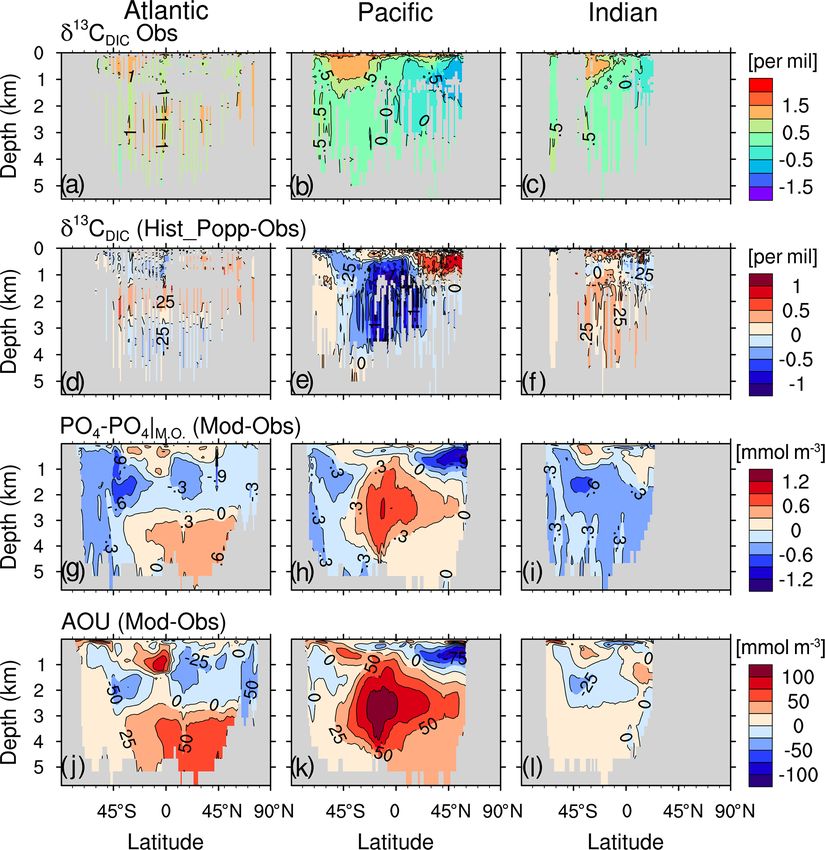
B. Liu et al.: 13 C module in MPI-ESM                                                                                              4395

Figure 3. The climatological (1960–1991) annual-mean surface values for Hist_Popp (a, c, e) and Hist_Laws (b, d, f) for δ 13 CPOC (a, b),
p (c, d), and for the annual range of δ 13 CPOC (e, f). All values are given in per mil (‰).

of the Equator, whereas the observed high δ 13 CPOC values             δ 13 CPOC peak to a local high phytoplankton production dur-
are located between the Equator and 20◦ N.                             ing the measurement period.
   In the Indian Ocean around 45◦ S, Hist_Popp does not cap-              Overall, Hist_Popp (r = 0.84 and NRMSE = 0.57) better
ture the prominent δ 13 CPOC peak in the field data (Fig. 4e),         reproduces the observed δ 13 CPOC than Hist_Laws (r = 0.71,
despite the fact that the simulated CO2 (aq), the controlling          NRMSE = 2.5). Here a higher NRMSE indicates the model
                                 Popp
factor in the parameterisation p     (Eq. 10), well reproduces        captures a smaller fraction of the variation in observations.
the meridional variation of the contemporaneous CO2 (aq)               The performance of Hist_Popp regarding δ 13 CPOC compares
measurements (Fig. 4g). Although the empirical correlation             well to that of the FAMOUS model (Dentith et al., 2020;
between p and CO2 (aq), such as Eq. (10), holds true to the           comparing their Fig. 8 and Fig. 4 in this study) and the Uni-
first order over large areas of the global ocean, other factors,       versity of Victoria (UVic) Earth System Model of intermedi-
such as growth rate, affect the local variability in p (Popp          ate complexity (with r = 0.74 and NRMSE = 0.92; Schmit-
et al., 1998; Hansman and Sessions, 2016; Tuerena et al.,              tner et al., 2013). Note that Schmittner et al. (2013) compared
2019). Hist_Laws captures the δ 13 CPOC peak around 45◦ S in           climatological annual-mean model output to the δ 13 CPOC
the observations (Fig. 4f), owing to the dependency of pLaws          measurements from Goericke and Fry (1994), whereas our
on phytoplankton growth rate and to the model successfully             study uses model results of the corresponding month and
reproducing the high productivity in this region (illustrated          year of the measurements. This difference leads to a better
by phytoplankton biomass, Fig. 4h). This is in alignment               comparison of Hist_Popp to the observed δ 13 CPOC in high
with the field study by Francois et al. (1993) and the model           latitudes, particularly in the South Atlantic Ocean around
study by Hofmann et al. (2000), who ascribed this observed             60◦ S, and therefore it is one reason for the slight better per-
                                                                       formance of Hist_Popp compared to Schmittner et al. (2013),

https://doi.org/10.5194/bg-18-4389-2021                                                        Biogeosciences, 18, 4389–4429, 2021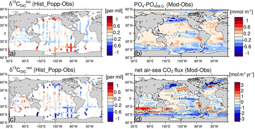
4396                                                                                           B. Liu et al.: 13 C module in MPI-ESM

Figure 4. Comparison of surface δ 13 CPOC (‰) observations (blue triangle) from Goericke and Fry (1994) to model data (red circle) in
Hist_Popp (a, c, e) and Hist_Laws (b, d, f) for the Atlantic, Pacific and Indian Ocean, respectively. Inserted maps show cruise tracks of the
measuring campaigns. (g) Comparison of simulated CO2 (aq) (red star) to observations (blue diamond) in the South Indian Ocean (Francois
et al., 1993; measurement locations indicated by black triangles in the inset map for the Indian Ocean). Panel (h) is as panel (g) but for
particulate organic matter, represented by total POC in Francois et al. (1993) and by phytoplankton biomass in the model. The measurement
precision is ±0.17 ‰ for δ 13 CPOC and 2 % for CO2 (aq) and particulate organic matter, according to Francois et al. (1993).

aside from the underlying differences between the two mod-               3.2     Isotopic signature of dissolved inorganic carbon
els.                                                                             δ 13 CDIC
   Hist_Popp also well reproduces the temporal changes of
the biological fractionation factor p when compared to                  3.2.1    Comparison between Hist_Popp and Hist_Laws
the observation-based estimates of Young et al. (2013). In                        and to observations
Hist_Popp, the change rate of p has a global-mean value of
−0.026 ‰ yr−1 for the period 1960–2009 (Fig. C7a), simi-                 Figures 5a–b and 6a–f compare the climatological annual
lar to an estimate of −0.022 ‰ yr−1 in Young et al. (2013).              mean of δ 13 CDIC (averaged over 1990–2005, when most
Modest p changes are found in eastern tropical Pacific and              δ 13 CDIC measurements were collected) between Hist_Popp
south of 60◦ S, in good agreement with Young et al. (2013).              and Hist_Laws. The two simulations exhibit very similar
Hist_Laws, on the other hand, shows a very small global-                 δ 13 CDIC patterns for both the surface and interior ocean. The
mean p change rate of −0.005 ‰ yr−1 (Fig. C7b) as pLaws                surface seawater DIC is enriched in 13 C due to the prefer-
is less sensitive to the increase in CO2 (aq) than p
                                                      Popp
                                                             .           ential uptake of the light isotope 12 C by phytoplankton dur-
                                                                         ing primary production. As particulate organic matter sinks
                                                                         and is remineralised at depth, the negative δ 13 CPOC signal is
                                                                         released. Consequently, in both Hist_Popp and Hist_Laws,
                                                                         δ 13 CDIC at the surface is generally higher than in the ocean

Biogeosciences, 18, 4389–4429, 2021                                                          https://doi.org/10.5194/bg-18-4389-2021
B. Liu et al.: 13 C module in MPI-ESM 4397
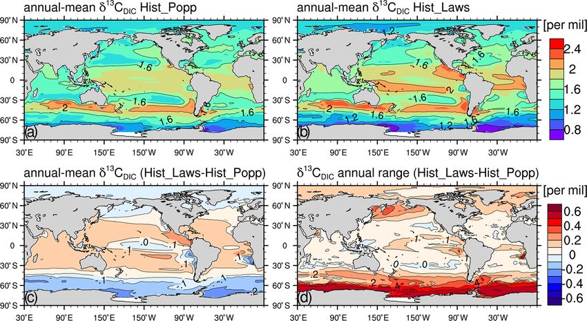
interior. At the surface of the equatorial central Pacific, the δ 13 CDIC into a biological component δ 13 Cbio
DIC and a residual
eastern boundary upwelling systems and the Southern Ocean component δ 13 Cresi
DIC , driven by air–sea exchange and ocean
south of 60◦ S, lower δ 13 CDIC (< 1.6 ‰) is seen due to the circulation:
upward transport of the 13 C-depleted water (Fig. 5a and b). 1photo
In the interior ocean, we find higher δ 13 CDIC (> 1 ‰) in δ 13 Cbio 13
DIC = δ CDIC |M.O. + RC:P (PO4 − PO4 |M.O. ). (14)
DICM.O.
well-ventilated water masses, in particular the North Atlantic
Deep Water (NADW) (Fig. 6a and d). The lowest δ 13 CDIC Here the subscript M.O. refers to mean ocean values, 1photo
values (< −0.5 ‰) occur at depth in tropical and subtropical is the carbon isotope fractionation during marine photosyn-
regions (Fig. 6a–f), where a large amount of organic matter thesis and RC:P is the C : P ratio of marine organic matter.
is remineralised. We use 1photo = −19 ‰ (Eide et al., 2017b) and RC:P =
The global-mean surface δ 13 CDIC of the two experiments 122 (Takahashi et al., 1985) for both model and observa-
only differs marginally (1.64 ‰ for Hist_Popp and 1.7 ‰ tional data. In reality 1photo shows spatial variability due to
for Hist_Laws), which is expected as they are run using the variations of CO2 (aq) (Fig. 3c) and temperature (Eq. 7)
the same prescribed atmospheric δ 13 CO2 (Schmittner et al., at the sea surface. However, using a constant 1photo only has
2013). Given very similar mean surface DI13 C, the larger limited quantitative impact on the model–observation com-
vertical DI13 C gradients in Hist_Laws, established by more parison of the two components. To calculate δ 13 Cbio DIC from
negative δ 13 CPOC (Fig. 3a and b), yield lower DI13 C con- observations, we employ δ 13 CDIC |M.O. = 0.5 ‰, DICM.O. =
centration at depth. This adjustment of DI13 C content in the 2255 mmol m−3 (Eide et al., 2017b) and PO4 from the World
ocean interior takes place during the pre-industrial spin-up Ocean Atlas (WOA13; Garcia et al., 2013a). Considering the
phase of the simulations via air–sea 13 CO2 exchange (Ap- strong seasonality in PO4 in the surface ocean, we select
pendix A). At the end of the 2500-year spin-up, the water- the phosphate concentration from the climatological monthly
column DI13 C inventory in PI_Laws is 1.1×10¹² kmol lower WOA data (available only for the upper 500 m of the wa-
than PI_Popp, yielding a global mean δ 13 CDIC difference ter column) and the climatological monthly-mean model
of 0.25 ‰ (Fig. 6g–i). Such interior-ocean δ 13 CDIC differ- data for the same month as the δ 13 CDIC observations. The
ence caused by using different parameterisation for biologi- observed mean ocean phosphate concentration PO4 |M.O. =
cal fractionation is also seen in Jahn et al. (2015) and Den- 1.7 mmol m−3 is obtained by first merging the time mean of
tith et al. (2020). The seasonal upward transport of the lower the PO4 monthly WOA data in the upper 500 m and the PO4
deep-ocean δ 13 CDIC in Hist_Laws leads to lower annual- annual-mean WOA data below 500 m and then mapping the
mean surface δ 13 CDIC and larger δ 13 CDIC annual range in combined data to the vertical grid of our model. For sim-
regions of upwelling (Fig. 5c and d). ulated δ 13 Cbio 13
DIC , the model data of δ CDIC |M.O. = 0.67 ‰,
When compared to the observed δ 13 CDIC , Hist_Popp (r = DICM.O. = 2197 mmol m−3 , PO4 |M.O. = 1.5 mmol m−3 and
0.81, NRMSE = 0.7) has a slightly better performance than PO4 are used. The model–observation δ 13 Cresi DIC difference
Hist_Laws (r = 0.80, NRMSE = 1.1). Hist_Laws generally is calculated by subtracting the model–observation δ 13 Cbio DIC
shows vertical gradients of δ 13 CDIC that are too strong and difference from the model–observation δ 13 CDIC difference.
therefore δ 13 CDIC values that are too low in the ocean inte- The model captures the major features of the observed
rior, as is seen in the depth profiles of horizontally averaged δ 13 Cbio
DIC at the surface; that is, higher values are seen in the
δ 13 CDIC (Fig. 7). This points to too strong a preference for subtropical regions and lower values in the high latitudes
the isotopically light carbon simulated by pLaws as is already (Fig. C8a and b). Nevertheless, noticeable quantitative dif-
discussed in Sect. 3.1. Given the slightly better performance ferences exist (Fig. 9a), which resemble the distribution of
of Hist_Popp than Hist_Laws regarding δ 13 CDIC , we focus (PO4 − PO4 |M.O. ) bias (Fig. 9b). Between 30◦ N and 30◦ S
in the following on the comparison between Hist_Popp and in the surface ocean, we find a mean negative bias of about
observed δ 13 CDIC . −0.1 ‰. This is caused by the underestimation of primary
production in the subtropical gyres (due to the underestima-
3.2.2 Source of surface δ 13 CDIC biases in Hist_Popp tion of phytoplankton growth rates; see Appendix C1) and
the consequently reduced enrichment of 13 C in surface DIC.
Figure 8 contains model–observation comparison for the sur- A strong positive δ 13 Cbio
DIC bias of 0.6 ‰ to 1 ‰ is seen in
face δ 13 CDIC . Overall, the magnitude and spatial distribu- the North Pacific, where in the model iron is not a limit-
tion of the observed δ 13 CDIC is well-captured by Hist_Popp. ing nutrient (Fig. C3), in contrast to observations (Moore
In the surface ocean, the mean δ 13 CDIC is slightly overesti- et al., 2013). In the equatorial central Pacific, a weak pos-
mated by Hist_Popp (1.7 ‰ compared to 1.5 ‰ in observa- itive δ 13 Cbio
DIC bias < 0.2 ‰ is caused by a primary produc-
tion). Positive biases are widely seen in the Indian and Pa- tion that is too high. Specifically, the simulated phytoplank-
cific Ocean, and the negative biases are mostly found in the ton growth rates in this region compare well to observations,
Atlantic Ocean (Fig. 8c). To better understand the source of whereas the simulated phytoplankton biomass is too high
differences between model and observations, we follow the (Appendix C1). The latter is mainly induced by an upwelling
method of Broecker and Maier-Reimer (1992) to decompose that is too strong. The observed mean upward vertical veloc-
https://doi.org/10.5194/bg-18-4389-2021 Biogeosciences, 18, 4389–4429, 2021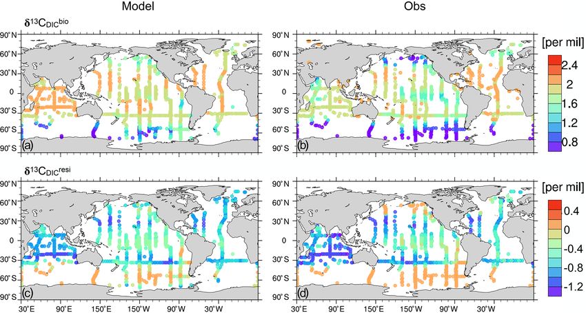
4398                                                                                            B. Liu et al.: 13 C module in MPI-ESM

Figure 5. Climatological (averaged over 1990–2005) annual-mean surface δ 13 CDIC for Hist_Popp (a) and Hist_Laws (b), respectively.
Panels (c) and (d) show the difference in the climatological annual-mean δ 13 CDIC between Hist_Laws and Hist_Popp, and the difference in
the climatological annual range of δ 13 CDIC between the two simulations, respectively.

Figure 6. Zonal-mean δ 13 CDIC of the Atlantic Ocean (a, d, g), the Pacific Ocean (b, e, h) and the Indian Ocean (c, f, i) for Hist_Popp (a–c),
Hist_Laws (d–f) and for the difference between Hist_Laws and Hist_Popp (g–i).

Biogeosciences, 18, 4389–4429, 2021                                                           https://doi.org/10.5194/bg-18-4389-2021
B. Liu et al.: 13 C module in MPI-ESM                                                                                                  4399

Figure 7. Depth profiles of horizontally averaged δ 13 CDIC of Hist_Popp (solid blue line), Hist_Laws (dashed red line) and the observational
data from Schmittner et al. (2013) (solid black line) for the global ocean (a), the Atlantic Ocean (b), the Pacific Ocean (c) and for the
Indian Ocean (d). The grey shading indicates observation uncertainty of ±0.15 ‰, which relates to the estimated accuracy due to unresolved
intercalibration issues between laboratories (0.1 ‰–0.2 ‰; Schmittner et al., 2013).

Figure 8. Observed surface δ 13 CDIC (Schmittner et al., 2013) (a) and simulated δ 13 CDIC in Hist_Popp sampled at the location, month and
year of the observation (b). (c) The difference in δ 13 CDIC between Hist_Popp and observations.

ity at 0, 140◦ W and 60 m depth during May 1990–June 1991                itive apparent oxygen utilisation (AOU) biases above 500 m
is 2.3 × 10⁻⁵ m s−1 (Weisberg and Qiao, 2000), whereas the               south of 45◦ S (Fig. 10j–l).
model simulates 3.2 × 10⁻⁵ m s−1 for the same location and                  Another reason for the high surface iron concentration in
period.                                                                  the Southern Ocean is that MPIOM simulates an upwelling
   In the Southern Ocean, a strong positive δ 13 Cbio
                                                  DIC bias of            that is too strong. In particular, below 1000 m, the simu-
0.6 to 1 ‰ (Fig. 9a) results from a primary production that is           lated upward velocity shows noticeably larger magnitude
too high under surface iron concentrations that are too high             (> 5 × 10⁻⁶ m s−1 , Fig. B4) than that of a dynamically con-
(0.2–0.4 nmol L−1 compared to generally < 0.25 nmol L−1                  sistent and data-constrained ocean state estimate (see Fig. 1
from data of the GEOTRACES programme (http://www.                        in Liang et al., 2017). The upwelling that is too strong in
geotraces.org, last access: 15 April 2021, not shown). Pri-              the model is consistent with the volume transport that is
mary production is limited by iron only south of 50◦ S in the            too large across the Drake Passage of 192 Sv compared to
model compared to south of 40◦ S from observation (Moore                 134–173 Sv from observations (Nowlin Jr. and Klinck, 1986;
et al., 2013). One cause for the high surface iron concentra-            Cunningham et al., 2003; Meredith et al., 2011; Donohue
tion is that in HAMOCC6 organic matter is remineralised at               et al., 2016). Our model also features larger downward veloc-
depths that are too shallow. This can been seen from the pos-            ities than the estimate from Liang et al. (2017), which corre-
                                                                         spond to mixed layer depths that are too deep in the Southern

https://doi.org/10.5194/bg-18-4389-2021                                                           Biogeosciences, 18, 4389–4429, 2021
4400 B. Liu et al.: 13 C module in MPI-ESM
Figure 9. Model–observation difference in the biological component δ 13 Cbio DIC (a), (PO4 − PO4 |M.O. ) (b), and the residual component
δ 13 Cresi
DIC (c) at the ocean surface. (d) The net air–sea CO2 flux (positive into the air, averaged over 1990–2005) difference between the model
data and observation-based data product from Landschützer et al. (2015).
Ocean (up to 3000 m, Fig. B5) than observations (< 700 m; caused by a remineralisation that is too low, as is shown by
de Boyer Montégut et al., 2004; Holte et al., 2017). the negative AOU biases (Fig. 10j–l).
We find strong δ 13 Cresi
DIC negative biases of −0.5 ‰ to North of 30◦ S in the Atlantic Ocean, the negative δ 13 CDIC
−1 ‰ (Fig. 9c) in the North Pacific and the Southern Ocean, biases below 3000 m, together with the positive δ 13 CDIC bi-
which partially compensate for the positive biases of δ 13 Cbio
DIC ases between 1000 and 3000 m, suggest δ 13 CDIC vertical gra-
(Fig. 9a) in these regions. One major cause for the nega- dients that are too strong in the model (Fig. 10d). This results
tive δ 13 Cresi
DIC bias in these two regions is our model over- from a lower boundary of the NADW cell that is too shallow,
estimating the uptake of anthropogenic carbon, as is illus- constantly located above 2800 m (Fig. B3), compared to an
trated by the net air–sea CO2 difference between the model estimated NADW lower boundary of about 4300 m deep at
and the observation (Fig. 9d). Consequently, the decreased 26◦ N (Msadek et al., 2013; Smeed et al., 2017). A possi-
atmospheric 13 C/12 C ratio over the industrial period further ble reason for the shallow NADW in the model is that the
lowers δ 13 CDIC in the two ocean regions in the model. In the Lower North Atlantic Deep Water (LNADW), forming from
Southern Ocean, the upward transport of 13 C-depleted wa- the Denmark Strait Overflow Water and the Iceland–Scotland
ter is too large, which also contributes to a negative δ 13 Cresi
DIC Overflow Water, is not dense enough to flow further south-
bias. ward. This can be seen from the CFC-12 distribution along
the zonal Sect. A5 at 24◦ N (Fig. B7). The observed deeper
CFC-12 maximum (3000–4500 m west of 60◦ W) indicates
3.2.3 Source of δ 13 CDIC biases in the interior ocean of the presence of LNADW (Dutay et al., 2002), which is not
Hist_Popp represented in our model.
We find the strongest negative δ 13 CDIC bias in the deep
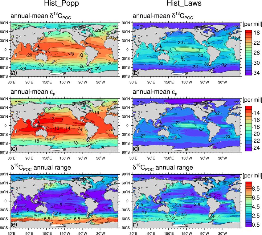
Figure 10 contains the model–observation comparison for eastern equatorial Pacific (Fig. 10e). The cause is the “nu-
zonal-mean δ 13 CDIC in the Atlantic, Pacific and Indian trient trapping” problem in the model, characterised by nu-
Ocean. In the interior ocean, δ 13 CDIC is controlled by rem- trient concentrations that are too high in the deep eastern
ineralisation of 13 C-depleted organic matter and by ocean equatorial Pacific (Fig. 10h), which is a persistent problem
circulation (Broecker and Peng, 1993; Lynch-Stieglitz et al., in many ESMs (Aumont et al., 1999; Dietze and Loeptien,
1995; Schmittner et al., 2013). Low δ 13 CDIC is often found 2013). Based on sensitivity experiments with the Geophysi-
in waters of high nutrient concentration and vice versa. Thus, cal Fluid Dynamics Laboratory model and the UVic model,
we find positive (negative) δ 13 CDIC biases coincide with neg- Dietze and Loeptien (2013) concluded the primary cause of
ative (positive) phosphate biases (Fig. 10d–i). In the At- the nutrient trapping problem is likely model biases in phys-
lantic Ocean between 1000 and 3000 m, the North Pacific ical ocean state – in particular, the poor representation of the
above 1500 m and the Indian Ocean below 1000 m, posi- Equatorial Intermediate Current system and equatorial deep
tive δ 13 CDIC biases and negative phosphate biases are mainly jets. The latter two current systems are indeed poorly repre-
Biogeosciences, 18, 4389–4429, 2021 https://doi.org/10.5194/bg-18-4389-2021B. Liu et al.: 13 C module in MPI-ESM 4401 Figure 10. Zonal-mean distribution in the Atlantic Ocean (left column), the Pacific Ocean (middle column) and the Indian Ocean (right column) for the δ 13 CDIC observations from Schmittner et al. (2013) (a–c), for the difference between Hist_Popp (sampled at the same location, year and month of the observations) and δ 13 CDIC measurement (d–f), for the (PO4 − PO4 |M.O. ) difference between model and WOA data (WOA13; Garcia et al., 2013a) (g–i), and for the apparent oxygen utilisation (AOU) difference between model and WOA data (WOA13; Garcia et al., 2013b) (j–l). Here the climatological annual mean values of PO4 and AOU are used for both model and WOA data because seasonal variation is negligible in the interior ocean and WOA only provides monthly data above 500 m. sented in our model as well. Specifically, the zonal current Jahn et al., 2015; comparing their Figs. 5 and 6 to our at 1000 m depth (typical depth for the Equatorial Interme- Figs. 7 and 6, respectively), and the UVic Earth System diate Current system) shows too little spatial variability and Model (Schmittner et al., 2013). The latter two studies used too low speeds of ∼ 0.2 cm s−1 (Fig. B6), compared to the the same δ 13 CDIC data set for model evaluation. Schmittner observed alternating jets with a meridional scale of 1.5◦ and et al. (2013) reported a better performance (r = 0.88 and speeds of ∼ 5 cm s−1 (see Fig. 2 from Cravatte et al., 2012). NRMSE = 0.5) than ours (r = 0.81 and NRMSE = 0.7 in The performances of both Hist_Popp and Hist_Laws re- Hist_Popp). One main reason is that the nutrient trapping garding δ 13 CDIC are comparable with the Norwegian Earth problem in HAMOCC6 does not occur in the simulations of System Model version 2 (NorESM2, Tjiputra et al., 2020; Schmittner et al. (2013). comparing their Fig. 21), the Commonwealth Scientific and Industrial Research Organisation Mark 3L climate system model with the Carbon of the Ocean, Atmosphere and Land 4 Evaluation of the simulated oceanic 13 C Suess effect (CSIRO Mk3L-COAL), Pelagic Interactions Scheme for Carbon and Ecosystem Studies (PISCES) and LOch-Vecode- The oceanic δ 13 C measurements taken during the late 20th Ecbilt-CLio-agIsm Model (LOVECLIM) (see Table 2 and century already include a signal that originates from burn- Figs. 3, S2 and S3 of Buchanan et al., 2019, and refer- ing of isotopically light fossil fuel over the industrial period. ences therein), the Community Earth System Model (CESM, The associated decrease in atmospheric δ 13 C (Fig. 2) affects https://doi.org/10.5194/bg-18-4389-2021 Biogeosciences, 18, 4389–4429, 2021
4402                                                                                             B. Liu et al.: 13 C module in MPI-ESM

                                                                                    C
oceanic δ 13 C via air–sea gas exchange, leading to a general            The       −O2 org   ratio is 122 : 172 in HAMOCC6, and we use
decrease in δ 13 CDIC . The distribution of this δ 13 CDIC change,
                                                                         the simulated δ 13 CPOC for δ 13 Corg . Clearly, the change in the
i.e. the oceanic 13 C Suess effect, could serve as benchmark                                           pref         pref         pref
for ocean models to evaluate the uptake and re-distribution              preformed component δ 13 CSE = δ 13 C1990s − δ 13 CPI dom-
                                                                                   13
                                                                         inates δ CSE (comparing Fig. 12a–c to Fig. 12d–f). A ma-
of the anthropogenic CO2 emissions in the ocean.
                                                                                                        pref
   The model is able to reproduce the size of the global                 jor difference between δ 13 CSE and δ 13 CSE is that positive
                                                                               pref
oceanic anthropogenic CO2 sink, though some local biases                 δ 13 CSE is widely seen below 1000 m, particularly in the Pa-
in the net air–sea CO2 flux exist (Fig. 9d). The simulated                                                                pref
                                                                         cific Ocean (Fig. 12e). These positive δ 13 CSE values relate
sink by year 1994 is 99 Pg C, which compares well to the                 to changes in the regenerated component δ 13 Creg (see Ap-
observation-based estimate of 118 ± 19 Pg C from Sabine                  pendix D).
et al. (2004) and to other model estimates (e.g. 94 Pg C
in Tagliabue and Bopp, 2008). For a direct comparison to
published studies, we calculate the oceanic δ 13 C Suess ef-             5   Potential sources of uncertainties in an
fect, δ 13 CSE , as the difference between the 1990s-averaged                observation-based global oceanic 13 C Suess effect
δ 13 CDIC from Hist_Popp and the pre-industrial climatolog-                  estimate
ical (50-year mean) δ 13 CDIC from PI_Popp. δ 13 CSE calcu-
lated using the results of Hist_Laws and PI_Laws only shows              Eide et al. (2017a) (hereafter E17) derived the first
a marginal difference (global mean < 0.04 ‰) and is there-               observation-based estimate of the global ocean 13 C Suess
fore not presented.                                                      effect since pre-industrial times. E17’s approach uses the
   The surface mean δ 13 CSE in this study is −0.66 ‰, similar           concept of the similarity between the oceanic uptake of the
to the model study of Schmittner et al. (2013) (−0.67 ‰) and             anthropogenically produced CFC-12 and isotopically light
to the estimate by Sonnerup et al. (2007) (−0.76 ± 0.12 ‰),              CO2 (see details in Appendix E1). Due to method- and data-
who used an observation-based approach. The strongest                    specific limitations E17 stated that they potentially underesti-
oceanic 13 C Suess effect is found in the subtropical gyres              mate the oceanic 13 C Suess effect. However, based on obser-
in the model (Fig. 11a), where water masses have long res-               vations alone it is not possible to gain insight into the spatial
idence times at the ocean surface and therefore receive a                distribution of this uncertainty or into its origin.
strong anthropogenic imprint (Quay et al., 2003). In the                    Our model simulations, particularly PI_Popp and
subtropical gyres, the simulated surface δ 13 CSE generally              Hist_Popp, provide an opportunity to learn more about the
varies between −0.8 ‰ and −1.1 ‰, which compares well                    source of this uncertainty because the oceanic δ 13 C in the
to the surface ocean δ 13 C decrease of −0.9±0.1 ‰ recorded              late 20th century (Sect. 3), the oceanic anthropogenic CO2
by coral and sclerosponges (Wörheide, 1998; Böhm et al.,                 sink (Sect. 4) and the invasion of CFC-12 into the ocean
1996, 2000; Swart et al., 2002, 2010) and to the estimates               (Fig. B8) are well represented. Moreover, our simulated
of −1.0 ± 0.09 ‰ extracted from GLODAPv2 (Olsen et al.,                  δ 13 CSE qualitatively resembles the oceanic 13 C Suess effect
2016; Eide et al., 2017a).                                               estimate of E17 (see comparison between Fig. 11b and E17’s
   Along the vertical sections A16, P19 and I8S9N, δ 13 CSE              Fig. 7, as well as comparison between Fig. 12a–c and g–i).
is mainly confined to the upper 1000 m depth in the sub-                    Based on the similarity between the oceanic uptake of the
tropical gyres of the South Atlantic, the Pacific Ocean and              atmospheric CFC-12 and δ 13 CO2 signal, E17 link the 13 C
the Indian Ocean (Fig. 12a–c). In the North Atlantic, δ 13 CSE           Suess effect since 1940 (when CFC-12 becomes detectable
penetrates deeper than the other ocean regions, due to the               in the ocean) to CFC-12 partial pressure (pCFC-12) with
intensive ventilation related to the formation of NADW. The              a proportionality factor. Under the assumption of a tempo-
simulated δ 13 CSE distributions show similar features to those          rally constant regenerated fraction δ 13 Creg , this proportion-
of CFC-12 (Fig. B8). This is because both the decrease in                ality factor is considered equivalent to the slope of a linear
δ 13 CDIC and increase in CFC-12 in the ocean are predom-                regression relationship between the preformed component
inantly caused by the uptake of atmospheric anthropogenic                δ 13 Cpref and pCFC-12 at any time after 1940. Thus, this slope
signals and the subsequent transport by ocean circulation.               a can be obtained by performing linear regression for field
Since changes in δ 13 CDIC are also induced by changes in                measurements of δ 13 Cpref and pCFC-12. Multiplying a and
marine biological activity, we separate δ 13 CDIC into a com-            pCFC-12 data yields the 13 C Suess effect since 1940, which
ponent depicting changes due to the transport of the surface             is then scaled to the full industrial period by a constant fac-
13 C signal, i.e. the “preformed” δ 13 C
                                          DIC , and to a regener-
                                                                         tor fatm (Eq. E7) related to changes in the atmospheric δ 13 C
ated component δ 13 Creg , following Sonnerup et al. (1999):             signature:
                                                                         δ 13 CSE(t−PI) = fatm · a · pCFC-12t .                       (16)

                                              C
               δ 13 CDIC · DIC − AOU ·                  13
                                             −O2 org · δ Corg            Here a is the regression slope for the linear relationship be-
 13 pref                                                                             pref
δ C        =                                                  . (15)   tween δ 13 Ct and pCFC-12t (Eq. E5). The value of a is de-
                                              C
                        DIC − AOU ·          −O2 org                     termined for each ventilation region defined in E17 (i.e. the

Biogeosciences, 18, 4389–4429, 2021                                                            https://doi.org/10.5194/bg-18-4389-2021
You can also read