Wintertime direct radiative effects due to black carbon (BC) over the Indo-Gangetic Plain as modelled with new BC emission inventories in CHIMERE
←
→
Page content transcription
If your browser does not render page correctly, please read the page content below
Atmos. Chem. Phys., 21, 7671–7694, 2021
https://doi.org/10.5194/acp-21-7671-2021
© Author(s) 2021. This work is distributed under
the Creative Commons Attribution 4.0 License.

Wintertime direct radiative effects due to black carbon (BC)
over the Indo-Gangetic Plain as modelled with new BC
emission inventories in CHIMERE
Sanhita Ghosh1 , Shubha Verma2 , Jayanarayanan Kuttippurath3 , and Laurent Menut4
1 Advanced   Technology Development Centre, Indian Institute of Technology Kharagpur, Kharagpur-721302, India
2 Department  of Civil Engineering, Indian Institute of Technology Kharagpur, Kharagpur-721302, India
3 Centre for Oceans, Rivers, Atmosphere and Land Sciences (CORAL), Indian Institute of Technology Kharagpur,

Kharagpur-721302, India
4 Laboratoire de Météorologie Dynamique, IPSL, CNRS/Ecole Polytechnique/Sorbonne Université/Ecole Normale

Supérieure, 91128 Palaiseau CEDEX, France

Correspondence: Shubha Verma (shubha@iitkgp.ac.in)

Received: 27 June 2020 – Discussion started: 25 September 2020
Revised: 30 March 2021 – Accepted: 31 March 2021 – Published: 20 May 2021

Abstract. To reduce the uncertainty in climatic impacts         strained estimated BC concentration (NMB: < 17 %) and
induced by black carbon (BC) from global and regional           aerosol optical depth due to BC (BC-AOD) (NMB: 11 %)
aerosol–climate model simulations, it is a foremost re-         indicated that simulations with Constrainedemiss BC emis-
quirement to improve the prediction of modelled BC dis-         sions in CHIMERE could simulate the distribution of BC
tribution, specifically over the regions where the atmo-        pollution over the IGP more efficiently than with bottom-up
sphere is loaded with a large amount of BC, e.g. the Indo-      emissions. The high BC pollution covering the IGP region
Gangetic Plain (IGP) in the Indian subcontinent. Here we        comprised a wintertime all-day (daytime) mean BC concen-
examine the wintertime direct radiative perturbation due        tration and BC-AOD respectively in the range 14–25 µg m−3
to BC with an efficiently modelled BC distribution over         (6–8 µg m−3 ) and 0.04–0.08 from the Constrained simula-
the IGP in a high-resolution (0.1◦ × 0.1◦ ) chemical trans-     tion. The simulated BC concentration and BC-AOD were in-
port model, CHIMERE, implementing new BC emission in-           ferred to be primarily sensitive to the change in BC emis-
ventories. The model efficiency in simulating the observed      sion strength over most of the IGP (including the megacity
BC distribution was assessed by executing five simula-          of Kolkata), but also to the transport of BC aerosols over
tions: Constrained and bottomup (bottomup includes Smog,        megacity Delhi. Five main hotspot locations were identified
Cmip, Edgar, and Pku). These simulations respectively im-       in and around Delhi (northern IGP), Prayagraj–Allahabad–
plement the recently estimated India-based observationally      Varanasi (central IGP), Patna–Palamu (mideastern IGP), and
constrained BC emissions (Constrainedemiss ) and the latest     Kolkata (eastern IGP). The wintertime direct radiative per-
bottom-up BC emissions (India-based: Smog-India; global:        turbation due to BC aerosols from the Constrained simula-
Coupled Model Intercomparison Project phase 6 – CMIP6,          tion estimated the atmospheric radiative warming (+30 to
Emission Database for Global Atmospheric Research-V4 –          +50 W m−2 ) to be about 50 %–70 % larger than the surface
EDGAR-V4, and Peking University BC Inventory – PKU).            cooling. A widespread enhancement in atmospheric radiative
The mean BC emission flux from the five BC emission in-         warming due to BC by 2–3 times and a reduction in surface
ventory databases was found to be considerably high (450–       cooling by 10 %–20 %, with net warming at the top of the
1000 kg km−2 yr−1 ) over most of the IGP, with this being the   atmosphere (TOA) of 10–15 W m−2 , were noticed compared
highest (> 2500 kg km−2 yr−1 ) over megacities (Kolkata and     to the atmosphere without BC, for which a net cooling at the
Delhi). A low estimated value of the normalised mean bias       TOA was exhibited. These perturbations were the strongest
(NMB) and root mean square error (RMSE) from the Con-           around megacities (Kolkata and Delhi), extended to the east-

Published by Copernicus Publications on behalf of the European Geosciences Union.
7672                              S. Ghosh et al.: Wintertime direct radiative effects of BC over the Indo-Gangetic Plain

ern coast, and were inferred to be 30 %–50% lower from the       simulated BC concentration exhibited a consistent correla-
bottomup than the Constrained simulation.                        tion with, but was significantly lower (by a factor of about
                                                                 2 to 11) than, the measured concentration (Kumar et al.,
                                                                 2018; Verma et al., 2017; Kumar et al., 2015; Pan et al.,
                                                                 2015; Sanap et al., 2014; Moorthy et al., 2013; Nair et al.,
1   Introduction                                                 2012). The factor of model underestimation was further no-
                                                                 ticed to be large, specifically during wintertime over the
Black carbon (BC) is released into the atmosphere from the       Indo-Gangetic Plain (IGP) when the atmosphere is observed
incomplete combustion of carbon-based fuels (Bond et al.,        to be laden with a large BC burden.
2013; Verma et al., 2013; Sadavarte and Venkataraman,               To assess BC aerosol absorption accurately and reduce the
2014). It is one of the constituents of concern among the        uncertainty in the BC DRF as estimated from global and re-
atmospheric aerosol pollutants because of its profound im-       gional aerosol–climate models, it is therefore a foremost re-
pact on climate through an imbalance of the Earth’s radia-       quirement to improve the prediction of atmospheric BC es-
tion budget, in addition to degradation of air quality and ad-   timates in models, specifically over regions where the atmo-
verse effects on human health (Qian et al., 2011; Wang et al.,   sphere is loaded with a large amount of BC, e.g. the Indo-
2014a; Fan et al., 2015; Zhang et al., 2015; Janssen et al.,     Gangetic Plain (IGP) in the Indian subcontinent (Nair et al.,
2011, 2012). Among aerosol constituents, BC aerosols are         2007; Verma et al., 2013; Ram and Sarin, 2015; Thamban
considered the strongest absorber of visible solar radiation     et al., 2017; Rana et al., 2019). Possible reasons suggested
and thereby a prominent contributor to tropospheric warming      for the discrepancy between models and observations have
as for the greenhouse gases – carbon dioxide and methane         included lack of BC emissions used as input, inadequate me-
(Ramanathan and Carmichael, 2008; Gustafsson and Ra-             teorology and representation of aerosol treatment, and coarse
manathan, 2016; Masson-Delmotte et al., 2018). However,          resolution in the model (e.g. Santra et al., 2019; Kumar et al.,
the magnitude of tropospheric radiative warming due to BC        2018; Wang et al., 2016; Pan et al., 2015; Verma et al., 2011;
aerosols is highly uncertain and is classified with medium-      Reddy et al., 2004).
to low-level understanding in the Intergovernmental Panel           However, it is also noted from the evaluation of BC con-
on Climate Change Fifth Assessment Report (IPCC AR5)             centration estimated from the free-running aerosol simula-
(Myhre et al., 2013a, b; Wang et al., 2016; Boucher et al.,      tions using the Laboratoire de Météorologie Dynamique at-
2016; Permadi et al., 2018a; Paulot et al., 2018; Dong et al.,   mospheric general circulation model (LMDZT-GCM) that
2019). The direct radiative forcing (DRF) of BC averaged         simulated BC, which is underestimated by a significant fac-
over the globe is estimated in the range 0.2–1 W m−2 (Myhre      tor at stations close to emission sources (such as that over
et al., 2013b; Bond et al., 2013; Gustafsson and Ramanathan,     mainland India), exhibits a relatively lower discrepancy with
2016). These estimates from global climate models used in        observed BC concentrations over the Indian oceanic regions
the latest assessment by the IPCC is noted to be about 2 times   (Reddy et al., 2004; Verma et al., 2007, 2011). The simulated
lower than observation-based estimates from satellite and        BC distribution from LMDZT-GCM was also found to con-
ground-based Aerosol Robotic Network (AERONET) obser-            sistently match the available observations at high-altitude Hi-
vations (0.7–0.9 W m−2 ) (Chung et al., 2012; Myhre et al.,      malayan Hindukush stations (e.g. Hanle, Satopanth), which
2013b; Gustafsson and Ramanathan, 2016; Stocker et al.,          are relatively remotely located and mostly influenced by the
2014). The DRF of BC is also inferred to be uncertain (e.g.      transport of aerosols (Santra et al., 2019). The above evalua-
−0.06 to +0.22 W m−2 ) when estimated for BC-rich sources        tions therefore suggest that the large underestimation of BC
comprising BC emitted with different compositions of short-      concentration over the Indian mainland would primarily be
lived co-emissions of species, e.g. sulfate and organic carbon   due to BC emission datasets instead of the model configura-
(Bond et al., 2013).                                             tions.
   Though consensus is still to be achieved on BC DRF,              The simulated atmospheric BC burden with atmospheric
nevertheless, the global atmospheric absorption attributable     chemical transport models is related to the BC emission
to BC was found to be too low in models and had to be            strength as input and simulated atmospheric residence time
enhanced by a factor of 3 to converge with observation-          of BC (Textor et al., 2006). While the atmospheric resi-
based estimates (Bond et al., 2013). The systematic under-       dence time of BC aerosols is independent of the emission
estimation of BC aerosol absorption by global climate model      strength, it is an indication of model-specific treatments of
predictions relative to atmospheric observations as noticed      transport and aerosol processes affecting the simulated BC
specifically over southern Asia and eastern Asia (Chung          burden. The uncertainty in the mean model residence time
et al., 2012; Gustafsson and Ramanathan, 2016) is also in        for BC based on evaluation in 16 global aerosol models
compliance with studies evaluating atmospheric BC concen-        has been estimated as 33 % (Textor et al., 2006), which is
trations between models and observations. For example, re-       noted to be much lower than the discrepancy found between
cent evaluations of BC concentration from global and re-         the simulated BC and observations. Due to the inclusion of
gional aerosol models over southern Asia showed that the         various complex physical–chemical atmospheric and aerosol

Atmos. Chem. Phys., 21, 7671–7694, 2021                                            https://doi.org/10.5194/acp-21-7671-2021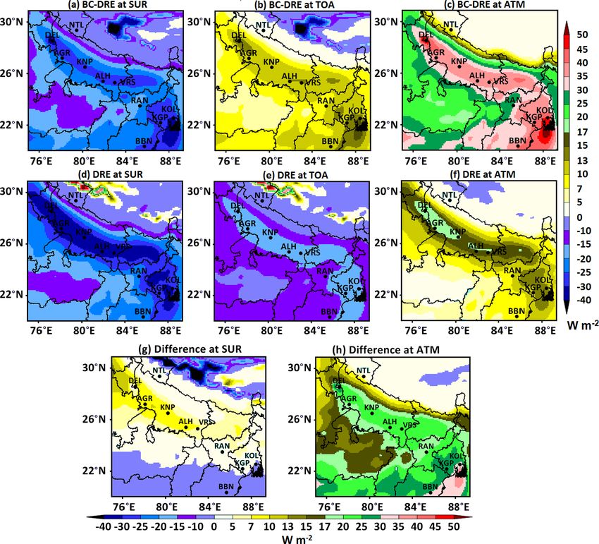
S. Ghosh et al.: Wintertime direct radiative effects of BC over the Indo-Gangetic Plain                                      7673

processes in these models, in conjunction with the inherent       depth due to BC (BC-AOD) and its fractional contribution to
uncertainty in inputs to the model (e.g. aerosol emissions        total AOD are also examined, in conjunction with present-
and their properties), a systematic approach is required to im-   ing an analysis of the wintertime radiative perturbation due
prove the prediction of BC aerosols in the models. The un-        to BC aerosols. Note that applications presented in this pa-
certainty in the bottom-up BC emission inventory has been         per focus on aerosol–radiation interactions only and show the
inferred to be greater than 200 % over India and Asia (Bond       wintertime direct radiative perturbations or the direct radia-
et al., 2004; Streets et al., 2003; Venkataraman et al., 2005;    tive effects (DREs) due to BC. The study of indirect aerosol
Lu et al., 2011) compared to about 40 % in recently es-           effects referring to cloud–aerosol interactions and evaluating
timated Constrainedemiss BC emissions over India (Verma           changes in the number of cloud condensation nuclei, includ-
et al., 2017). Therefore, in the above context, it is required    ing perturbations of the cloud albedo and rainfall (Boucher
to assess the efficacy of simulating the BC burden in a state-    et al., 2013; Lohmann and Feichter, 2005), is currently on-
of-the-art chemical transport model under different emis-         going and shall be presented in a forthcoming study.
sion scenarios (e.g. bottom-up and Constrainedemiss ) evaluat-       The specific objectives of this study are therefore the fol-
ing the divergence in BC emission flux from state-of-the-art      lowing:
bottom-up BC emission inventories and Constrainedemiss BC
emissions.                                                             i. characterise the model efficiency from five simulations
   In this study, we examine the wintertime direct radia-                 through a detailed validation and statistical analysis of
tive effects of BC over the IGP by evaluating the efficacy                simulated BC concentration with respect to ground-
of simulated atmospheric BC burden in a high-resolution                   based measurements at stations over the IGP and iden-
(0.1◦ × 0.1◦ ) chemical transport model, CHIMERE, during                  tify the regional hotspots;
winter when a large BC burden is observed. This is done by
executing multiple BC transport simulations with CHIMERE              ii. utilise the multi-simulations to quantify the degree of
and implementing new BC emission inventories, which in-                   variance in estimated BC concentration attributed to
clude the recently estimated India-based Constrainedemiss                 emissions corresponding to areas types (e.g. megacity,
BC emissions and the latest bottom-up BC emissions (India-                urban, semi-urban, low-polluted) and temporal distribu-
based: Speciated Multi-pOllutant Generator – Smog-India;                  tion (e.g. daytime and evening hours);
global: Coupled Model Intercomparison Project Phase 6 –
                                                                   iii. evaluate the spatial features of BC-AOD from five sim-
CMIP6, Emission Database for Global Atmospheric Re-
                                                                        ulations and analyse the association between simu-
search V4 – EDGAR V4, and the Peking University – PKU–
                                                                        lated BC concentration and BC-AOD with BC emission
BC inventory). A short description of the five BC emission
                                                                        strength; and
datasets is provided in Sect. 2.1. The bottom-up BC emis-
sions applied in the present study are being widely used              iv. examine the spatial distribution of wintertime radiative
in regional and global climate models in the assessment of                perturbation due to BC aerosols over the IGP compared
the spatial and temporal distribution of aerosol burden and               to the atmosphere considered without BC aerosols.
aerosol–climate interactions (Eyring et al., 2016; Zhou et al.,
2020; David et al., 2018; Lamarque et al., 2010; Meng et al.,
2018; Wang et al., 2016), including e.g. CMIP6, to support        2     Method of study
the IPCC climate assessment report (Myhre et al., 2013a).
Henceforth, it is necessary to evaluate the performance of the    2.1     Experimental set-up for simulating BC surface
new BC emissions (bottom-up and Constrainedemiss ) with a                 concentrations
state-of-the-art chemical transport model for their adequacy
to represent the BC distribution and thereby the climatic im-     High-resolution BC transport simulations are carried out
pacts over the IGP in the Indian subcontinent. The model ef-      with a state-of-the-art Eulerian chemical transport model
ficiency in simulating the observed BC distribution, includ-      (CTM), CHIMERE. The CHIMERE (model version 2014b)
ing the spatial and temporal trend, is thus examined with         configuration in the present study is forced externally by the
the estimated BC concentration from five simulations sub-         Weather Research and Forecasting (WRF V3.7) model as a
jected to the same aerosol physical and chemical processes        meteorological driver in offline mode, meaning that the mete-
with CHIMERE. In addition to the surface BC concentra-            orology is pre-calculated with WRF then read in CHIMERE.
tion, which is observed to be large during winter compared        Further, to compute the radiative perturbations due to BC, an
to summer (Pani and Verma, 2014) potentially owing to a           offline coupling is executed again, forcing the WRF model
wintertime shallow planetary boundary layer height (PBLH)         with aerosol optical properties computed from CHIMERE
(also discussed in Sect. 3.1), it is also necessary to evalu-     output (refer to Sect. 2.3), thereby implying the need to incor-
ate the wintertime columnar BC loading (Chen et al., 2020),       porate interactions between the two models using a WRF–
which has implications for BC radiative perturbations. To as-     CHIMERE online coupled modelling system for comput-
sess the columnar distribution of BC aerosols, aerosol optical    ing aerosol–radiation–cloud interactions (Briant et al., 2017;

https://doi.org/10.5194/acp-21-7671-2021                                             Atmos. Chem. Phys., 21, 7671–7694, 2021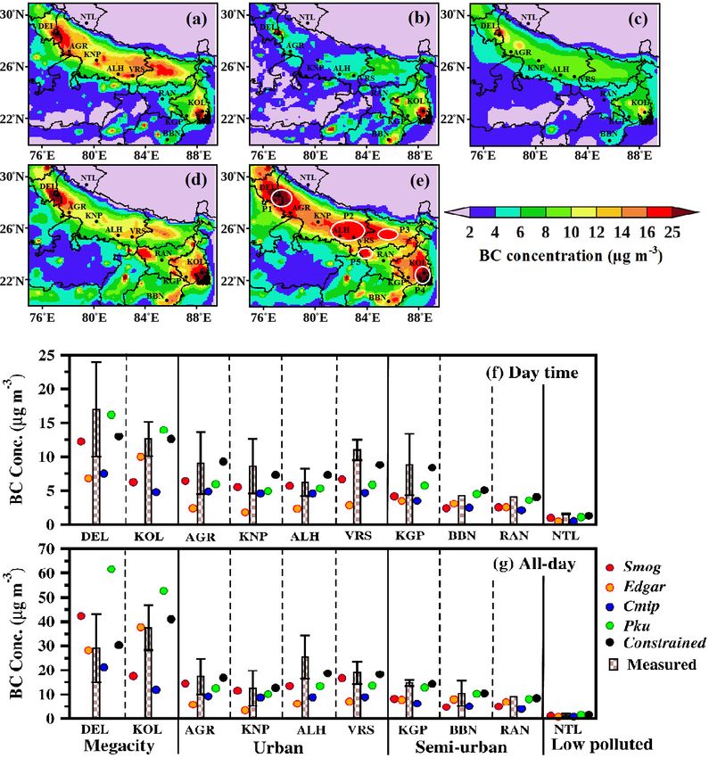
7674                                S. Ghosh et al.: Wintertime direct radiative effects of BC over the Indo-Gangetic Plain

Péré et al., 2011). Simulations are carried out at a horizon-      suring mass conservation for variables needing it. CHIMERE
tal grid resolution of 0.1◦ × 0.1◦ and over the domain span-       also reads anthropogenic emissions fields. Users can choose
ning from 20 to 30.8◦ N and 75 to 89.9◦ E, including the           the CHIMERE dedicated programme (called EMISURF; see
IGP region. BC transport simulations are performed for the         Menut et al., 2012) or make their own programme and create
winter of December 2015, keeping a spin-up time of 15 d in         a file on the CHIMERE grid directly.
November 2015 from 15 to 30 November. Evaluation of the
atmospheric BC concentration and BC-AOD in the present             2.1.2   The WRF meteorological model
study is done during the winter month of December when
the winter season is well developed in India and when the          The WRF model is a state-of-the-art numerical weather fore-
monthly mean BC concentration is typically observed as be-         cast and atmospheric simulation system designed for both re-
ing the highest (e.g. Pani and Verma, 2014). The simulation        search and operational applications. The initial and boundary
is done for the year 2015 as the recent bottom-up BC emis-         meteorological conditions for WRF simulations are obtained
sion database over India (Smog-India) implemented in the           from Global Forecast System (GFS) National Center for En-
present study is for the year 2015.                                vironmental Prediction FINAL operational global analysis
                                                                   data (NCEP-FNL, http://rda.ucar.edu/datasets/ds083.2/, last
2.1.1   The CHIMERE chemical transport model                       access: 15 June 2019) at a spatial resolution of 1◦ × 1◦ .
                                                                   Meteorological fields are simulated in WRF at the tempo-
CHIMERE is a regional chemical transport model designed            ral resolution of 1 h with the horizontal resolution the same
to model 10 gaseous species and aerosols. For chemistry, the       as that for the CHIMERE simulation. The meteorological
gaseous mechanism MELCHIOR2 is used (Derognat et al.,              boundary conditions are updated every 6 h. The optimised
2003). The calculation of aerosols is as described in Bessag-      schemes applied in the WRF simulation are as follows: Lin
net et al. (2004), with 10 bins and a mean mass-median dis-        scheme for cloud microphysics (Lin et al., 1983), Grell 3D
tribution ranging from 0.039 to 40 µm for primary particu-         ensemble scheme for subgrid convection (Grell and De-
late matter (black carbon – BC, organic carbon – OC, and           venyi, 2002), Yonsei University (YSU) scheme for boundary
PPMr – the remaining part of primary emissions), sulfate, ni-      layer (Hong et al., 2006), Rapid Radiative Transfer Model
trate, ammonium, sea salt, and water. Biogenic, dust, and sea      (RRTM) for radiation transfer (Mlawer et al., 1997), MM5
salt emissions are calculated online within CHIMERE. Bio-          Monin–Obukhov scheme for the surface layer, and Noah
genic emissions are estimated with the Model of Emissions          LSM for the land-surface model (Chen and Dudhia, 2001).
of Gases and Aerosols from Nature (Guenther et al., 2006).
Mineral dust and sea salt emissions are parameterised follow-      2.1.3   Implementation of BC emissions and multiple
ing Menut et al. (2015) and Monahan (1986), respectively.                  CHIMERE simulations
Secondary organic aerosols are formed following Bessag-
net et al. (2009). Chemical concentration fields are calcu-        In the present study, five simulations are carried out subjected
lated with a time step of a few minutes (using an adaptive         to the same model processes with CHIMERE but implement-
time step sensitive to the mean wind speed). For radiation         ing different BC emission inventories. The BC inventories
and photolysis, the online FastJX model is used (Wild et al.,      include recently estimated India-based (i) Constrainedemiss
2000). The horizontal transport is calculated with the Van-        and (ii) bottom-up BC emissions (Smog-India), as well as
Leer scheme (van Leer, 1979), and vertical transport is calcu-     bottom-up BC emissions from global datasets extracted over
lated using an upwind scheme with mass conservation from           India: (iii) EDGAR V4 (EDGAR), (iv) CMIP6, and (v) PKU.
Menut et al. (2013). Note that additional information is pro-      Spatially and temporally resolved gridded Constrainedemiss
vided in Table 1b. Boundary layer height is diagnosed us-          BC emissions over India are taken as per Verma et al. (2017).
ing the Troen and Mahrt (1986) scheme, and deep convec-            The observationally Constrainedemiss BC emissions or so-
tion fluxes are calculated using the Tiedtke (1989) scheme.        called Constrainedemiss BC emissions were estimated us-
Gaseous and aerosol species can be dry- or wet-deposited,          ing integrated forward and receptor modelling approaches
and fluxes are computed using the Wesely (1989) and Zhang          (Kumar et al., 2018; Verma et al., 2017). The estimation
et al. (2001) parameterisations. Initial and boundary condi-       was done by extracting information on initial bottom-up
tions are estimated using global model monthly climatol-           BC emissions and atmospheric BC concentration from the
ogy calculated with the Laboratoire de Météorologie Dy-            general circulation model (Laboratoire de Météorologie Dy-
namique General Circulation Model coupled with Interaction         namique atmospheric General Circulation Model – LMDZT-
with Chemistry and Aerosols (LMDz–INCA) (Szopa et al.,             GCM) simulation. The receptor modelling approach in-
2009). The domain grid has 20 vertical levels in σ -pressure       volved estimating the spatial distribution of potential emis-
coordinates ranging from the surface (997 hPa) to 200 hPa.         sion source fields of BC based on mapping the concentration-
CHIMERE reads the WRF hourly meteorological fields and             weighted trajectory (CWT) fields of measured BC (daytime
interpolates these meteorological fields if the CHIMERE grid       averaged) corresponding to the identified stations over the
is different. The interpolation is a bilinear interpolation, en-   Indian region. The Constrainedemiss BC emissions were ob-

Atmos. Chem. Phys., 21, 7671–7694, 2021                                              https://doi.org/10.5194/acp-21-7671-2021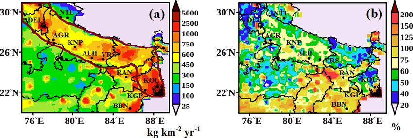
S. Ghosh et al.: Wintertime direct radiative effects of BC over the Indo-Gangetic Plain                                    7675

tained by modifying the initial or baseline bottom-up BC         try sector from the Constrainedemiss emission matches that
emissions of the GCM corresponding to the emission source        from bottom-up Smog-India relatively well. The seasonal-
fields of BC, thereby constraining the simulated BC concen-      ity in the spatial and temporal distribution of BC emission
tration in the GCM with the observed BC (refer to Verma          strength is inferred mainly from the open burning sector due
et al., 2017, for formulation and details).                      to the region- and season-specific prevalence of open burning
   A BC emission inventory based on the bottom-up ap-            of crop residues after harvesting of winter (rabi) and autumn
proach is generally compiled using information on activity       (kharif) crops, including forest biomass burning over the In-
data and generalised emission factors (see the references for    dian subcontinent (Venkataraman et al., 2006; Verma et al.,
bottom-up emissions, Table 1a). The recent bottom-up BC          2017). The BC emission flux is also noted as being the largest
emission database over India implemented is from Smog-           during winter months over the entire Indian subcontinent and
India (Pandey et al., 2014; Sadavarte and Venkataraman,          is specifically large over the IGP (Verma et al., 2017).
2014). The CMIP6 BC emissions used in the model simu-               Besides BC emissions, emissions of OC, SO2 , and PPMr
lations of CMIP6 are a combination of regional and global        are also implemented in CHIMERE. This implementation is
emission inventories re-gridded of EDGAR V4 (Eyring              done to perform atmospheric aerosol transport simulations
et al., 2016). In the present study, the global BC emis-         for the atmosphere with abundant aerosol species (including
sion inventories utilised include the emission databases for     BC) and for the atmosphere without BC. These simulations
EDGAR, CMIP6, and PKU re-gridded to the resolution               are required to calculate the radiative perturbations due to
as per the Smog-India database. The BC transport simula-         BC aerosol (refer to Sect. 2.3). The spatial distribution of the
tions in CHIMERE corresponding to the emission databases         mean and percentage standard deviation (δ as represented in
(Constrainedemiss , Smog-India, EDGAR, CMIP6, and PKU)           Eq. 4) of the BC emission flux from five BC emission inven-
are respectively referred to as the Constrained, Smog,           tories over the study domain is presented in Fig. 1a and b, re-
Edgar, Cmip, and Pku simulations. The annual BC emission         spectively. The mean BC emission flux is considerably high
strength over the study domain as estimated from the imple-      (450–1000 kg km−2 yr−1 ) over most of the IGP, with this be-
mented inventories lies in the range 415–1517 Gg yr−1 . De-      ing the highest (> 2500 kg km−2 yr−1 ) over the megacities
tails on the simulation experiment and a short description of    (Kolkata and Delhi). The divergence in the BC emission flux
BC emission inventories implemented are summarised in Ta-        is about 50 %–75 % over most of the IGP, with this being rel-
ble 1a. The classified source sectors of BC emission from the    atively lower over the eastern and upper mideastern IGP. The
emission inventory database include residential, open burn-      divergence is large in and around megacities (100 %–125 %)
ing, energy and industry, and transportation. The annual BC      and is noted to be specifically large (150 %–200 %) over rural
emission strength corresponding to each of the source sec-       locations in the lower mideastern IGP (in and around Palamu;
tors as available from the emission inventory database is also   refer to Fig. 3e for details on the location). Uncertainties in
mentioned in Table 1a. The fuel combustion activity among        activity data and emission factors have been inferred, lead-
the source sectors includes the following: the combustion        ing to uncertainty in bottom-up BC inventories greater than
of fuelwood, crop waste, dung cakes, kerosene, and cook-         200 % over India and Asia, as also mentioned earlier (Streets
ing liquified petroleum gas (LPG) for residential cooking        et al., 2003; Bond et al., 2004; Venkataraman et al., 2005;
and heating corresponding to the “residential” sector; open      Lu et al., 2011). One of the drawbacks of the bottom-up ap-
burning of agricultural residue, grassland, trash, and forest    proach is its inability to take into account possible unknown
biomass corresponding to the “open burning” source sector;       or missing emission sources. Bottom-up BC emissions are
coal and diesel for energy corresponding to the “energy and      thus found to often be lower than the actual emissions (Ryp-
industry” sector; and diesel, petrol, and gasoline correspond-   dal et al., 2005; Johnson et al., 2011; Zhang et al., 2005; Reid
ing to the “transportation” sector. Based on the available in-   et al., 2009). Bottom-up BC emissions over India include a
formation on sector-wise BC emission source strength (Ta-        large missing source of BC emitted over India (Venkatara-
ble 1a), the residential sector is seen to be the largest con-   man et al., 2006). Hence, the divergence in emission data
tributor to BC emissions over the Indian region, consistent      (refer Fig. 1b) using five emission datasets (observationally
with Venkataraman et al. (2005). The magnitude of annual         constrained and bottom-up BC emissions) is indicative of the
BC emission source strength corresponding to all the sec-        inadequacy of BC emission source strength, suggesting that
tors except the energy and industry sector is estimated to be    specific improvement is required in bottom-up BC emission
2 to 3 times larger for the Constrainedemiss emissions than      tabulation over the IGP and specific locations where the di-
the bottom-up emissions. This is specifically larger for the     vergence is typically noted to be large.
open burning sector, noted as 3 times the bottom-up Smog-
India emissions, thereby suggesting that specific improve-       2.2   Observational data for model evaluation and model
ment is required to quantify the BC emission strength of               sensitivity analysis
the open burning sector in the bottom-up BC emission in-
ventory. Interestingly, compared to the other source sectors,    The spatial distribution of WRF-simulated surface temper-
the BC emission source strength of the energy and indus-         ature over the IGP is compared with the available grid-

https://doi.org/10.5194/acp-21-7671-2021                                          Atmos. Chem. Phys., 21, 7671–7694, 2021
7676                                       S. Ghosh et al.: Wintertime direct radiative effects of BC over the Indo-Gangetic Plain

Table 1. Experimental set-up for the simulation of BC with CHIMERE.

  (a) Description of BC emission inventories implemented
  Name of       Emission            Domain          Annual BC emis-      Source sectors                 References
  the           (resolution)        (approach)      sion strength over   (emission
  simulation                                        study domain,        strength,
                                                    Gg yr−1              Gg yr−1 )
                                                    (base year)
  Smog          Smog-India          Indian          817                  Residential (393)              Sadavarte and Venkataraman (2014);
                (0.25◦ × 0.25◦ )    (bottom-up)     (2015)               Open burning (98)              Pandey et al. (2014);
                                                                         Energy and industry (163)      https://sites.google.com/view/smogindia
                                                                         Transportation (163)           (last access: 10 January 2020)
  Edgar         EDGAR               Global          579                  Residential (400)              Janssens-Maenhout et al. (2012);
                (0.1◦ × 0.1◦ )      (bottom-up)     (2010)               Energy and industry (127)      http://edgar.jrc.ec.europa.eu/ (last access: 9 July 2019)
                                                                         Transportation (52)
  Cmip          CMIP6               Global          558                  Anthropogenic (547)            Eyring et al. (2016);
                (0.5◦ × 0.5◦ )      (bottom-up)     (2014)               (residential, energy,          Feng et al. (2020);
                                                                         industry, commercial,          https://esgf-node.llnl.gov/projects/cmip6/
                                                                         transportation)                (last access: 11 November 2019)
                                                                         Open burning (11)
  Pku           PKU                 Global          415                  Residential                    Wang et al. (2014b);
                (0.1◦ × 0.1◦ )      (bottom-up)     (2007)               Open burning                   http://inventory.pku.edu.cn (last access: 9 July 2019)
                                                                         Energy and industry
                                                                         Transportation
  Constrained   Constrainedemiss    Indian          1517                 Residential (744)              Verma et al. (2017)
                (0.25◦ × 0.25◦ )    (constrained:   (latest)             Open burning (273)             http://www.facweb.iitkgp.ac.in/~shubhaverma/
                                    integrated                           Energy and industry (212)      constrained-bc-emissions-over-India.html
                                    receptor                             Transportation (288)           (last access: 2 August 2019)
                                    modelling
                                    with GCM)

                   (b) Details of the aerosol module in CHIMERE for BC (Menut et al., 2013)
                   Number of bins for BC    10 (mass-median diameter interval: 0.039, 0.078, 0.156, 0.312, 0.625, 1.25, 2.5, 5, 10, 20, 40 µm)
                   Aerosol mixing           Internal homogeneous
                   Aerosol dynamics         Absorption, nucleation, coagulation, ageing of BC
                   Deposition               Dry deposition and in-cloud or below-cloud wet deposition

Figure 1. Spatial distribution of (a) the mean and (b) percentage deviation (δ) of the BC emission flux from five BC emission inventories
implemented in CHIMERE over the study domain; the brown line in (a) indicates the IGP region.

ded distribution of observed temperature from the Climatic                         that observed from available measurements at stations over
Research Unit (CRU) (Morice et al., 2012). The observed                            the IGP (Table 2). The monthly mean simulated PBLH av-
temperature from the CRU at a horizontal resolution of                             erage is compared with that measured for available stations
0.5◦ × 0.5◦ is re-gridded to the same resolution (0.1◦ × 0.1◦ )                    in Delhi (mean of hourly PBLH during 10:00–16:00 LT),
as that from WRF, and the bias in simulated temperature for                        Kharagpur (10:00–11:00 and 14:00–15:00 LT), Ranchi (at
each grid cell is calculated using Eq. (1). The temporal trend                     14:30 LT), and Nainital (05:00–10:00 LT), corresponding to
of WRF-simulated hourly mean of meteorological parame-                             the overlapping time hours from measurements (Fig. 2l in
ters (temperature, relative humidity) is also evaluated with                       Sect. 3.1). The vertical distribution of the wintertime monthly

Atmos. Chem. Phys., 21, 7671–7694, 2021                                                                  https://doi.org/10.5194/acp-21-7671-2021
S. Ghosh et al.: Wintertime direct radiative effects of BC over the Indo-Gangetic Plain 7677
mean potential temperature (Stull, 1988) as obtained from 2013; Pani and Verma, 2014). Also, the daytime mean BC
WRF-simulated temperature is also compared with the mea- concentration exhibits low hourly variability and corresponds
sured vertical distribution of potential temperature for De- to the well-mixed layer of the atmosphere (Verma et al.,
cember (obtained for 2 d) at a station in Kanpur from an 2013; Pani and Verma, 2014). Hence, the lower value of the
available study (Table 2), corresponding to the overlapping daytime mean from the model than from observations is pri-
time hours (10:00–12:00 LT) from measurements. marily attributable to a low emission strength. Evaluation of
To compare the simulated BC surface concentration with model estimates for both the daytime and all-day mean thus
observations, the measured BC surface concentration is ob- provides a systematic hypothetical approach to identify the
tained at stations over the IGP from available studies (re- model discrepancy if primarily due to emissions or due to
fer to Table 2 and references therein). The selected sta- model processes attributed to meteorology (which is an input
tions correspond to area types identified as megacity (Delhi to the various aerosol processes that govern the atmospheric
and Kolkata), urban (Agra, Kanpur, Prayagraj – or Al- residence time of aerosols). This approach is further strength-
lahabad, and Varanasi), semi-urban (Kharagpur, Ranchi, ened by implementing BC emissions from five new BC emis-
and Bhubaneshwar), and low-polluted (Nainital). Comparing sion inventory databases and simulating BC transport sub-
model results with measurements thus aids in fulfilling the jected to the same aerosol physical and chemical processes
requirement to evaluate the model performance towards re- with CHIMERE.
producing the observed spatial patterns in BC distribution for Bias in simulated estimates (Xmodelled ) from simulations
the various area types. Measurement data used in the present at stations mentioned above for hourly, all-day, and daytime
study are reported with an uncertainty (due to instrument hours is estimated with respect to observed data (Xobs ) with
artefacts, etc.) of about 10 %–30 % for PBLH (Seidel et al., the equation as follows:
2010; Srivastava et al., 2010), 2 %–3 % for meteorological
parameters, and 5 %–20 % for the measured BC concentra- (Xmodelled − X obs )
Bias = × 100 %, (1)
tion (refer to Table 2 for details and references therein). It is Xobs
to be noted that observational data used for comparing model where X = BC concentration, temperature, relative humid-
estimates (meteorological parameters and BC aerosols) are ity, wind speed, and PBLH.
from measurements during different years at stations over Statistical analyses are carried out corresponding to day-
the IGP. The inter-annual variability of the PBLH (based time and all-day winter monthly mean to evaluate the nor-
on observations over Delhi) is reported as within 10 % (Iyer malised mean bias (NMB, Eq. 2) and root mean square error
and Raj, 2013), and for surface temperature (based on avail- (RMSE, Eq. 3) from the simulated results for N (N = 10 in
able measurement data from the India Meteorological De- this study) stations. We also evaluate the percentage devia-
partment over Kolkata and Kharagpur) it is less than 6 %. The tion (δ) in the simulated BC concentration attributed to BC
inter-annual variability of the atmospheric BC concentration emissions, estimated as the variability about the mean of the
over the Indian subcontinent is obtained as 5 %–10 % (Safai BC concentration from five simulations (refer to Eq. 4).
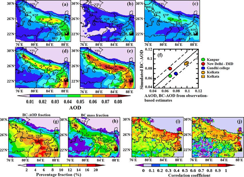
et al., 2014; Surendran et al., 2013; Bisht et al., 2015; Ram Further, the BC-AOD estimated in the present study (re-
et al., 2010b; Kanawade et al., 2014; Pani and Verma, 2014). fer to Sect. 2.3) is compared with aerosol absorption optical
This is taking into account that the reported inter-annual vari- depth (AAOD) from Aerosol Robotic Network (AERONET;
ability of meteorological parameters and the atmospheric BC level: 2) measurements over the IGP (Giles et al., 2012; Hol-
concentration is nearly equivalent to or within the uncertainty ben et al., 1998) at stations in Kanpur, at New Delhi IMD, at
range for measurements and is also much lower than the dis- Gandhi College (25.87◦ N, 84.12◦ E), and at the IIT Kharag-
crepancy between simulated and observed BC as reported in pur extension in Kolkata. The wintertime AAODs avail-
previous studies (refer to Sect. 1). The uncertainty range is able from AERONET observations for Kanpur, New Delhi
taken into consideration while evaluating the model perfor- IMD, Gandhi College (December 2010–2015 averaged), and
mance compared to measurements. The comparison between Kolkata (February 2009 averaged) are used in the compari-
model estimates and measurements at widespread geograph- son. For Kolkata, the comparison is also made with the es-
ical locations and area types as presented in this study is timated BC-AOD for the December 2010 period as obtained
therefore justified and is primarily required for evaluating the from the configured aerosol model using in situ ground-based
model performance and enhancing the statistical analysis. observations for the same period (Verma et al., 2013). The
The model-estimated and measured BC concentrations are AERONET AAOD data are available at four wavelengths:
compared corresponding to daytime (10:00–16:00 LT) and 440, 675, 870, and 1020 nm. The AAOD at the wavelength
all-day (24-hourly) winter monthly mean values. This com- of 550 nm (used for comparison with simulated BC-AOD in
parison is made because measured BC concentrations are the present study) is obtained based on the wavelength de-
found to exhibit a strong diurnal variability, with a rela- pendence of AAOD as per Giles et al. (2012).
tively lower value during daytime hours than during the late A correlation study is also carried out between the variance
evening to early morning hours; this is attributed to pre- of emissions and simulated BC concentrations or simulated
vailing wintertime meteorological conditions (Verma et al., BC-AOD from the simulations to examine the sensitivity of
https://doi.org/10.5194/acp-21-7671-2021 Atmos. Chem. Phys., 21, 7671–7694, 20217678 S. Ghosh et al.: Wintertime direct radiative effects of BC over the Indo-Gangetic Plain
the simulated BC concentration or BC-AOD to the variation logical initial and boundary conditions provided to the model
in emission magnitude. are as per the WRF model, as mentioned previously (refer to
Sect. 2.1.2). The Rapid Radiative Transfer Model for GCMs
N
scheme (RRTM-G) (Iacono et al., 2008) is selected for short-
BCmodelled − BCobs
P
1 wave and longwave radiation. The direct and diffused com-
NMB = × 100 % (2) ponents of solar irradiance are separately addressed with the
N
BCobs
P
RRTM-G scheme to improve the model calculations by con-
1 sidering surface irradiance components in the estimation.
# 21
Simulations for radiative flux with WRF-Solar are per-
"
N
1 X
RMSE = (BCmodelled − BCobs )2 (3) formed for each of the three cases, as mentioned above, using
N 1
respective simulated optical properties as input for each case.
σ The shortwave (SW) radiative flux (at 550 nm) for clear-sky
δ= × 100 % (4)
mean conditions is estimated at the top (TOA) and bottom (SUR)
Here, σ is the standard deviation for the mean from five sim- layer of the atmosphere for the atmosphere with BC and
ulations (e.g. BC emissions, all-day, daytime mean of BC without BC. This is done by subtracting the respective flux
concentration). at TOA and SUR due to wAero from the flux due to wBC
and BCaero, respectively. The direct radiative perturbations
2.3 Simulation of wintertime BC-AOD and radiative or the direct radiative effects (DREs) due to BC aerosols at
perturbations due to BC over the IGP TOA (DRETOA (BC)) and at SUR (DRESUR (BC)) are calcu-
lated by taking the difference between the radiative flux from
The BC-AOD is estimated with OPTical properties SIM- BCaero and that from wBC at the respective layers of the at-
ulation (OPTSIM) (Stromatas et al., 2012) using the mosphere (Eqs. 5 and 6). The DRE in the atmosphere (ATM)
three-dimensional BC mass concentration obtained from due to BC is estimated by subtracting the flux at the SUR
CHIMERE corresponding to each of the five simulations from that estimated at TOA (Eq. 7).
(refer to Table 1). Aerosol optical properties are estimated
based on Mie theory calculations considering internal mix- DRETOA (BC) = [DRETOA (BCaero) − DRETOA (wAero)]
ing (Lesins et al., 2002; Permadi et al., 2018b). These esti- − [DRETOA (wBC) − DRETOA (wAero)] (5)
mations are done at six wavelengths of 440, 500, 532, 550,
870, and 1064 nm and the same horizontal and temporal res- DRESUR (BC) = [DRESUR (BCaero) − DRESUR (wAero)]
olution as of CHIMERE. − [DRESUR (wBC) − DRESUR (wAero)] (6)
For radiative transfer calculations, estimates from the Con- DRE ATM
(BC) = DRETOA (BC) − DRESUR (BC) (7)
strained simulation (which is determined to be the most ef-
ficient to simulate the BC distribution, as discussed later)
and the Smog simulation (from India-based BC emissions as 3 Results and discussion
a representative bottomup simulation) are only considered.
For estimating the radiative effect due to BC aerosols, simu- 3.1 Analysis of WRF-simulated meteorological
lation of aerosol optical properties (AOD, single-scattering parameters
albedo – SSA, and the Ångström exponent – AE) is con-
ducted with OPTSIM for three different cases considering The WRF-simulated winter monthly mean distribution of the
(i) the atmosphere including BC (with BC, BCaero), (ii) the horizontal wind speed, vertical wind velocity, and PBLH
atmosphere without BC (without BC, wBC), and (iii) the over the IGP are presented in Fig. 2a–c. As observed from
atmosphere with no aerosol (without aerosol, wAero). The the wind field distribution map, there is a predominance of
three-dimensional aerosol species concentration as an in- weak north-easterlies (1–2 m s−1 ) over the IGP. The vertical
put to OPTSIM is derived for each of the three cases from wind velocity distribution indicates a neutral air mass or a
CHIMERE corresponding to the simulations (Constrained downdraft of the air mass over the IGP (a positive value of
and Smog simulations). the vertical wind velocity is an indication of a downdraft of
Aerosol radiative transfer calculations are done in WRF- the air mass and vice versa). The presence of a narrow PBLH
Solar at a temporal resolution of 1 h and horizontal grid (200 to 600 m) over most of the IGP indicates low vertical
resolution of 0.1◦ × 0.1◦ by selecting a regular longitude– mixing during winter (Fig. 2c). The topographical elevation
latitude projection. The WRF Preprocessing System (WPS) decreases from the northern IGP towards the eastern IGP,
internally converts the grid resolution corresponding to with the maximum elevation observed on the northward side
longitude–latitude projection from degrees to metres as re- due to the Himalayan mountains (Fig. 2d).
quired for model processing. WRF-Solar is a new version of A high load of BC aerosols over the IGP as obtained (dis-
the WRF model enhanced for the prediction of solar irradi- cussed later) in the present study is inferred due to confine-
ance (Haupt et al., 2016; Jimenez et al., 2016). The meteoro- ment of pollution near the surface within the shallow bound-
Atmos. Chem. Phys., 21, 7671–7694, 2021 https://doi.org/10.5194/acp-21-7671-2021S. Ghosh et al.: Wintertime direct radiative effects of BC over the Indo-Gangetic Plain 7679
Table 2. Observational data used for model validation from available studies at identified locations over the study domain.
Type Stations Location Data (year of References
measurement)
Megacity Delhi (DEL) 28.58◦ N, 77.20◦ E BC conc. (2004) Ganguly et al. (2006)
PBLH (2006) Bano et al. (2011)
AAOD (2011–2015) https://aeronet.gsfc.nasa.gov
(last access: 7 May 2020)
Kolkata (KOL) 22.54◦ N, 88.42◦ E BC conc., temp., RH, Pani and Verma (2014);
wind speed (2011–2014) Research group, IIT-KGP
AAOD (2009) https://aeronet.gsfc.nasa.gov
BC-AOD (2009–2011) (last access: 7 May 2020)
Verma et al. (2013)
Urban Agra (AGR) 27.20◦ N, 78.10◦ E BC conc. (2004) Safai et al. (2008)
Kanpur (KNP) 26.51◦ N, 80.23◦ E BC conc. (2007) Ram et al. (2010a)
Vertical profile of Tripathi et al. (2005b)
potential temp. (2004) https://aeronet.gsfc.nasa.gov
AAOD (2011–2015) (last access: 7 May 2020)
Gandhi College 25.87◦ N, 84.12◦ E AAOD (2013) https://aeronet.gsfc.nasa.gov
(last access: 7 May 2020)
Prayagraj–Allahabad (ALH) 25.41◦ N, 81.91◦ E BC conc. (2004) Badarinath et al. (2007)
Varanasi (VRS) 25.30◦ N, 83.00◦ E BC conc. (2009) Singh et al. (2015)
Semi- Kharagpur (KGP) 22.19◦ N, 87.19◦ E BC conc., temp., RH, Priyadharshini (2019);
urban wind speed (2011–14) Research group, IIT-KGP
PBLH (2004) Nair et al. (2007)
Bhubaneshwar (BBN) 20.50◦ N, 85.5◦ E BC conc. (2010–2011) Mahapatra et al. (2014)
Ranchi (RAN) 23.50◦ N, 85.30◦ E BC conc. (2010) Lipi and Kumar (2014)
PBLH (2011) Chandra et al. (2014)
Low- Nainital (NTL) 29.37◦ N, 79.45◦ E BC conc. (2004–2007) Dumka et al. (2010)
polluted PBLH (2011) Singh et al. (2016)
ary layer height in winter due to low vertical mixing and large (about ± 10 % to ± 25 %) over a few grids in the north-
weak dispersion of atmospheric pollutants. This creates stag- eastern, western, and southern IGP. A comparative study of
nant weather under the prevailing meteorological conditions, the hourly distribution of the winter monthly mean simu-
with low temperature, weak wind speed, the downdraft of lated surface temperature and relative humidity (RH), with
the air mass, and a narrow PBLH (as presented above). In the corresponding observed value from available measure-
addition, the Himalayan mountains northward further inhibit ments at Kharagpur (semi-urban) and Kolkata (megacity),
the dispersion of aerosol pollutants and favour their confine- is presented in Fig. 2h–k. Please refer to Table 2 for de-
ment over the IGP. This inference is also in corroboration tails on observational data. The temporal trend of the simu-
with observational studies at stations over the IGP (e.g. Nair lated hourly winter monthly mean of meteorological param-
et al., 2007, 2012; Pani and Verma, 2014; Verma et al., 2014; eters conforms to the measurements. The magnitude of the
Vaishya et al., 2017; Rana et al., 2019). Further, the IGP also hourly distribution of the winter monthly mean surface tem-
comprises the highest population density and therefore en- perature from simulations (Fig. 2h and j) is found to com-
hanced BC emission strength during winter, specifically from pare well with that from observations during daytime hours
biofuel combustion, e.g. fuelwood and crop waste for resi- (10:00–16:00 LT) for both stations; it is, however, seen to be
dential cooking and heating (Venkataraman et al., 2005; Sahu underestimated (bias: −45 % to −58 %) during midnight to
et al., 2015; Verma et al., 2017; Rana et al., 2019). early morning hours (00:00–05:00 LT). The WRF-simulated
We compare the spatial distribution of monthly mean tem- meteorology is input to various aerosol processes that gov-
perature from WRF simulations (Fig. 2e) with that from grid- ern the atmospheric residence time of aerosols in CHIMERE
ded ground-based observations from CRU (Fig. 2f). The bias and thereby influences the atmospheric concentration of BC
in model-estimated temperature is found to be within ± 5 % aerosols. A lower value of simulated surface temperature
over most of the IGP (Fig. 2g) but is noticed to be slightly than observed during midnight to early morning hours would
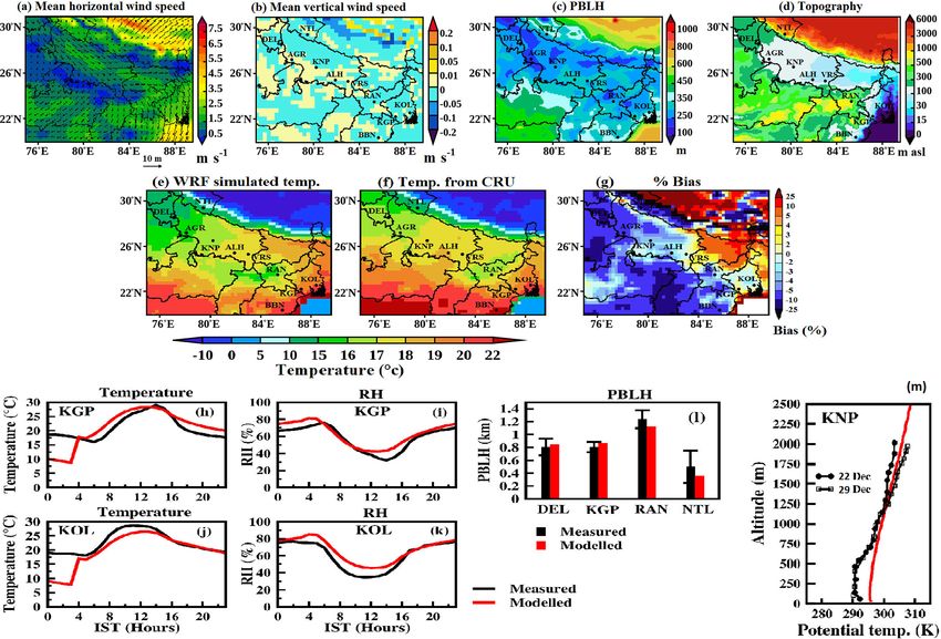
https://doi.org/10.5194/acp-21-7671-2021 Atmos. Chem. Phys., 21, 7671–7694, 20217680 S. Ghosh et al.: Wintertime direct radiative effects of BC over the Indo-Gangetic Plain Figure 2. Spatial distribution of the WRF-simulated (a–c) winter monthly mean (a) horizontal wind field (note that the colour scale is for wind speed in m s−1 and the arrows indicate the direction of the mean field), (b) vertical wind speed at 1000 hPa, (c) planetary boundary layer height (PBLH in metres), and (d) topography (metres above sea level, m a.s.l.) (e–g) Spatial distribution of winter monthly mean surface temperature from (e) WRF simulations, (f) observations from CRU, and (g) percentage bias in WRF estimates. (h–k) Comparison of the hourly distribution of winter monthly mean (h, j) surface temperature and (i, k) relative humidity from WRF simulations with observations at stations (Kharagpur, KGP; Kolkata, KOL). (l) Comparison of winter monthly mean PBLH during day hours between measured and simulated values at the stations under study. The error bars represent the standard deviation (σ ) in the measured PBLH. (m) Comparison of the vertical profile of potential temperature obtained from WRF (winter monthly mean) and measurements (2 d). lead to decreased mixing of pollutants, enhancing their ac- ±10 %) at all stations. Although at Nainital the simulated cumulation in the atmosphere during these hours (as also bias is large (−28 %), it is within the range of uncertainty evinced in the diurnal distribution of the simulated BC con- in observations as mentioned in Sect. 2.2. The vertical pro- centration; refer to Sect. 3.2, Fig. 4). file of potential temperature (Fig. 2m) from WRF (winter- The WRF-simulated RH at both stations (Fig. 2i and k) time monthly mean) resembles that measured at a station in is in good agreement with measurements (bias: −5 % to Kanpur, with the bias being less than 4 % up to the height of +35 %), with the mean RH during late evening to early 500 m and less than 1 % at a higher altitude (> 500 m). morning hours (20:00–05:00 LT) being 2 times higher than Thus, the WRF-simulated winter monthly mean of the me- that during daytime. A comparison of winter monthly mean teorological parameters, including their temporal trend, con- PBLH during daytime hours (as described in Sect. 2.2) forms well with the observations. However, it is required to from the WRF simulation with that available from observa- reduce the discrepancy, specifically in the simulated magni- tions at Delhi, Kharagpur, Ranchi, and Nainital is also pre- tude of temperature during midnight to early morning hours. sented (Fig. 2l). The standard deviations (1σ ) in measured A better temporally resolved meteorological boundary con- PBLH values are within 10 %–16 % for Delhi, Kharagpur, dition in WRF (compared to 6-hourly from NCEP in the and Ranchi and about 49 % at Nainital. The simulated PBLH present study), aided by data assimilation at a fine temporal is close enough to measurements (bias estimated within resolution (e.g. 1-hourly) using diurnal meteorological ob- Atmos. Chem. Phys., 21, 7671–7694, 2021 https://doi.org/10.5194/acp-21-7671-2021
S. Ghosh et al.: Wintertime direct radiative effects of BC over the Indo-Gangetic Plain 7681
servations for India-based stations, would potentially lead to The simulated spatial pattern in the Constrained simula-
more accurate simulation of the observed magnitude of the tion is consistent with observations (Fig. 3f–g), as the BC
diurnal distribution of meteorological parameters; an assess- distribution features for the specific area types are repre-
ment in this regard is required in a future study. sented well by the simulated BC distribution. The spatial fea-
ture also indicates that the wintertime all-day mean value
3.2 Simulated wintertime BC concentration with new of the BC concentration (Fig. 3g) in Delhi is lower than
BC emissions as modelled with CHIMERE: impact Kolkata and vice versa for the daytime mean value (Fig. 3f),
of changing emissions and comparison with although the BC emission strength (refer to Fig. 1a) of the
measurements two megacities, Delhi and Kolkata, is nearly equivalent. We
discuss these features in context with the transport of BC
The spatial distribution of the winter monthly mean BC aerosols over the IGP based on the visualisation of an an-
surface concentration from five simulations over the IGP imation (https://doi.org/10.5446/48819; Ghosh and Verma,
is shown in Fig. 3a–e. The simulated mean BC concentra- 2020) later in the section. The simulated magnitude of the
tion from the Constrained simulation is, in general, 2 to BC surface concentration from the Constrained simulation,
4 times higher than that derived from the bottomup simu- compared to that from the bottomup simulations, resembles
lation over most of the IGP. Five hotspots or patches (re- the measured counterpart relatively well (Fig. 3f–g), with the
fer to Fig. 3e) with a large BC concentration (magnitude ratio of the measured to simulated all-day (daytime) mean
> 16 µg m−3 ) from the Constrained simulation are identified BC concentration being equivalent to nearly 1. A detailed
in and around megacities (Delhi and Kolkata), in surrounding statistical analysis of the comparison between simulated and
semi-urban areas, in urban spots over the central (Prayagraj– observed BC is presented later in this section.
Allahabad–Varanasi) and mideastern IGP (Patna), and in one The mean and standard deviation of the simulated BC con-
rural spot over the lower mideastern IGP (Palamu). It is in- centration from five simulations at stations under study are
teresting to see that the hotspots observed in the Constrained provided in Table 3a (also refer to Fig. 4). Analysis of multi-
simulation are also identified in the Pku simulation, mostly simulations indicates that the percentage deviation (δ, refer
in the Smog simulation as well, though with a smaller value to Eq. 4) in the simulated BC concentration (Table 3a) at-
than the Constrained simulation. Estimates from the Edgar tributed to emissions is specifically the lowest for the low-
and Cmip simulations simulate the megacity hotspots but fail polluted location (e.g. Nainital) and is generally within 40 %
to show the other identified hotspots in the Constrained sim- for all other locations under study. The δ for the megacity
ulation. Interestingly, the hotspot at Palamu (a coal-mining is noted as being typically more amplified (51 %–56 %) dur-
belt in Jharkhand) is simulated in the Constrained and Pku ing the late evening to early morning hours (Table 3a, Fig. 4)
simulations, unlike the rest of other simulations, thereby sug- than during daytime hours (35 %–43 %) compared to other
gesting a lack of BC emission source strength corresponding locations under study. This suggests that under similar me-
to Palamu and other identified hotspot locations in bottom-up teorological conditions and with the same aerosol processes
BC emissions (as also mentioned in Sect. 2.1.3). The simu- in the model, the deviation in the simulated BC concentra-
lated spatial pattern (refer to Fig. 3f–g) of the BC surface tion can be attributed to emissions increases from daytime to
concentration in the Constrained simulation, while exhibiting late evening hours, thus indicating that increased emissions
the lowest value at high-altitude and low-polluted locations potentially amplify the accumulation of BC pollutants and
(e.g. Nainital), moderately high values at semi-urban stations worsen air quality over megacities, specifically during the
(e.g. Kharagpur and Ranchi), and high values at urban sta- late evening to morning hours compared to daytime hours,
tions (e.g. Agra, Kanpur, Allahabad–Prayagraj, Varanasi), is raising concern for megacity commuters.
seen to reach a maximum in megacities (Kolkata and Delhi). On comparing the temporal distribution of the simulated
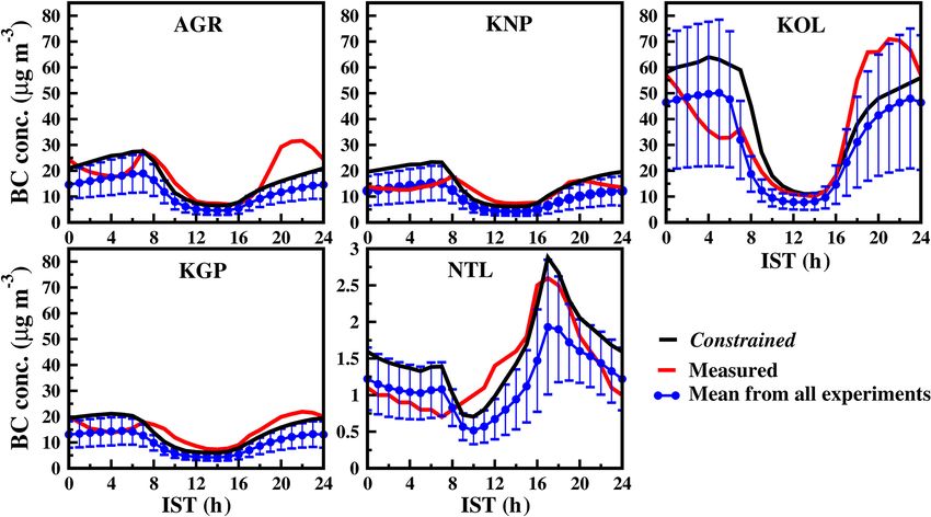
In comparison to the Constrained simulation, the simulated BC concentration from the Constrained simulation with that
spatial gradient within and across the area types is seen to of the measured concentration, it is seen that the pattern of
be inconsistent in bottomup simulation estimates. For exam- simulated diurnal variability (shown for selected stations; re-
ple, the bottomup estimated values of the BC concentration fer to Fig. 4) is consistent with that measured. The diur-
from the Smog and Cmip simulations have a low spatial gra- nal variability of the BC concentration is relatively higher,
dient from the megacity (Kolkata) to urban area type, includ- by a factor of 2 to 5, in the Constrained simulation during
ing a lack of spatial contrast compared to the observations the late evening to early morning hours (20:00–05:00 LT)
among the urban stations; the Pku simulation overestimates than during daytime hours (10:00–16:00 LT) at all stations
the all-day mean BC concentration for megacities but simu- (except Nainital). Notably, this factor is equivalent to that
lates the spatial gradient relatively well across the area types. obtained from the bottomup simulations and also to that
The Edgar simulation matches the observed values well in from observations (Surendran et al., 2013; Pani and Verma,
megacities for the all-day mean but then underestimates the 2014; Ram and Sarin, 2010; Nair et al., 2012; Dumka et al.,
observations by a large value and with a low spatial contrast 2010; Lipi and Kumar, 2014). The diurnal variability in the
among the urban and semi-urban stations. BC surface concentration is mainly associated with the at-
https://doi.org/10.5194/acp-21-7671-2021 Atmos. Chem. Phys., 21, 7671–7694, 2021You can also read