Simulating age of air and the distribution of SF6 in the stratosphere with the SILAM model
←
→
Page content transcription
If your browser does not render page correctly, please read the page content below
Atmos. Chem. Phys., 20, 5837–5859, 2020
https://doi.org/10.5194/acp-20-5837-2020
© Author(s) 2020. This work is distributed under
the Creative Commons Attribution 4.0 License.

Simulating age of air and the distribution of SF6 in the stratosphere
with the SILAM model
Rostislav Kouznetsov1,2 , Mikhail Sofiev1 , Julius Vira1 , and Gabriele Stiller3
1 Finnish Meteorological Institute, Helsinki, Finland
2 Obukhov  Institute for Atmospheric Physics, Moscow, Russia
3 Karlsruhe Institute of Technology, Karlsruhe, Germany

Correspondence: Rostislav Kouznetsov (rostislav.kouznetsov@fmi.fi)

Received: 27 June 2019 – Discussion started: 4 July 2019
Revised: 26 March 2020 – Accepted: 8 April 2020 – Published: 15 May 2020

Abstract. The paper presents a comparative study of age of        1   Introduction
air (AoA) derived from several approaches: a widely used
passive-tracer accumulation method, the SF6 accumulation,         The age of air (AoA) is defined as the time spent by an air
and a direct calculation of an ideal-age tracer. The simula-      parcel in the stratosphere since its entry across the tropopause
tions were performed with the Eulerian chemistry transport        (Li and Waugh, 1999; Waugh and Hall, 2002). The distribu-
model SILAM driven with the ERA-Interim reanalysis for            tion of the AoA is controlled by the global atmospheric circu-
1980–2018.                                                        lations, primarily the Brewer–Dobson and polar circulations.
   The Eulerian environment allowed for simultaneous appli-       In particular, the temporal variation of AoA has been used
cation of several approaches within the same simulation and       as an indicator of the long-term changes in the stratospheric
interpretation of the obtained differences. A series of sensi-    circulation (Engel et al., 2009; Waugh, 2009). AoA has been
tivity simulations revealed the role of the vertical profile of   extensively used for evaluation and comparison of general
turbulent diffusion in the stratosphere, destruction of SF6 in    circulation and chemical transport models in the stratosphere
the mesosphere, and the effect of gravitational separation of     (Waugh and Hall, 2002; Engel et al., 2009).
gases with strongly different molar masses.                          Simulations of the AoA as defined above have been per-
   The simulations reproduced well the main features of the       formed with Lagrangian transport models. The trajectories
SF6 distribution in the atmosphere observed by the MIPAS          are initiated with positions distributed in the stratosphere and
(Michelson Interferometer for Passive Atmospheric Sound-          integrated backwards in time until they cross the tropopause.
ing) satellite instrument. It was shown that the apparent very    The time elapsed since the initialization is attributed as age
old air in the upper stratosphere derived from the SF6 pro-       of air at the point of initialization. Moreover, the distribution
file observations is a result of destruction and gravitational    of the ages of particles originating from some location can be
separation of this gas in the upper stratosphere and the meso-    used to get the age spectrum there. Until recently, Lagrangian
sphere. These processes make the apparent SF6 AoA in the          simulations of AoA did not explicitly account for turbulent
stratosphere several years older than the ideal-age AoA,          mixing in the stratosphere (Eluszkiewicz et al., 2000; Waugh
which, according to our calculations, does not exceed 6–6.5       and Hall, 2002; Diallo et al., 2012; Monge-Sanz et al., 2012).
years. The destruction of SF6 and the varying rate of emis-       Accounting for mixing adds up to 2 years to the mean AoA
sion make SF6 unsuitable for reliably deriving AoA or its         in the tropical upper stratosphere (Garny et al., 2014). In La-
trends. However, observations of SF6 provide a very use-          grangian models, the mixing can be simulated with random-
ful dataset for validation of the stratospheric circulation in    walk of the particles (Garny et al., 2014) or by inter-parcel
a model with the properly implemented SF6 loss.                   mixing (Plöger et al., 2015; Brinkop and Jöckel, 2019).
                                                                     The Eulerian simulations of AoA can be formulated in
                                                                  several ways. The approaches with an accumulating tracer,
                                                                  whose mixing ratio increases linearly in the troposphere,

Published by Copernicus Publications on behalf of the European Geosciences Union.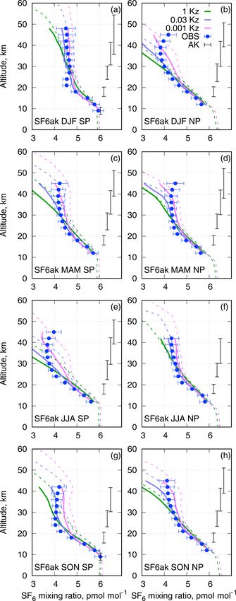
5838                                                                                 R. Kouznetsov et al.: Modelling age of air

were used in a comprehensive study by Krol et al. (2018)            assumptions behind these methods. For a similar problem
and several studies before (e.g. Eluszkiewicz et al., 2000;         with the ages of oceanic water, it has been shown (Waugh
Monge-Sanz et al., 2012). Another approach is to simulate a         et al., 2003) that, in the case of a inhomogeneously growing
steady distribution of a decaying tracer, such as 221 Rn, emit-     tracer, the tracer age is strongly influenced by the shape of
ted at the surface at a constant rate (Krol et al., 2018). Be-      the transient time distribution (TTD, also known as the “age
sides that, a special tracer that is analogous to the Lagrangian    spectrum”) at the particular location and time.
clock has been used. The tracer appears in the literature under        Another major source of uncertainty in the observational
names such as “clock-type tracer” (Monge-Sanz et al., 2012)         AoA is the violation of conservation of the tracer due to
or “ideal age” (Waugh and Hall, 2002). The ideal age has a          sources and sinks, such as oxidation of carbon monoxide and
constant rate of increasing of mixing ratio everywhere, ex-         methane for CO2 or mesospheric destruction for SF6 . The
cept for the surface where it is continuously forced to zero.       mesospheric sink of SF6 leads to “over-ageing”, especially
Similar tracers have long been used to simulate the trans-          pronounced in the area of the polar vortices. The magnitude
port times of oceanic water (e.g. England, 1995; Thiele and         of the over-ageing was estimated to be as at least 2 years
Sarmiento, 1990).                                                   (Waugh and Hall, 2002). Besides being visible in many eval-
   Direct observations of the age of air, as it is defined above,   uations, e.g. Stiller et al. (2012, Fig. 4) and Kovács et al.
are not possible; therefore, AoA is usually derived from the        (2017, Fig. 8), the over-ageing of the polar winter strato-
observed mixing ratios of various tracers with known tro-           spheric air was studied by Ray et al. (2017, Fig. 4) within
pospheric mixing ratios and lifetimes (Bhandari et al., 1966;       the dedicated exercise.
Koch and Rind, 1998; Jacob et al., 1997; Patra et al., 2011) or        The simulations of SF6 and the AoA in the atmosphere
from the long-living tracers with known variations in the tro-      with the WACCM model (Kovács et al., 2017) have also
pospheric mixing ratios. The studies published to date used         reproduced the effect of over-ageing. However, its magni-
carbon dioxide (CO2 ; Andrews et al., 2001; Engel et al.,           tude was much smaller than that inferred from the SF6 re-
2009), nitrous oxide (N2 O; Boering et al., 1996; Andrews           trievals of the limb-viewing MIPAS (Michelson Interferom-
et al., 2001), sulfur hexafluoride (SF6 ; Waugh, 2009; Stiller      eter for Passive Atmospheric Sounding) instrument operated
et al., 2012), methane (CH4 ; Andrews et al., 2001; Remsberg,       on board of the Envisat satellite in 2002–2012 (Stiller et al.,
2015), and various fluorocarbons (Leedham Elvidge et al.,           2012) and from the in situ observations of the ER-2 aircraft
2018).                                                              (Hall et al., 1999). Kovács et al. (2017) offered two possi-
   For accumulating tracers, the mean AoA at some point in          ble reasons for the discrepancy: either SF6 loss is still under-
the stratosphere is calculated as a lag between the times when      estimated in WACCM or MIPAS SF6 observations are low
a certain mixing ratio is observed near the surface and at that     biased above ∼ 20 km. Neither of the cases have been anal-
point. The lag time is equivalent to the mean AoA defined           ysed in depth, which leaves the status of MIPAS, currently
above only in the case of the strictly linear growth and the        the richest observational dataset for the stratospheric SF6 ,
uniform distribution of the tracer in the troposphere (Hall and     unclear.
Plumb, 1994).                                                          The aim of the present study is to provide self-consistent
   In reality, there is no tracer whose mixing ratio in the         simulations of the spatio-temporal distribution of the AoA
troposphere grows strictly linearly. The violation of the as-       and of the SF6 mixing ratio in the troposphere and the strato-
sumption of the linear growth leads to biases in the resulting      sphere during the last 39 years. The main modelling tool
AoA distribution and its trends. It has been pointed out that       is the Eulerian chemistry transport model SILAM (System
the increasing growth rates of CO2 and SF6 lead to a low            for Integrated modeLling of Atmospheric coMposition). The
bias of AoA and its trends and make these tracers ambigu-           stratospheric balloon observations and retrievals of the limb-
ous proxies of the AoA (Garcia et al., 2011). Various correc-       viewing MIPAS instrument mentioned above are used for
tions have been applied in several studies (Hall and Plumb,         validation of the simulated distribution.
1994; Waugh and Hall, 2002; Engel et al., 2009; Stiller et al.,        With these simulations we
2012; Leedham Elvidge et al., 2018) to deduce the “true”
AoA from observations of tracers with the increasing growth           – compare different methods of estimating the AoA and
rates. The effect of the correction method on the AoA es-               quantify the inconsistencies in the AoA and its trends
timates has not been investigated and must be considered a              arising from violations of the underlying assumptions
source of uncertainty in the resulting estimates. Thus, Gar-            behind each method,
cia et al. (2011) concluded that accounting for the biases in         – analyse the causes of the discrepancies in the upper
the trend estimates due to varying growth rates would likely            stratosphere between different methods of deriving the
require uniform and continuous knowledge of the evolution               AoA,
of the trace species, which is not available from any exist-
ing observational dataset. Recently Leedham Elvidge et al.            – provide a solid basis for further studies of stratospheric
(2018) showed a minor sensitivity of the AoA to the choice              circulation with observations of various trace gases and
of the correction method but without detailed analysis of the           for studies of climate effects of SF6 .

Atmos. Chem. Phys., 20, 5837–5859, 2020                                               https://doi.org/10.5194/acp-20-5837-2020
R. Kouznetsov et al.: Modelling age of air                                                                                  5839

   The paper is organized as follows. Section 2 gives an           The SILAM configuration, used for the present study, is de-
overview of the modelling tools and the modelling and obser-       scribed in Sect. 3.4.
vational data used for the study. Section 3 describes the de-
velopments made for SILAM in order to perform the simula-          2.2   ECMWF ERA-Interim reanalysis
tions: vertical eddy-diffusivity parameterization in the strato-
sphere and the lower mesosphere and the SF6 destruction            The ERA-Interim reanalysis of the European Centre for
parametrization, as well as the model configuration used for       Medium-Range Weather Forecasts (ECMWF) had been used
the study. The sensitivity tests and evaluation of the simula-     as a meteorological driver for our simulations. The dataset
tions against the MIPAS retrievals and stratospheric balloon       has T255 spectral resolution and covers the whole atmo-
measurements of SF6 mixing ratios are given in Sect. 4. Sen-       sphere with 60 hybrid sigma-pressure levels having the up-
sitivity of the AoA and its trends to the simulation setup and     permost layer from 0.2 to 0 hPa with nominal pressure of
the choice of particular SF6 tracer as an AoA proxy is stud-       0.2 hPa (Dee et al., 2011). The reanalysis uses a 12 h data as-
ied in Sect. 5. The uncertainties of the used modelling ap-        similation cycle, and the forecasts are stored with a 3 h time
proach and implications of AoA derived from SF6 tracer are         step. We used the fields retrieved from the ECMWF’s MARS
discussed in Sect. 6. The results are summarized in Sect. 7.       archive on a long–lat grid, 500 × 250 points, with a step of
                                                                   0.72◦ . The four forecast times (+3, +6, +9 and +12 h) were
                                                                   used from every assimilation cycle to obtain a continuous
                                                                   dataset with 3 h time step. To drive the dispersion model,
2     Methods and input data                                       the data on horizontal winds, temperature, and humidity for
                                                                   1980–2018 were used.
2.1    SILAM model                                                    Since the resolution of the driving meteorology was twice
                                                                   higher than that of SILAM, the meteorological input for both
SILAM (System for Integrated modeLling of Atmospheric              cell interface for winds and cell mid-points for other parame-
coMposition, http://silam.fmi.fi, last access: 13 May 2020)        ters (surface pressure, temperature, and humidity) was avail-
is an offline 3D chemical transport model. SILAM features          able without interpolation. The gridded ERA-Interim fields
a mass-conservative positive-definite advection scheme that        are, however, a result of reprojection of the original mete-
makes the model suitable for long-term runs (Sofiev et al.,        orological fields computed as spherical harmonics. More-
2015). The model can be run at a range of resolutions starting     over, the difference in the topmost layer of the ERA-Interim
from a kilometre scale in a limited-area up to a global cover-     and SILAM data required vertical reprojection at the top of
age. The vertical structure of the modelling domain consists       the domain. Together with the limited precision of the grid-
of stacked layers starting from the surface. The layers can        ded fields retrieved from the ECMWF archive, they caused
be defined either in z- or hybrid sigma-pressure coordinates.      some inconsistency between the surface-pressure tendencies
The model can be driven with a variety of NWP (numerical           and the vertically integrated air-mass fluxes calculated from
weather prediction) or climate models.                             the meteorological fields in SILAM. Albeit small, such in-
   The global 3D simulations of atmospheric transport for a        consistencies cause spurious variations in wind-field diver-
variety of tracers representing AoA and SF6 (see Sect. 3.4         gence that might result in gradual accumulation of errors in
for details) were performed with SILAM for the years 1980–         the tracer mixing ratios. To maintain strict global and local
2018 with the global long–lat grid of 1.44◦ × 1.44◦ cells          air-mass budget throughout the run, the wind fields were ad-
(250 × 123 grid cells plus polar closures) and 60 hybrid           justed by distributing the residuals of pressure tendency and
sigma-pressure layers starting from the surface. The up-           vertically integrated horizontal air-mass fluxes as a correc-
permost layer was between pressures of 0.1 and 0.2 hPa,            tion to the horizontal winds, as suggested by Heimann and
whereas other layer bounds corresponded to the half levels         Keeling (1989). The correction was, at most, of the order of
of the meteorological driver – the ERA-Interim reanalysis          centimetres per second, which is comparable to the preci-
(Sect. 2.2). The model time step was 15 min and the output         sion of the input wind fields. The vertical wind component
consisted of daily-mean 3D concentrations of the tracers and       was then rediagnosed from the divergence of the horizontal
air density. Emission data were taken from the SF6 emission        air-mass fluxes for the SILAM layers as described in Sofiev
inventory (Rigby et al., 2010), which was extrapolated un-         et al. (2015). Validity of this procedure was demonstrated by
til 2016 as described in Sect. 3.4. Physical–chemical trans-       its authors Heimann and Keeling (1989) and its applicability
formations of the SF6 -related tracers required developments       to the current case was confirmed in the Sect. 5.2 by compar-
described in Sect. 3.3.                                            ison with another model simulations driven by ERA-Interim
   In order to accurately model the AoA and the needed trac-       (Diallo et al., 2012).
ers, the vertical diffusion part of the transport scheme of           The ERA-Interim reanalysis has been used earlier for La-
SILAM has been refined to account for gravitational sepa-          grangian simulations of AoA (Diallo et al., 2012) and has
ration. In addition, several tracers with corresponding trans-     been found to provide ages that agree with those inferred
formation routines have been implemented into the model.           from in situ observations in the lower stratosphere.

https://doi.org/10.5194/acp-20-5837-2020                                            Atmos. Chem. Phys., 20, 5837–5859, 2020
5840                                                                                    R. Kouznetsov et al.: Modelling age of air

2.3    MIPAS observations of SF6

To evaluate the results of the SF6 modelling, we used the
data from the MIPAS instrument operated on board Envisat
in 2002–2012. MIPAS is a limb-sounding Fourier transform
spectrometer with a high spectral resolution measuring in
the infrared part of spectrum. Due to its limb geometry,
the instrument provided good vertical resolution of the de-
rived trace-gas profiles and showed high sensitivity to low-
abundance species around the tangent point. Along the or-
bit path, MIPAS measured a profile of atmospheric radiances
about every 400 km with an altitude coverage, in its nominal
mode, from 6 to 70 km. The vertical sampling was 1.5 km
in the lower part of the stratosphere (up to 32 km) and 3 km
above, with a vertical field of view covering 3 km at the tan-
gent point. Over a day, about 1300 profiles along 14.4 orbits
were measured, covering all latitudes up to the poles at sunlit
and dark conditions. The vertical distributions of trace gases
were derived from the radiance profiles by an inversion pro-
cedure, fitting simulated spectra to the measured ones while          Figure 1. Vertical profiles of diffusion coefficients are shown. The
varying the atmospheric state parameters.                             distribution of the ERA5 profiles of the “mean turbulent diffusion
   The retrieval of SF6 is based on the spectral signature of         coefficient for heat” parameter, molecular diffusivity for SF6 in the
this species in the vicinity of 10.55 µm wavelength and is de-        U.S. Standard Atmosphere, and the three prescribed Kz profiles are
scribed in Stiller et al. (2008), Stiller et al. (2012), and Haenel   shown. The eddy diffusion profile due to breaking gravity waves
et al. (2015). In the current study, we use an updated version        (after Lindzen, 1981) is given for the reference.
of the SF6 data (compared to the one described in Haenel
et al., 2015) called V5H/R_SF6_21/224/225. The new algo-
                                                                      3     SILAM developments
rithm uses the new absorption cross-section data on the SF6
and a new CFC-11 band in the vicinity of the SF6 signature            Destruction of atmospheric SF6 occurs at altitudes above
by Harrison (2018) instead of the older cross-section data by         60 km (Totterdill et al., 2015) that fall within the topmost
Varanasi et al. (1994). The updated version provides up to            layer of the ERA-Interim data. The exchange processes in
0.6 pmol mol−1 higher SF6 mixing ratios in the upper part             the upper stratosphere and lower mesosphere have to be ade-
of the stratosphere (above 30 km) than the old versions and           quately parameterized together with the destruction process.
is closer to independent reference data. Note that whilst we          In our simulations we have suppressed the transport of SF6
regard this newer version of MIPAS SF6 data as an improve-            with mean wind through the modelling domain top (0.1 hPa,
ment, it has not yet been reported in a publication, and on           65 km) and parameterized the SF6 loss due to the eddy and
that basis it is subject to uncertainty.                              molecular diffusion towards the altitudes where the destruc-
   The retrieved profiles are sampled on an altitude grid             tion occurs. In this section we introduce the set of parameter-
spaced at 1 km, whereas the actual resolution of the profiles         izations that were implemented in SILAM for this study.
is between 4 and 10 km for altitudes below 30 km. The re-
trievals are supplemented with averaging kernels and error            3.1    Eddy diffusivity
covariance matrices describing the uncertainties due to ran-
dom noise in the radiance measurements, hereinafter referred          A large variety of vertical profiles for eddy diffusivity in the
to as measurement noise error, target noise error, or retrieval       stratosphere and the lower mesosphere can be found in litera-
noise error. This error component, which is normally of the           ture. In many studies in the 1970s–1980s, the vertical profiles
order of 10 % of the retrieved value, is fully uncorrelated           were derived from observed tracer concentrations neglecting
from profile to profile, and therefore it virtually cancels out       the mean transport. Most studies suggested that the vertical
when averaged over a large number of profiles. In contrast,           eddy diffusion has a minimum of 0.2–0.5 m2 s−1 (Pisso and
there exist systematic error components that are fully corre-         Legras, 2008) at 15–20 km, agreeing quite well to the ones
lated between the profiles. Their assessment is difficult and         derived from the radar measurements in the range of 15–
depends on the knowledge about sources of systematic er-              20 km (Wilson, 2004). Above that altitude, Kz was suggested
rors. Stiller et al. (2008) has assessed them to be of the order      to gradually increase by about 1.5 orders of magnitude to-
of 10 % at 60 km and 4 % at 30 km. These error components             wards 50 km due to breaking gravity waves (Lindzen, 1981).
have to be considered when comparisons of monthly or sea-                The theoretical estimates of the effective exchange coeffi-
sonal means with other data are performed.                            cients, considering the layered and patchy structure of strato-

Atmos. Chem. Phys., 20, 5837–5859, 2020                                                  https://doi.org/10.5194/acp-20-5837-2020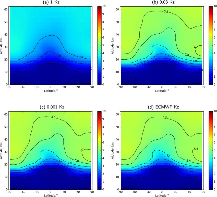
R. Kouznetsov et al.: Modelling age of air 5841
spheric turbulence, suggest 0.5–2.5 m2 s−1 for the upper tro- the SILAM Kz to the prescribed one occurs in the altitude
posphere and 0.015–0.02 m2 s−1 for the lower stratosphere range of 10–15 km.
(Osman et al., 2016), which is about an order of magnitude
lower than the estimates above. 3.2 Molecular diffusivity and gravitational separation
The values of the eddy exchange coefficient at heights
of 10–20 km estimated from the high-resolution balloon In tropospheric and stratospheric chemistry transport mod-
temperature measurements (Gavrilov et al., 2005) are ∼ els (CTMs), gaseous admixtures are transported as tracers
0.01 m2 s−1 with no noticeable vertical variation. It is not (i.e. advection and turbulent mixing do not depend on the
clear, however, how representative the derived values are for species properties), whereas the molecular diffusion is neg-
UTLS (upper troposphere and lower stratosphere) in general. ligible. Models that cover the mesosphere, such as WACCM
We could not find any reliable observations of vertical diffu- (Smith et al., 2011), account for molecular diffusion explic-
sion in a range of 30–50 km. itly. Since some of the Kz parameterizations of the previous
The parameterization for vertical eddy diffusivity above section often result in values below the molecular diffusivity,
the boundary layer used in SILAM has been adapted from the parametrization of molecular diffusion has been imple-
the IFS model of the European Centre for Medium-Range mented in SILAM.
Weather Forecasts (ECMWF, 2015). However, in the upper The molecular diffusivity of SF6 in the air at tem-
troposphere the predicted eddy diffusivity is nearly zero. For perature T0 = 300 K and pressure p0 = 1000 hPa is D0 =
numerical reasons, a lower limit of 0.01 m2 s−1 is set for Kz 10−5 m2 s−1 (Marrero and Mason, 1972, Table 22). The dif-
in SILAM. Our sensitivity tests have shown that long-term fusivity at different temperature T and pressure p is given
simulations are insensitive to this limit as long as it is low by
enough. The Kz in the stratosphere is routinely set to the
p0 T 3/2
limiting value with relatively rare peaks, mostly in UTLS. D = D0 , (2)
Such a scheme essentially turns off turbulent diffusion in the p T0
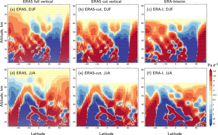
stratosphere. The same is true for the recent ERA5 reanalysis (e.g. Cussler, 1997). The vertical profile of molecular diffu-
dataset (Copernicus Climate Change Service , C3S) that pro- sivity in the U.S. Standard Atmosphere (NOAA et al., 1976)
vides the values of Kz among other model-level fields: the is shown in (Fig. 1). Note that the value for the reference dif-
eddy diffusion routinely falls below the molecular diffusivity fusivity of SF6 used in this paper is about a half of the one
above 40 km (Fig. 1). used in simulations with WACCM by Kovács et al. (2017).
As a reference for this study, we took a tabulated profile The reason is that WACCM uses a universal parametrization
of Hunten (1975), as it was quoted by Massie and Hunten (Smith et al., 2011, Eq. 7 there) for all compounds. That
(1981). The original profile covers the range up to 50 km, parametrization relies solely on molecular mass of a tracer
and the extrapolation up to 80 km matches the theoretical es- and does not account for, for example, the molecule collision
timates by Lindzen (1981) and by Allen et al. (1981). We radius. The latter is about twice larger for SF6 than for most
approximate the profile as a function of pressure in the range of stratospheric tracers. Thus, for this study we use the value
of 100–0.01 hPa (15–60 km): from Marrero and Mason (1972), which results from fitting
0.75 laboratory data for diffusion of SF6 in the air.
1 hPa The vertical diffusion transport velocity of admixture with
Kz (p) = 8 m2 s−1 . (1)
p number concentration ñ and molecular mass µ̃ in neutrally
stratified media is given by Mange (1957):
The approximated profile was stitched with the default
SILAM profile with a gradual transition within an altitude 1 ∂ µ̃ µ̃ µg
w = −D + −1 , (3)
range of 10–15 km to keep the tropospheric dispersion in- µ̃ ∂z µ kT
tact. This profile gives values of Kz 3–6 orders of magni-
tude higher than the ones provided by the ERA5 reanalysis where µ is molecular mass of air, g is acceleration due to
(Fig. 1) and 1–2 orders of magnitude higher than the esti- gravity, k is the Boltzmann constant, and T is temperature.
mates of Legras et al. (2005). With the ideal gas law p = nkT , in which p is pressure and
In order to cover the range of Kz values between the ERA5 n is number concentration, and the static law dp/dz = −gρ,
profiles and the reference one (Eq. 1), we used two inter- where ρ = µn is air density, Eq. (3) can be reformulated in
mediate profiles obtained by scaling the reference one with terms of admixture mixing ratio ξ = ñ/n and pressure. Then
factors 0.03 and 0.001. The three prescribed eddy-diffusivity the vertical gradient of the equilibrium mixing ratio will be
profiles are hereinafter referred to as “1-Kz”, “0.03-Kz”, ∂ξ
µ̃
ξ
and “0.001-Kz”, respectively. The dynamic eddy-diffusivity = −1 . (4)
∂p µ p
profile adopted from the ECMWF IFS is referred to as
“ECMWF-Kz”. In all simulations, the parameterization of It is non-zero for an admixture of a molecular mass different
Kz in the troposphere is the same, and linear transition from from the one of air. Integrating the gradient Eq. (4) over the
https://doi.org/10.5194/acp-20-5837-2020 Atmos. Chem. Phys., 20, 5837–5859, 2020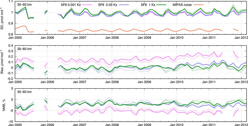
5842                                                                                 R. Kouznetsov et al.: Modelling age of air

vertical, one can find that the equilibrium mixing ratios ξ1
and ξ2 at two levels with corresponding pressures p1 and p2
are related as
       µ̃/µ−1
ξ1       p1
   =               .                                     (5)
ξ2       p2
For heavy admixtures, such as SF6 (µ̃ = 0.146 kg mol−1 ) the
equilibrium gradient of a mixing ratio is substantial. For ex-
ample, the difference of the equilibrium mixing ratio of SF6
between 0.1 and 0.2 hPa is a factor of 16.
   In most of the atmosphere, the effect of gravitational sepa-
ration is insignificant due to the overwhelming effect of other
mixing mechanisms, whereas in the upper stratosphere the
molecular diffusivity may become significant. Therefore, in
the upper stratosphere heavy gases can no longer be consid-
ered tracers and the molecular diffusion should be treated ex-
plicitly. The effect of gravitational separation of nitrogen and
oxygen isotopes in the stratosphere has been observed (Ishi-
doya et al., 2008, 2013; Sugawara et al., 2018); however, for
isotopes the ratio of masses is relatively small, so the ob-       Figure 2. The vertical profiles of SF6 destruction rate (after Totter-
                                                                   dill et al., 2015) and its approximation in the range of 55–75 km,
served differences were also small (up to 10−5 ). For SF6 , the
                                                                   given by Eq. (6).
molecular mass difference is much larger.
   In order to enable the gravitational separation in SILAM,
we have introduced the molecular diffusion mechanism,              resolve the vertical structure of the atmosphere above that
which can be enabled along with the turbulent diffusion            level. In order to assess the loss of SF6 , we have to param-
scheme. The exchange coefficients due to molecular diffu-          eterize the combined effect of the SF6 transport through the
sion between the model layers are precalculated according to       0.1 hPa and its destruction. Then the resulting fluxes can be
Eq. (3) and discretized for the given layer structure for each     applied as the upper boundary condition for our simulations.
species according to its diffusivity and molar mass. The U.S.         As an approximation to the vertical profile of the destruc-
Standard Atmosphere (NOAA et al., 1976) was assumed for            tion rate in an altitude range of 50–80 km, we have fitted the
the vertical profiles of temperature and air density during pre-   corresponding part of the curve in Fig. 9a of Totterdill et al.
calculation of the exchange coefficients. The exchange has         (2015) with a power function of pressure (magenta line in
been applied throughout the domain at every model time step        Fig. 2):
with a simple explicit scheme.
                                                                                          0.2 hPa 3

                                                                    1
3.3    SF6 destruction                                                = 3 × 10⁻⁸ s−1                ,                         (6)
                                                                   τ                         p
Estimates of AoA from the SF6 tracer rely on the assump-           where τ is the lifetime of SF6 at the altitude corresponding
tion of it being a passive tracer. SF6 is indeed essentially       to pressure p.
stable in the troposphere and the stratosphere. IPCC (2013,           The topmost level of the ERA-Interim meteorological
Sect. 8.2.3.5) mentions that photolysis in the stratosphere as     dataset is located at 0.1 hPa, which is below the layer where
the main mechanism of SF6 loss but without any reference to        the destruction of SF6 occurs. Therefore, we have to put a
original studies. The statement is probably taken from Rav-        boundary condition on our simulations to account for the up-
ishankara et al. (1993). Reddmann et al. (2001) pointed at         ward flux of SF6 through the upper boundary of the simu-
associative electron attachment in the upper stratosphere and      lation domain. For that, we assume that the SF6 distribution
mesosphere as the main destruction mechanism for SF6 be-           above the computational domain top is in equilibrium with
low 80 km. The recent study of Totterdill et al. (2015) gives      the destruction and the vertical flux.
some 1–2 orders of magnitude slower rates of electron at-             Assuming the profiles for Kz (p) and the SF6 lifetime τ (p)
tachment but keeps it the dominant mechanism of the SF6            are given by Eqs. (1) and (6), one can obtain a steady-state
destruction in the altitude range up to 100 km. The highest        distribution of the mass-mixing ratio, ξ , of SF6 due to de-
destruction rate of 10−5 s−1 occurs at the altitude of 80 km       struction in the mesosphere at any point where both Eqs. (1)
(Fig. 2). An important feature of this profile is that the de-     and (6) are valid and vertical advection is negligible. The lat-
struction rate becomes significant above the top of our mod-       ter assumption implies that the diffusive vertical flux over-
elling domain (0.1 hPa, 65 km). The ERA-Interim meteoro-           whelms the advective one. The validity and implications of
logical fields have the uppermost level at 0.1 hPa and do not      neglecting the regular vertical transport are discussed below.

Atmos. Chem. Phys., 20, 5837–5859, 2020                                               https://doi.org/10.5194/acp-20-5837-2020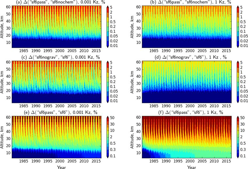
R. Kouznetsov et al.: Modelling age of air                                                                                     5843

                                                                      F (p)/ξ(p) gives an equivalent regular vertical air-mass flux
                                                                      that would result in the same vertical flux of SF6 if it were
                                                                      passive and non-diffusive. The equivalent regular vertical ve-
                                                                      locity ωeq (in units of the Lagrangian tendency of a parcel
                                                                      pressure due to vertical advection) can be expressed as
                                                                      ωeq = −gF (p)/ξ(p).                                       (10)
                                                                         Accounting for molecular diffusion may either enhance or
                                                                      reduce the upward flux of SF6 in the model. Along with set-
                                                                      ting the equilibrium state with the bulk of a heavy admixture
                                                                      being in the lower layers, molecular diffusion provides addi-
                                                                      tional means for transport to the upper layers where the de-
                                                                      struction occurs. For very low eddy diffusivities, the molec-
                                                                      ular diffusion is a sole mechanism of the upward transport
                                                                      of SF6 towards depletion layers. For higher eddy diffusivity,
Figure 3. Vertical profiles of steady-state upward flux of SF6 nor-   the effect of molecular diffusion and gravitational separation
malized with mass mixing ratio, F (p)/ξ(p), for eddy-diffusivity      becomes negligible.
and lifetime profiles given by Eqs. (1) and (6). The topmost model       For the model consisting of stacked well-mixed finite lay-
layer of SILAM and effective lifetimes of SF6 there due to the de-    ers, the loss of SF6 from the topmost layer due to the steady
struction in the mesosphere for different Kz profiles are given.      upward flux would be proportional to the SF6 mixing ratio in
                                                                      the layer. This loss of mass is equivalent to a linear decay of
                                                                      SF6 in the layer at a rate
The steady-state profile of ξ can be obtained from a solution
of the steady-state diffusion equation with a sink:                               F (p)
                                                                      τ −1 = g          ,                                       (11)
                                                                                 ξ(p)1p
∂ξ     ∂        ξ
   = g (F ) −       = 0,                                       (7)    where 1p is pressure drop in the layer.
∂t    ∂p      τ (p)
                                                                         In the upper layer of our simulations (between 0.1 and
where ρ(p) is air density, g is acceleration due to gravity,          0.2 hPa, grey rectangle in Fig. 3), the SF6 lifetime τ due
and the upward flux of SF6 is given by                                to turbulent diffusion is about 3 d for Kz of Eq. (1). After
                                                                      scaling the Kz (p) profile with factors of 0.03 and 0.001, one
                      ∂ξ
F (p) = gρ 2 Kz (p)      .                                     (8)    gets the lifetimes of 15 and 60 d, respectively. Note that the
                      ∂p                                              molecular diffusion sets the upper limit to the SF6 lifetime
   The above equation was solved numerically as a bound-              in the topmost model layer: it can not be longer than 60 d
ary value problem with unit mixing ratio at a height of 1 hPa         for the 0.1–0.2 hPa layer. Close to this regime, the system
and vanishing flux, F (p) at p = 0, for the set of Kz pro-            becomes insensitive to the actual profile and values of the
files. The shooting method with bisection was used to get             turbulent diffusion coefficient. The loss of SF6 through the
the steady-state profiles of ξ(p) and F (p), corresponding            domain top was implemented as a linear decay of SF6 in the
to ξ(1 hPa) = 1. For all considered cases, the flux F (p) de-         topmost model layer, at a rate corresponding to the Kz (p)
creased by several orders of magnitude already at the level of        profile used in each simulation.
a few pascals (Pa), i.e. below the maximum of the depletion
                                                                      3.4   Simulated tracers
profile of Totterdill et al. (2015), indicating that the particular
shape of τ (p) above that level does not influence the fluxes         SILAM performs the 3D transport by means of a dimension
at the domain top (0.1 hPa). The steady-state upward flux of          split: transport along each dimension is performed separately
SF6 F (p) normalized with the corresponding mixing ratio at           as 1D transport. To minimize the inconsistency between the
each pressure, F (p)/ξ(p), for the three test profiles of Kz is       tracer transport and air-mass fluxes caused by the dimension
shown in Fig. 3 with solid lines.                                     split at finite time step, the splitting sequence has been in-
   The gravitational separation can be accounted for by in-           verted at each time step. The residual inconsistency was re-
troducing a term responsible for molecular diffusion and its          solved by using a separate unity tracer, which was initialized
equilibrium state Eq. (4) into the vertical flux Eq. (8) :            to the constant mass mixing ratio of 1 at the beginning of a
                      ∂ξ

                                         ∂ξ µ̃ − µ ξ
                                                                     simulation. Should advection be perfect, the concentration of
            2                   2
F (p) = gρ Kz (p)         + gρ D(p)          −              . (9)     the unity tracer would be equivalent to air density (mixing ra-
                      ∂p                 ∂p       µ p
                                                                      tio would stay equal to 1). The mixing ratios of the simulated
The profiles of F (p)/ξ(p) resulting from F (p) in Eq. (7)            tracers were then evaluated as a ratio of the tracer mass in a
are given in Fig. 3 with dashed lines. The magnitude of               cell to the mass of the unity tracer.

https://doi.org/10.5194/acp-20-5837-2020                                               Atmos. Chem. Phys., 20, 5837–5859, 2020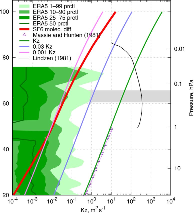
5844                                                                                 R. Kouznetsov et al.: Modelling age of air

   In order to assess the effects of gravitational separation and   4     Sensitivity and validation of SF6 simulations
destruction on the atmospheric distribution of SF6 , we used
four tracers: SF6 as a passive tracer sf6pass, SF6 with grav-       4.1    Gravitational separation and mesospheric
itational separation but no destruction sf6nochem (no chem-                depletion
istry), SF6 with destruction but no gravitational separation
sf6nograv, and SF6 with both gravitational separation and           To evaluate the relative importance of gravitational separa-
destruction in the upper model level sf6.                           tion, mesospheric depletion, and their effect on the SF6 con-
   All SF6 tracers had the same emission according to the SF6       centrations, we compared the simulations for the SF6 tracers
emission inventory (Rigby et al., 2010). The inventory cov-         and evaluated the relative reduction of the SF6 content in the
ers 1970–2008 and was extrapolated with a linearly grow-            stratosphere due to these processes. As a conservative esti-
ing trend of 0.294 Gg yr−2 until July 2016. The last 2.5            mate of the reduction, we evaluated the relative differences
years were run without the SF6 emissions to evaluate its            between the tracers in the latitude belt of 70–85◦ S, since
destruction rate. Note that the emission extrapolation gives        both processes have the most pronounced effect in the south-
9.4 Gg yr−1 for 2016, which is somewhat higher than the             ern polar vortex, where the downwelling of Brewer–Dobson
later estimate of 8.8 Gg yr−1 (Engel et al., 2018).                 circulation is the strongest.
   Besides the four SF6 tracers, we used a passive tracer emit-        Hereafter we quantify the relative difference between at-
ted uniformly at the surface at constant rate during the whole      mospheric contents of two SF6 tracers, “X” and “Y” as
simulation time and an ideal-age tracer. The ideal-age tracer                          ξX − ξY
is defined as a tracer whose mixing ratio ξia obeys the conti-      1(“X”, “Y”) = 2            · 100 %.                          (14)
                                                                                       ξX + ξY
nuity equation (Waugh and Hall, 2002)
                                                                    The relative differences for the SF6 tracers in the southern
∂ξia
     + L(ξia ) = 1                                          (12)    polar region (70–85◦ S) simulated with two extreme Kz pro-
 ∂t                                                                 files is given in Fig. 4 as a function of time and altitude. Note
(where L is the advection–diffusion operator), and boundary         that every 5 % of the decrease of SF6 with respect to its pas-
condition ξia = 0 at the surface. The ideal-age tracer is trans-    sive counterpart corresponds to about 1 year of a positive bias
ported as a regular gaseous tracer and updated at every model       in AoA derived from the SF6 mixing ratios.
time step 1t with the unity tracer correction:                         The reduction of the SF6 content due to gravitational sep-
                                                                   aration, if the mesospheric depletion is disabled, is given by
             0,                 at lowest layer,
Mia 7 −→                                                    (13)    the relative difference of sf6nochem and sf6pass (Fig. 4a,
             Mia + Munity 1t otherwise,
                                                                    b). Expectedly, the effect of gravitational separation is most
where Mia and Munity are masses of the ideal-age tracer and         pronounced for the case of low eddy diffusivity (0.001-Kz),
of the unity tracer in the grid cell. The mixing ratio of the       and the reduction of SF6 in the altitude range of 30–50 km
ideal-age tracer is a direct measure of the mean age of air         reaches 2 %–5 %. In the case of strong mixing, the effect of
in a cell, so the tracer is a direct Eulerian analogue of the       separation is about 1 %.
time-tagged Lagrangian particles with clock reset at the sur-          The reduction of the SF6 content due to gravitational sep-
face. Note that the AoA derived from the ideal-age tracer           aration in the presence of stratospheric depletion is given by
and AoA from a passive tracer with a linearly growing near-         the relative difference of sf6nograv and sf6 tracers. The ef-
surface mixing ratio are equivalent (Waugh and Hall, 2002),         fect of the separation for low Kz is very similar between the
and implementation of both provides a redundancy needed to          depletion and no-depletion cases (Fig. 4c vs. Fig. 4a). Deple-
ensure self-consistency of our results.                             tion reduces the effect of the gravitational separation for high
   The simulations were performed with four eddy-                   Kz (Fig. 4b vs. Fig. 4d). Regardless of depletion, stronger Kz
diffusivity profiles described in Sect. 3.1 and the correspond-     reduces the effect of the gravitational separation; however,
ing destruction rates of sf6 and sf6nograv tracers in the up-       the latter is still non-negligible if precisions of the order of a
permost model layer. All runs were initialized with the mix-        month for AoA are required.
ing ratios from the final state of a special initialization run.       The combined effect of depletion and gravitational separa-
The initialization simulation with 0.1-Kz eddy diffusivity          tion is seen in the relative difference of sf6pass and sf6 tracers
was started from 1970 with zero fields for all tracers, except      (Fig. 4e and f). For both Kz cases, the effect of depletion is
for the unity tracer that was set to unity mixing ratio. The        stronger than the diffusive separation by more than 1 order
simulation used 1970–1989 emissions for SF6 species from            of magnitude. Regardless of the Kz profiles, the reduction
the same inventory as for the main runs (Rigby et al., 2010),       exceeds 50 %, which roughly corresponds to 10 years of an
and it was driven with the twice repeated ERA-Interim me-           offset in the apparent AoA.
teorological fields for 1980–1989. The mixing ratios of all            In all cases the reduction of the SF6 content has a strong
SF6 tracers at the end of the initialization run were scaled to     annual cycle associated with the cycle of the downwelling in
match the total SF6 burden of 20.17 Gg in 1980 (Levin et al.,       winter and the upwelling in summer. Besides, the reduction
2010).                                                              has a noticeable inter-annual variability that poses substan-

Atmos. Chem. Phys., 20, 5837–5859, 2020                                               https://doi.org/10.5194/acp-20-5837-2020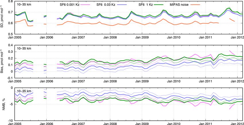
R. Kouznetsov et al.: Modelling age of air 5845
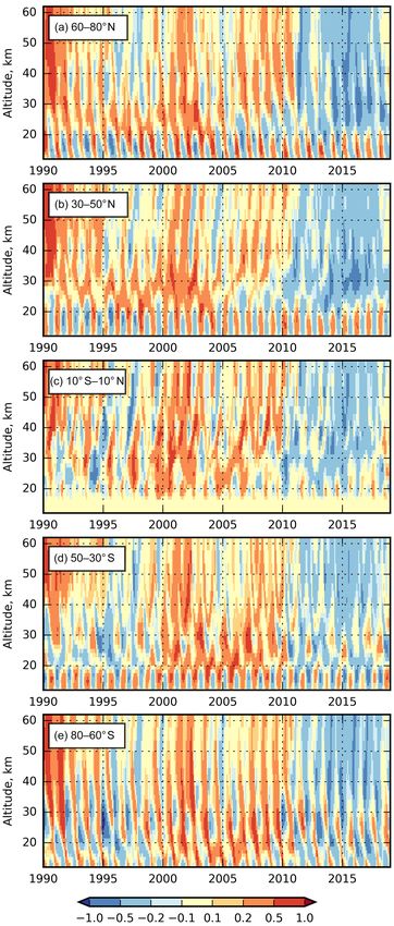
Figure 4. The relative reduction of the SF6 content (in %) at 70–85◦ S due to gravitational separation with (a, b) and without (c, d) depletion
and due to the combined effect of depletion and separation (e, f) at two extreme Kz cases. Note the different colour scales for (e) and (f).
tial difficulties for applying a consistent correction to the ap- eddy-diffusivity profiles in the stratosphere. The difference
parent AoA. Contrary to the former two comparisons, strong in the modelled profiles can, however, be seen above the
eddy mixing leads to a strong reduction of SF6 since it inten- tropopause. For comparison, we took the simulations with
sifies the transport to the depletion layers and thus enhances prescribed eddy diffusivity in the stratosphere (1-Kz, 0.03-
the depletion rate. Kz, and 0.001-Kz; see Sect. 3.1) and with dynamic eddy
The simulations for different Kz have been initialized with diffusivity ECMWF-Kz. The simulations were matched with
the same state obtained from a separate spin-up simulation the stratospheric balloon observations (Fig. 5) published by
with 0.01-Kz, which was scaled to match total burden of SF6 Patra et al. (1997), Engel et al. (2006), Ray et al. (2014), and
in 1980. Thus a relaxation of the SF6 vertical distribution Ray et al. (2017).
during the first few years of the simulations is clearly seen Two balloon profiles observed at Hyderabad (17.5◦ N,
in Fig. 4. For the 1-Kz case (Fig. 4f), the gradual increase 78.6◦ E) in 1987 and 1994 by Patra et al. (1997) indicate
of the difference between SF6 and its passive version in the an increase of the SF6 content during the time between the
troposphere can be seen as well. The rate of this increase is soundings (Fig. 5a). Both profiles have a clear transition layer
about 0.5 % per 39 years of the simulations. This rate should from tropopause at ∼ 17 km to the undisturbed upper strato-
not be confused with the depletion rate of SF6 in the atmo- sphere above ∼ 25 km. The simulated profiles agree quite
sphere since the difference is a combined effect of depletion well with the observed profiles, except for the most diffusive
and growth of emission rate, despite the fact that the latter is case that gave notably smoother profiles and somewhat over-
exactly the same for both tracers. stated SF6 mixing ratios due to too strong upward transport
The above comparison indicates that depletion has the by diffusion through the tropopause and in the lower strato-
stronger effect on the SF6 mixing ratio in the upper strato- sphere.
sphere than gravitational separation and molecular diffusion. The profile in Fig. 5b has been obtained from Kiruna
However, the important role of molecular diffusion in the (68◦ N, 21◦ E) in early spring 2000 during the SAGE III
model is that it maintains the upward flux towards the meso- Ozone Loss and Validation Experiment, SOLVE, (Ray et al.,
sphere in the simulations even if the eddy diffusivity ceases. 2002) with the lightweight airborne chromatograph (Moore
Further in this paper only the sf6pass and sf6 tracers will et al., 2003). The profile is affected by the polar vortex and
be used. clearly indicates a strong reduction of SF6 with height with
a pronounced local minimum at 32 km. The corresponding
4.2 Evaluation against balloon profiles SILAM profiles tend to overestimate the SF6 volume mixing
ratio (vmr). The SF6 profiles for ECMWF-Kz and 0.001-Kz
The tropospheric concentrations of SF6 in our simulations match each other, since vertical mixing is negligible in both
have been insensitive to the SF6 destruction or to the
https://doi.org/10.5194/acp-20-5837-2020 Atmos. Chem. Phys., 20, 5837–5859, 2020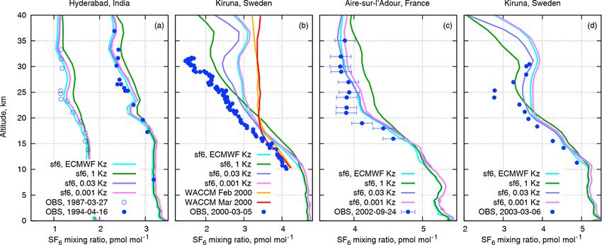
5846                                                                                     R. Kouznetsov et al.: Modelling age of air

Figure 5. Observed SF6 balloon profiles and corresponding daily-mean SILAM profiles for the date of observations. The observational
data obtained from Patra et al. (1997), Ray et al. (2014, 2017), and Engel et al. (2006) are for (a)–(d) correspondingly. The observation
uncertainties are about 2 % (1σ ) for Hyderabad profiles (a) and smaller than the size of the symbol for Kiruna profiles (b, d). The model
profiles from the WACCM model are from Ray et al. (2017).

cases. The most diffusive profile, 1-Kz, has the strongest de-            In all above cases, the 1-Kz profile is clearly far too dif-
pletion in the upper part but the largest deviation from the           fusive in the non-polar cases, whereas for the Kiruna cases
observations below 20 km. The intermediate-diffusion pro-              it overstates the lower part of the profiles and smears out the
file (0.03-Kz) is almost as close to the observations as the           vertical structure of the profiles further above the tropopause.
non-diffusive profile. Moreover, the 0.03-Kz profile has a             The SF6 profiles simulated with ECMWF-Kz and 0.001-Kz
minimum at the same altitude as the observed one, albeit the           match each other in all simulations, since vertical mixing is
modelled minimum is substantially less deep.                           negligible in both cases. The SF6 resulting from the 0.03-
   For comparison, Fig. 5b also contains monthly-mean pro-             Kz case appears to be the most realistic out of the four con-
files from the WACCM simulations by Ray et al. (2017).                 sidered simulations: they are close to the observed ones and
The WACCM profiles match very well with the observa-                   have the local minima at the correct altitudes for both Kiruna
tions below 17 km but turn nearly constant above, thus                 profiles.
under-representing the depletion of SF6 inside the polar
vortex. Monthly-mean SILAM profiles (not shown) were                   4.3   Evaluation of SF6 against MIPAS data
much closer to the plotted daily profiles than to the ones of
WACCM. However, the WACCM simulations did not include                  The MIPAS observations provide the richest observational
the electron attachment mechanism.                                     dataset for the stratospheric SF6 profiles. However, each in-
   For the mid-latitude profile in Fig. 5c from Aire-sur-              dividual observation has a substantial retrieval noise error,
l’Adour, France (43.7◦ N, 0.3◦ W), all SILAM profiles ex-              which is noticeably larger than the difference between the
cept for 1-Kz fall within the observational error bars pro-            observation and any of the SILAM simulations. The largest
vided together with the data by Ray et al. (2017). Similar to          diversity of the modelled SF6 profiles was observed in polar
the Kiruna case in Fig. 5b, the SILAM profiles are smoother            regions; therefore, below we show the mean profiles for each
than the observed ones and are unable to reproduce the sharp           season in the southern and the northern polar areas. Besides
transition at 20 km.                                                   that, we consider statistics of the model performance against
   Another profile from within the polar vortex (Fig. 5d) was          MIPAS measurements in the lower and upper stratosphere
observed at the same Kiruna site as the one in Fig. 5b, but            separately. For simplicity, we do not show the statistics for
three years later. The observed profile also has a minimum             the ECMWF-Kz runs, since they are very similar to the ones
that is much deeper than in the modelled profiles. Similar to          for 0.001-Kz.
the case in Fig. 5b, the 0.03-Kz profile is the only one that has         For the comparison, the daily-mean model profiles were
a pronounced minimum at the same altitude as the observed              co-located to the observed ones in space and time, after
one. The minimum is a result of the spring breakdown of the            which an averaging kernel of the corresponding MIPAS pro-
polar vortex when a regular downdraught ceases and atmo-               file was applied to the SILAM profile. For the comparison,
spheric layers decouple from each other. The reduced depth             we took only the data points with all of the following criteria
of the modelled minimum is probably caused by insufficient             met:
decoupling of the layers in the driving meteorology.
                                                                          – MIPAS visibility flag equals 1;

Atmos. Chem. Phys., 20, 5837–5859, 2020                                                   https://doi.org/10.5194/acp-20-5837-2020
R. Kouznetsov et al.: Modelling age of air 5847
The mean seasonal profiles of the SF6 mixing ratio for
southern and northern polar regions derived from the MIPAS
observations and the SILAM simulations for 2007 are given
in Fig. 6. In order to facilitate the comparison of our evalu-
ation with the earlier study of Kovács et al. (2017), we have
chosen the same year and same layout of the panels as Fig. 3
there. The main differences between Kovács et al. (2017) and
the current evaluation are the following.
– We used averages of co-located model profiles (bold
lines). The non-co-located seasonal- and area-mean
model profiles are given as thin dashed lines for com-
parison.
– We use a newer version of the MIPAS SF6 data with
considerably larger values (up to 0.6 pmol mol−1 ) in the
upper stratosphere, compared to the version that was
used by Kovács et al. (2017).
– The horizontal error bars for the observed data indicate
that the systematic error component is fully correlated
among the profiles and does not cancel out by averag-
ing or, in other words, the estimate of a possible bias,
as analysed by Stiller et al. (2008). These errors are of
the order of 4 % (below 30 km) up to 10 % (at 60 km).
The contribution of the retrieval noise error is essen-
tially negligible due to averaging. The error bars shown
by Kovács et al. (2017) are noticeably larger, probably
indicating that they are for the individual observed val-
ues rather than the uncertainties of the mean.
– We use 3 km vertical bins for the profiles to make the
points in the MIPAS profiles distinguishable.
– We also plot the vertical extent of the averaging kernels
corresponding to their half widths.
First of all, there is a substantial difference between the
co-located and non-co-located model profiles. The difference
Figure 6. Seasonal mean co-located SILAM SF6 and MIPAS pro- is caused by the uneven sampling of the atmosphere by the
files for 2007, for southern and northern polar regions. Typical satellite both in space and in time. In particular, MIPAS,
ranges covering 75 % of the averaging kernel are given with the being a polar-orbiting instrument, makes more profiles per
error bars at the right-hand side of each panel. The horizontal error unit area closer to the pole than further away. The differ-
bars indicate systematic uncertainties of the observations that are ence gets somewhat reduced if one uses equal weights for
fully correlated among profiles and do not cancel out when averag- all model grid cells instead of area-weighted averaging, es-
ing over a large number of measurements. Dashed lines are zonal-
pecially for wide latitude belts. The major difference comes
mean SILAM profiles for a given season taken without co-location.
probably from the inability of MIPAS to retrieve SF6 pro-
files in the presence of polar stratospheric clouds that clutter
– MIPAS averaging kernel diagonal elements exceed lower layers of the stratosphere and make the sampling of po-
0.03; lar regions quite uneven both in time and in the vertical. This
hypothesis agrees with the fact that the difference is most
– MIPAS retrieval vertical resolution, i.e. the full width at pronounced for the winter pole, especially for the South Pole
the half maximum of the row of the averaging kernel, is in JJA, and almost invisible at a summer pole.
better than 20 km; The comparison in Fig. 6 shows that the profiles from the
SILAM simulations agree quite well to the observations in
– MIPAS volume mixing ratio noise error of SF6 is less the altitude range below 20–25 km, with the most diffusive,
than 3 pmol mol−1 . 1-Kz, slightly overestimating the SF6 mixing ratios. In the
https://doi.org/10.5194/acp-20-5837-2020 Atmos. Chem. Phys., 20, 5837–5859, 20205848 R. Kouznetsov et al.: Modelling age of air
range above 25 km, the 1-Kz profiles indicate a decrease of Table 1. SF6 destruction rate after stopping the emissions and cor-
SF6 with altitude that is too fast. The 0.03-Kz profiles give responding lifetimes. Mid-2011 burden of 1.27 × 10⁹ moles is used
the best results up to ∼ 40 km, except for the South Pole in as a reference for the lifetime estimate.
JJA and the North Pole in DJF.
An interesting feature of the winter-pole MIPAS profiles Tracer, loss rate, lifetime,
is an increase of the SF6 mixing ratio above 40 km. This in- Kz scheme 103 mol yr−1 years
crease might be caused by issues with retrievals as the sys- passive, any Kz 0 ∞
tematic errors of the retrievals increase with altitude. How- SF6 , ECMWF-Kz 440 2900
ever, non-monotonic profiles can occur due to the mean at- SF6 , 0.001-Kz 480 2600
mospheric dynamics (see the non-co-located 0.001-Kz pro- SF6 , 0.01-Kz 760 1700
file in Fig. 6g). SF6 , 0.03-Kz 800 1540
None of the model setups are capable of reproducing SF6 , 0.1-Kz 960 1300
SF6 , 1-Kz 2160 590
the observations above 40 km. Wintertime poles also pose
a problem to the model. The disagreement indicates a defi-
ciency in the model representation of air flows in the upper
part of the domain caused by insufficient vertical resolution observation period; the same case indicates the least absolute
of ERA-Interim in the upper stratosphere and lower meso- bias.
sphere and a lack of pole-to-pole circulation. This discrep- In the range of 30–60 km altitudes (Fig. 8), the level of the
ancy is in line with the comparisons in Fig. 5 for polar re- retrieval noise is noticeably higher than in the lower strato-
gions. The model tends to overstate the SF6 content in the sphere. The least biased case is 1-Kz, which, however, has the
lower part of the polar vortex and understate it above 40 km. largest SD. The SDs of 0.03-Kz and 0.001-Kz are on par, but
We also computed statistical scores of the simulated SF6 the latter has the strongest bias. Thus for this altitude range
mixing ratios for each month of the MIPAS mission. The the intermediate-diffusivity case also shows the best perfor-
statistics were computed separately for the altitude ranges of mance.
10–35 km (Fig. 7) and 30–60 km (Fig. 8). As the difference Note the slight increase of the model bias after 2009,
in the statistical scores between the three selected simulations which is likely caused by our overestimating of the emission
is quite minor, we used only observations with the retrieval rates since that time (see Sect. 3.4). This increase of the bias
target noise error below 1 pmol mol−1 . does not appear in Fig. 8 due to the delay in the response
The root-mean-square error turned out to be mostly con- of the content in the upper layers to the changes in surface
trolled by the bias, and it does not allow for a clear distinc- emissions.
tion between the simulated cases. In order to disentangle the
effect of bias, we have calculated the standard deviation of 4.4 Lifetime of SF6 in the atmosphere
the model–measurement difference (SD), absolute bias, and
normalized mean bias (NMB): In order to estimate the atmospheric lifetime of SF6 , we
turned off the emission of all SF6 tracers in July 2016 and
D E1/2 let the model run until the end of 2018 without emissions
SD(pmol mol−1 ) = (M − hMi − O + hOi)2 , (15) (Fig. 9). The decrease of the simulated burden after the emis-
Bias(pmol mol−1 ) = hM − Oi , (16) sion stop can be used to estimate the removal rate from the
atmosphere.
M −O Time series of the total burden of SF6 in the atmosphere
NMB(%) = 2 · 100 %, (17)
M +O in the simulations are given in Fig. 9. For easier compari-
son to the observed mixing ratios, the burden has been nor-
where M and O are modelled and observed values, respec- malized with 1.78 × 10²⁰ moles – the total amount of air in
tively, and h·i denotes averaging over the selected model– the atmosphere – to get the mean mixing ratio. The tabu-
observation pairs for the given range of times and altitudes. lated values for the atmospheric burden of SF6 from Levin
Along with the SD, we have plotted the RMSE of the obser- et al. (2010) and Rigby et al. (2010) are given for compari-
vations due to the retrieval noise in the original MIPAS data, son. Since the removal of SF6 from the atmosphere is mostly
labelled as “MIPAS noise” in the top panels of Figs. 7 and 8. controlled by the transport towards the depletion layer, the
In the altitude range of 10–35 km, the SD of model– vertical exchange is the key controlling factor.
measurement difference is uniform in time with minor peaks The decrease of the atmospheric SF6 content after the
in August–September (Fig. 7). The level of the noise error emission stop is given in the inset in Fig. 9. As expected, after
constitutes about 85 % of the total model–measurement dif- July 2016 the content of passive SF6 stays constant, while the
ference. Application of the averaging kernel to the model others begin to decrease at a rate that depends on the trans-
profiles reduces the SD. The intermediate-diffusivity case, port properties in the stratosphere with the faster removal for
0.03-Kz, clearly shows the least SD uniformly over the whole the stronger eddy diffusivity. The removal rate is driven by
Atmos. Chem. Phys., 20, 5837–5859, 2020 https://doi.org/10.5194/acp-20-5837-2020You can also read