A mosaic of phytoplankton responses across Patagonia, the southeast Pacific and the southwest Atlantic to ash deposition and trace metal release ...
←
→
Page content transcription
If your browser does not render page correctly, please read the page content below
Ocean Sci., 17, 561–578, 2021
https://doi.org/10.5194/os-17-561-2021
© Author(s) 2021. This work is distributed under
the Creative Commons Attribution 4.0 License.

A mosaic of phytoplankton responses across Patagonia, the
southeast Pacific and the southwest Atlantic to ash deposition and
trace metal release from the Calbuco volcanic eruption in 2015
Maximiliano J. Vergara-Jara1,2 , Mark J. Hopwood3 , Thomas J. Browning3 , Insa Rapp4 , Rodrigo Torres2,5 ,
Brian Reid5 , Eric P. Achterberg3 , and José Luis Iriarte2,6
1 Programa  de Doctorado en Ciencias de la Acuicultura, Universidad Austral de Chile, Puerto Montt, Chile
2 Instituto
          de Acuicultura and Centro de Investigación Dinámica de Ecosistemas Marinos de Altas Latitudes (IDEAL),
Universidad Austral de Chile, Puerto Montt, Chile
3 GEOMAR, Helmholtz Centre for Ocean Research Kiel, 24148 Kiel, Germany
4 Department of Biology, Dalhousie University, Halifax, Nova Scotia, Canada
5 Centro de Investigación en Ecosistemas de la Patagonia (CIEP), Coyhaique, Chile
6 COPAS-Sur Austral, Centro de Investigación Oceanográfica en el Pacífico Sur-Oriental (COPAS),

Universidad de Concepción, Concepción, Chile

Correspondence: Mark J. Hopwood (mhopwood@geomar.de)

Received: 24 June 2020 – Discussion started: 3 July 2020
Revised: 16 February 2021 – Accepted: 16 February 2021 – Published: 21 April 2021

Abstract. Following the eruption of the Calbuco volcano in         caví diatom bloom can, however, only be speculated on due
April 2015, an extensive ash plume spread across northern          to the lack of data immediately preceding and following the
Patagonia and into the southeast Pacific and southwest At-         eruption. In the offshore southeast Pacific, a short-duration
lantic oceans. Here, we report on field surveys conducted          phytoplankton bloom corresponded closely in space and time
in the coastal region receiving the highest ash load fol-          to the maximum observed ash plume, potentially in response
lowing the eruption (Reloncaví Fjord). The fortuitous loca-        to Fe fertilisation of a region where phytoplankton growth is
tion of a long-term monitoring station in Reloncaví Fjord          typically Fe limited at this time of year. Conversely, no clear
provided data to evaluate inshore phytoplankton bloom dy-          fertilisation on the same timescale was found in the area sub-
namics and carbonate chemistry during April–May 2015.              ject to an ash plume over the southwest Atlantic where the
Satellite-derived chlorophyll a measurements over the ocean        availability of fixed nitrogen is thought to limit phytoplank-
regions affected by the ash plume in May 2015 were ob-             ton growth. This was consistent with no significant release of
tained to determine the spatial–temporal gradients in the off-     fixed nitrogen (NOx or NH4 ) from Calbuco ash.
shore phytoplankton response to ash. Additionally, leaching           In addition to the release of nanomolar concentrations of
experiments were performed to quantify the release from            dissolved Fe from ash suspended in seawater, it was ob-
ash into solution of total alkalinity, trace elements (dissolved   served that low loadings (< 5 mg L−1 ) of ash were an un-
Fe, Mn, Pb, Co, Cu, Ni and Cd) and major ions (F− , Cl− ,          usually prolific source of Fe(II) into chilled seawater (up to
SO2−       −    +      +      +    +
    4 , NO3 , Li , Na , NH4 , K , Mg
                                           2+ and Ca2+ ). Within   1.0 µmol Fe g−1 ), producing a pulse of Fe(II) typically re-
Reloncaví Fjord, integrated peak diatom abundances during          leased mainly during the first minute after addition to seawa-
the May 2015 austral bloom were approximately 2–4 times            ter. This release would not be detected (as Fe(II) or dissolved
higher than usual (up to 1.4 × 10¹¹ cells m−2 , integrated to      Fe) following standard leaching protocols at room temper-
15 m depth), with the bloom intensity perhaps moderated due        ature. A pulse of Fe(II) release upon addition of Calbuco
to high ash loadings in the 2 weeks following the eruption.        ash to seawater made it an unusually efficient dissolved Fe
Any mechanistic link between ash deposition and the Relon-         source. The fraction of dissolved Fe released as Fe(II) from

Published by Copernicus Publications on behalf of the European Geosciences Union.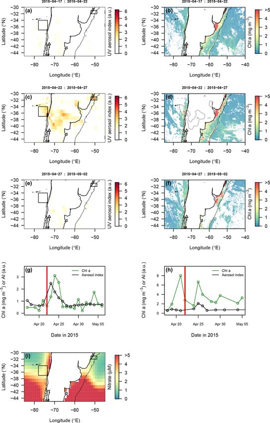
562                                      M. J. Vergara-Jara et al.: A mosaic of phytoplankton responses across Patagonia

Calbuco ash (∼ 18 %–38 %) was roughly comparable to lit-          tion (northern Patagonia, Chile) was predominantly de-
erature values for Fe released into seawater from aerosols        posited over an inshore and coastal region (Romero et al.,
collected over the Pacific Ocean following long-range atmo-       2016) (Fig. 1). This led to visible high ash loadings in af-
spheric transport.                                                fected surface waters in the weeks after the eruption (Fig. 2),
                                                                  providing a case study for a concentrated ash deposition
                                                                  event in a coastal system: Reloncaví Fjord, which is the
                                                                  northernmost fjord of Patagonia. It receives the direct dis-
1   Introduction                                                  charge from three major rivers, creating a highly stratified
                                                                  and productive fjord system in terms of both phytoplankton
Volcanic ash has long been considered a large, intermit-          biomass and aquaculture production of mussels (González et
tent source of trace metals to the ocean (Frogner et al.,         al., 2010; Molinet et al., 2017; Yevenes et al., 2019). Here,
2001; Sarmiento, 1993; Watson, 1997), and its deposition is       we combine in situ observations from moored arrays, which
now deemed a sporadic generally low-macronutrient, high-          were fortuitously deployed in Reloncaví Fjord (Vergara-Jara
micronutrient supply mechanism (Ayris and Delmelle, 2012;         et al., 2019), with satellite-derived chlorophyll data for off-
Jones and Gislason, 2008; Lin et al., 2011). As volcanic          shore regions subject to ash deposition and leaching exper-
ash can be a regionally significant source of allochthonous       iments carried out on ash collected from the fjord region in
inorganic material to affected water bodies, volcanic erup-       order to investigate the inorganic consequences of ash ad-
tions have the potential to dramatically change light avail-      dition to natural waters. We thereby evaluate the potential
ability, the carbonate system, properties of sinking particles    positive and negative effects of ash from the 2015 Calbuco
and ecosystem dynamics (Hoffmann et al., 2012; Newcomb            eruption on marine phytoplankton in three geographical re-
and Flagg, 1983; Stewart et al., 2006). Surveys directly un-      gions: Reloncaví Fjord and the areas of the southeast Pacific
derneath the ash plume from the 2010 eruption of Eyjaf-           and southwest Atlantic oceans beneath the most intense ash
jallajökull (Iceland) over the North Atlantic found, among        plume.
other biogeochemical perturbations, high dissolved Fe (dFe)
concentrations of up to 10 nM in affected surface seawater
(Achterberg et al., 2013) which could potentially result in       2     Materials and methods
enhanced primary production. The greatest potential positive
effect of ash deposition on marine productivity would gen-        2.1    Study area
erally be expected in high-nitrate, low-chlorophyll (HNLC)
areas of the ocean (Hamme et al., 2010; Mélançon et al.,          The Calbuco volcano (Fig. 1) is located in a region with large
2014), where low Fe concentrations are a major factor lim-        freshwater reservoirs and in close proximity to Reloncaví
iting primary production (Martin et al., 1990; Moore et al.,      Fjord. The predominant bedrock type is andesite (López-
2013). Therefore, special interest is placed on the ability of    Escobar et al., 1995). Reloncaví Fjord is 55 km long and re-
volcanic ash to release dFe, and other bio-essential trace met-   ceives freshwater from three main rivers, the Puelo, Petro-
als such as Mn (Achterberg et al., 2013; Browning et al.,         hué, and Cochamó, with mean stream flows of 650, 350
2014; Hoffmann et al., 2012), into seawater. In contrast, apart   and 100 m3 s−1 respectively (León-Muñoz et al., 2013).
from inducing light limitation, there are several adverse ef-     River discharge strongly influences seasonal patterns of pri-
fects of ash deposition on aquatic organisms; these include       mary production across the region, supplying silicic acid
metal toxicity (Ermolin et al., 2018), particularly under high    and strongly stratifying the water column (Castillo et al.,
dust loading (Hoffmann et al., 2012), and the ingestion of        2016; González et al., 2010; Torres et al., 2014). Seasonal
ash particles by filter-feeders, phagotrophic organisms or fish   changes in light availability rather than macronutrient sup-
(Newcomb and Flagg, 1983; Wolinski et al., 2013). Transient       ply are thought to control marine primary production across
shifts to low pH have also been reported in some (but not         the Reloncaví region, with high marine primary production
all) ash leaching experiments and in some freshwater bod-         (> 1 g C m−2 d−1 ) throughout austral spring, summer and
ies following intense ash deposition events, suggesting that      early autumn (González et al., 2010).
significant ash deposition on weakly buffered aquatic envi-          On 22 April 2015 the Calbuco volcano erupted after
ronments can also impact and perturb their carbonate system       54 years of dormancy. Two major eruption pulses lasted < 2 h
(Duggen et al., 2010; Jones and Gislason, 2008; Newcomb           on 22 April and 6 h on 23 April, releasing a total volume
and Flagg, 1983). Therefore, the greatest negative impact of      of 0.27 km3 of ash which was projected up to 20 km a.s.l.
ash on primary producers would be expected closest to the         (above sea level) (Van Eaton et al., 2016; Romero et al.,
source, where the ash loading is highest, and in areas where      2016). Ash layers that were several centimetres thick were
macronutrients or light, rather than trace elements, limit pri-   deposited mainly to the northeast of the volcano in subse-
mary production.                                                  quent days (Romero et al., 2016). A smaller eruption oc-
   In contrast to the 2010 Eyjafjallajökull plume over the        curred on 30 April projecting ash 4–5 km a.s.l. which was
North Atlantic, the 2015 ash plume from the Calbuco erup-         then mainly deposited south of the volcano. Smaller vol-

Ocean Sci., 17, 561–578, 2021                                                         https://doi.org/10.5194/os-17-561-2021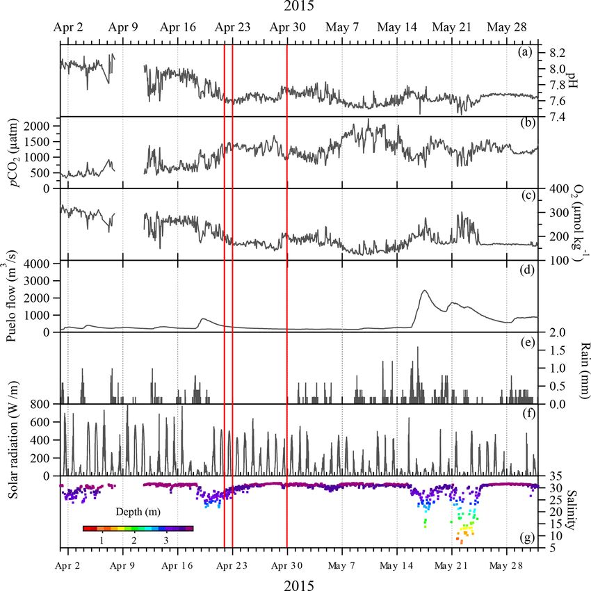
M. J. Vergara-Jara et al.: A mosaic of phytoplankton responses across Patagonia 563
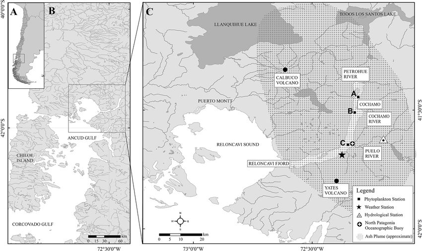
Figure 1. The Calbuco region showing the location of Reloncaví Fjord, three major rivers (the Petrohué, Cochamó and Puelo) discharging
into the fjord, the three stations (black squares; panel c) used to assess changes in phytoplankton abundance following the eruption, a
hydrological station that monitors the Puelo River flow, a weather station and the location of a long-term mooring within the fjord. The
approximate extent of the ash plume in the week following the first eruption is illustrated, as estimated in technical reports issued by the
Servicio Nacional de Geología y Minería (Chile).
umes of ash were released semi-continuously for 3 weeks 2.2 Ash samples – trace metal leaching experiments
after the main eruption, leading to intermittent ash deposi-
tion events. Fortuitously, as part of a long-term deployment,
On 6 May (2015, Cochamó, Chile, approximately 30 km
an ocean acidification buoy in the middle of Reloncaví Fjord
from the volcano) after the third (and smallest) eruptive pulse
(Vergara-Jara et al., 2019) and an associated meteorological
of ash from the Calbuco volcano (Fig. 2a) and with the
station close to the volcano (Fig. 1) were well placed to as-
volcano still emitting material, ash was collected using a
sess the impact of ash deposition immediately after the erup-
plastic tray wrapped with plastic sheeting (40 cm × 94 cm).
tion. To complement data from these facilities, after the re-
The plasticware was left outside for 24 h until sufficient ash
gional evacuation order was removed, weekly sampling cam-
(∼ 500 g) was collected to provide a bulk sample. Ambient
paigns were conducted in the fjord commencing 1 week after
weather over the period of ash collection (and the preceding
the eruption. The National Geology and Mining Service (Ser-
day) was dry (no precipitation). The collected ash was dou-
vicio Nacional de Geología y Minería, SERNAGEOMIN)
ble sealed in low-density polyethylene (LDPE) plastic bags
produced daily technical reports including the estimated
and stored in the dark. A subsample was analysed for particle
area of ash dispersion (http://sitiohistorico.sernageomin.cl/
size using a Mastersizer 2000 at the University of Chile.
volcan.php?pagina=4&iId=3, last access: 1 February 2021).
Ash may affect in situ phytoplankton dynamics in several
This information was used to create a reference aerial extent
ways – for example, by moderating the carbonate system,
of ash deposition for the week after the eruption (Fig. 1c).
macronutrient availability and/or micronutrient availability.
This approximation represents a full week of coverage for
As micronutrient (e.g. Fe and Mn) availability is expected to
this dynamic feature.
be the main chemical mechanism via which phytoplankton
dynamics in the offshore marine environment could be af-
fected, we primarily focus our investigation on the release of
dissolved trace metals from ash in seawater. However, to rule
https://doi.org/10.5194/os-17-561-2021 Ocean Sci., 17, 561–578, 2021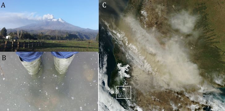
564                                       M. J. Vergara-Jara et al.: A mosaic of phytoplankton responses across Patagonia

out other potential effects, we also conduct complementary         changes on timescales of hours to days (Duggen et al., 2007;
leaches to assess the significance of changes to total alkalin-    Frogner et al., 2001; Jones and Gislason, 2008).
ity and macronutrient availability (Table 1). For trace metal          A variety of leaches were conducted in deionised water,
leaches, a variety of methods have been used in the litera-        brackish (fjord) water or offshore South Atlantic seawater
ture (Duggen et al., 2010; Witham et al., 2005) depending          (Table 1) with the choice of leaching conditions based on
on the purpose of specific studies. Deionised water leaches        the expected environmental significance in different water
with ash loadings that are high in an offshore environmental       masses. Offshore oligotrophic seawater for incubation exper-
context are preferable for intercomparison studies. The trace      iments was collected from an underway transect of the mid-
metals released under such conditions are, however, difficult      South Atlantic (across 40◦ S) using a towfish and trace metal
to compare quantitatively to metal exchange processes in the       clean tubing in a 1 m3 high-density polyethylene tank which
ambient marine environment, especially for elements such           had been pre-rinsed with 1 M HCl. This water was stored
as Fe where solubility is strongly influenced by pH, salin-        in the dark for > 12 months prior to use in leaching exper-
ity and the nature of dissolved organic carbon present (Baker      iments and was filtered (AcroPak1000 capsule 0.8/0.2 µm
and Croot, 2010). For prior work conducted specifically us-        filters) when subsampling a batch for use in all leaching
ing volcanic ash in seawater, three main methods have been         experiments. All labware for trace metal leaching experi-
employed: suspension experiments followed by analysis of           ments was pre-cleaned with Mucasol and 1 M HCl. The
the leachate, flow-through reactors and continuous voltam-         125 mL LDPE bottles (Nalgene) for trace metal leach ex-
metric determination of dFe concentrations in situ during          periments were pre-cleaned using a three-stage procedure
suspension experiments (Table S1 in the Supplement). The           with three deionised water (Milli-Q, Millipore, conductiv-
most commonly used ash : solute ratio in prior seawater ex-        ity 18.2 M cm−1 ) rinses after each stage (3 d in Mucasol,
periments is 1 : 400 (g : mL), with leach lengths varying from     1 week in 1 M HCl, 1 week in 1 M HNO3 ).
15 min to 24 h (Table S1). Conversely, incubation experi-              Leach experiments were conducted by adding a pre-
ments designed to test the response of marine phytoplankton        weighed mass of ash into 100 mL South Atlantic seawater,
to ash deposition have used lower ash : solute ratios of 1 : 400   gently mixing the suspension for 10 min, and then syringe fil-
to 1 : 107 which are based on estimates of the ash loading ex-     tering the suspension (0.2 µm, polyvinylidene fluoride, Mil-
pected to be mixed within the offshore surface mixed layer         lipore). Eight different ash loadings from 2 to 50 mg L−1
underneath ash plumes (Browning et al., 2014; Hoffmann et          were used, which were selected to be environmentally rel-
al., 2012). Existing data suggest that the ash : solute ratio is   evant and comparable to prior incubation experiments, with
not a major factor in determining the release behaviour of         each treatment run in triplicate. Samples for dissolved trace
Fe from ash; nevertheless, this is acknowledged to be diffi-       metals (Fe, Cd, Pb, Ni, Cu, Co and Mn) were acidified within
cult to assess due to other differences between experimental       1 d of collection by the addition of 140 µL concentrated HCl
set-ups used to date (Duggen et al., 2010). Both the age of        (UpA grade, ROMIL) and analysed by inductively coupled
particles since collection and the organic carbon content of       plasma mass spectroscopy following pre-concentration ex-
seawater are, however, known to be critical factors influenc-      actly as per Rapp et al. (2017).
ing the exchange of Fe (and other trace elements) following            Leach experiments specifically to measure Fe(II) release
any aerosol deposition into seawater (Baker and Croot, 2010;       were conducted in a similar manner but in cold seawater
Duggen et al., 2010). Whilst the UV treatment of seawater          with continuous in-line analysis (5–7 ◦ C; see Table S2 in
has been used in some experiments (to remove a large part          the Supplement) due to the rapid oxidation rate of Fe(II) at
of any natural organic ligands present, Duggen et al., 2007;       room temperature (∼ 21 ◦ C), which makes the accurate mea-
Jones and Gislason, 2008), and a strong synthetic organic lig-     surement of Fe(II) concentrations challenging (Millero et al.,
and has been added in others (to impede dissolved Fe precip-       1987). For these experiments, a pre-weighed mass of ash was
itation; Duggen et al., 2007; Olgun et al., 2011; Simonella        added to 250 mL of South Atlantic seawater and manually
et al., 2015), to improve reproducibility and standardisation,     shaken for approximately 1 min, using an expanded loading
these steps are not well suited specifically for investigating     range from 0.2 to 4000 mg L−1 . Fe(II) was measured via flow
the release of Fe(II) from ash. Thus, in this study, we adopt      injection analysis using luminol chemiluminescence (Jones
ash : solute ratios comparable to the lower end of the range       et al., 2013) without pre-concentration or filtration. The in-
used in leaching experiments and comparable to the range           flow line feeding the flow injection apparatus was positioned
used in incubation experiments. Seawater was used after pro-       inside the ash suspension immediately after mixing and mea-
longed storage in the dark (to reduce biological activity to       surements begun thereafter at a 2 min resolution. Reported
low background levels) and without UV treatment (to main-          mean values (± standard deviation) are determined from the
tain an environmentally relevant level of natural organic ma-      Fe(II) concentrations measured 2–30 min after adding ash
terial in solution). A short leaching time (10 min + filtration)   into solution. Calibrations were run daily using standard ad-
was adopted to minimise bottle effects and recognising that        ditions of 0.2–10 nM Fe(II) to aged South Atlantic seawa-
most prior work suggests a large fraction of Fe release oc-        ter at the same temperature with integrated peak area used
curs on short timescales (minutes), followed by more gradual       to construct calibration curves. Following each leaching ex-

Ocean Sci., 17, 561–578, 2021                                                          https://doi.org/10.5194/os-17-561-2021
M. J. Vergara-Jara et al.: A mosaic of phytoplankton responses across Patagonia                                              565

periment, the apparatus was rinsed with 0.1 M HCl (reagent       leaching experiment, AT was analysed by titration of unfil-
grade) followed by flushing with deionised water to ensure       tered 5 mL subsamples to a pH 4.5 end point (bromocre-
the removal of ash particles. Blank measurements before and      sol green–methyl red) using a Dosimat (Metrohm Inc) and
after Fe(II) measurements from experiments with different        0.02 N H2 SO4 titrant. Alkalinity was calculated as CaCO3
ash loadings verified that there was no discernable interfer-    equivalents following APHA (American Public Health As-
ence from ash particles in the Fe(II) flow-through measure-      sociation) 2005 Method 2320 (2320 alkalinity and titration
ments. Fe(II) leaches were conducted 2 weeks, 4 months and       method). Additional 5 mL subsamples were filtered, stored
9 months after the eruption. Fe(II) leaches 2 weeks after the    at 4 ◦ C and analysed within 3 d for major ions (F− , Cl− ,
eruption were run for 30 min. Fe(II) leaches 4 or 9 months       SO2−        −     +    +      +    +
                                                                     4 , NO3 , Li , Na , NH4 , K , Mg
                                                                                                           2+ and Ca2+ ) using

after the eruption were run for 1 h to further investigate the   a Dionex™ 5000 ion chromatography system with eluent
temporal development of the Fe(II) concentration. The trace      generation (APHA). All measurements were then corrected
metal leach experiments (above) were conducted at the same       for initial water concentrations prior to ash addition. Satura-
time as the first Fe(II) incubation experiments (2 weeks after   tion indices for species in solution following leaching from
ash collection).                                                 < 63 µm ash particles were obtained from the MINTEQ 3.1.
   For trace metal leaches, the initial (mean ± standard de-     IAP (ion activity product) chemical equilibrium model (see
viation) dissolved trace metal concentrations were deducted      Table S6 in the Supplement).
from the final concentrations, in order to calculate the net
change as a result of ash addition. For Fe(II) measurements,     2.4   Environmental data – continuous Reloncaví Fjord
background levels of Fe(II) were below detection (< 0.1 nM)            monitoring
and so no deduction was made.
                                                                 High-temporal-resolution (hourly) in situ measurements
2.3   Ash samples – deionised and brackish water                 were taken in the Reloncaví Fjord (Fig. 1c, North Patago-
      leaching experiments                                       nia Oceanographic Buoy) at 3 m depth using submersible au-
                                                                 tonomous moored instrument (SAMI) sensors that measured
Fresh brackish subsurface water from the Patagonia study re-     spectrophotometric CO2 and pH (DeGrandpre et al., 1995;
gion was obtained from the Aysén Fjord, at Ensenada Baja         Seidel et al., 2008) (Sunburst Sensors, LLC) and an SBE
(45◦ 210 S, 72◦ 400 W; salinity 16.3), close to the Coyhaique    37 MicroCAT CTD-ODO (Sea-Bird Electronics) that mea-
laboratory (Aysén region, Chile) and free from the influ-        sured temperature, conductivity, depth and dissolved O2 , as
ence of ash from the 2015 eruption. The oceanographic con-       per Vergara-Jara et al. (2019). Sensor maintenance and qual-
ditions in these waters are similar to the adjacent Relon-       ity control is described by Vergara-Jara et al. (2019). The er-
caví Fjord (Cáceres et al., 2002). Deionised water, along        ror in pCO2 concentrations is estimated to be 5 % at most
with the Aysén Fjord brackish water, were used for leach-        and arises mainly due to a non-linear sensor response and
ing experiments using two size fractions of ash, follow-         reduced sensitivity at high pCO2 levels > 1500 ppm (De-
ing the general recommendations of Duggen et al. (2010)          Grandpre et al., 1999). The SAMI pH instruments used an
and Witham et al. (2005), to consider the effects of differ-     accuracy test instead of a calibration procedure (Seidel et al.,
ent size fractions and leachates. Leaches were conducted in      2008). With the broad pH and salinity range found in the
50 mL LDPE bottles filled with either 40 mL of brackish or       fjord, pH values are subject to a maximum error of ± 0.02
deionised water with four replicates of each treatment. Bot-     (Mosley et al., 2004).
tles were incubated inside a mixer at room temperature af-          A meteorological station (HOBO U30, Fig. 1) measured
ter the addition of 0.18 g of ash, using two ash size frac-      air temperature, solar radiation, wind speed and direction,
tions (< 63 and 250–1000 µm) which were separated using          rainfall, and barometric pressure every 5 min. Puelo River
sieves (ASTM E11 specification, W. S. Tyler). The mass dis-      streamflow was obtained from the Carrera Basilio hydrolog-
tribution of the ash as determined by sieving was 4.54 %         ical station (Fig. 1), run by Dirección General de Aguas de
> 2360 µm, 6.85 % < 2360 and > 1000 µm, 31.12 % < 1000           Chile, via a data request (submitted via https://snia.mop.gob.
and > 250 µm, 24.14 % < 250 and > 125 µm, 18.04 % < 125          cl/BNAConsultas/reportes, last access: 22 February 2019).
and > 63 µm, and 15.31 % < 63 µm. Thus, the dominant size
fraction by mass was the 250–1000 µm fraction, which was         2.5   Field surveys in Reloncaví Fjord post-eruption
analysed in addition to the finest fraction (< 63 µm) with the
greatest surface area to mass ratio. The sampling times were     During May 2015, weekly field campaigns were undertaken
at time zero (defined as just after the addition of the ash      in the Reloncaví Fjord. Phytoplankton samples were col-
and a few minutes of mixing) and 2 and 24 h later. Leach-        lected at three depths (1, 5 and 10 m) for taxonomic char-
ing experiments conducted with brackish water were anal-         acterisation and abundance determination at three stations
ysed for total alkalinity (AT ) via a potentiometric titration   (Fig. 1c) using a 5 L GO-FLO bottle. Samples for cell counts
using reference standards (Haraldsson et al., 1997), ensuring    were stored in clear plastic bottles (300 mL) and preserved
a reproducibility of < 2 µmol kg−1 . For the deionised water     in a Lugol iodine solution. From each sample, a 10 mL sub-

https://doi.org/10.5194/os-17-561-2021                                                         Ocean Sci., 17, 561–578, 2021
566 M. J. Vergara-Jara et al.: A mosaic of phytoplankton responses across Patagonia
Table 1. Summary of different leaching experiments and samples.
Ash/particle source Deionised water Brackish (fjord) South Atlantic Number of replicates
leaches water seawater
Calbuco ash, sieved Total alkalinity, ion and Total alkalinity – 4
< 63 µm macronutrients
Calbuco ash, sieved Total alkalinity, ion and Total alkalinity – 4
250–1000 µm macronutrients
Calbuco ash, – – Trace metals, Fe(II) 3 for trace elements,
unsieved 1 time series for Fe(II)
sample was placed in a sedimentation chamber and left to downloaded for the same time period. Daily images were
settle for 16 h. The complete chamber bottom was scanned composited into 5 d mean averages.
at 200× to enumerate the organisms, and the result was ex-
pressed as number of phytoplankton cells per litre of seawa-
ter (Hasle, 1978). Phytoplankton were identified to genus or 3 Results
species level, when possible, and divided into diatoms and
3.1 In situ observations
dinoflagellates. Samples were analysed using an Olympus
CKX41 inverted phase contrast microscope and the Uter- The Calbuco ash plume reached up to a height of 20 km and
möhl method (Utermöhl, 1958). The phytoplankton commu- was dispersed hundreds of kilometres across Patagonia and
nity composition was then statistically analysed in R (R Core the Pacific and Atlantic oceans (Fig. 2) (Van Eaton et al.,
Team, 2020; R Studio V 1.2.5033) using general linear mod- 2016; Reckziegel et al., 2016; Romero et al., 2016). The ash
els in order to find statistically significant differences be- loading in water bodies near the cone was visually observed
tween dates and group abundances. Additionally, as part of to be high, especially near the Petrohué River catchment that
a long-term monitoring programme at station C (Fig. 1c), drains into the head of the Reloncaví Fjord. This ash load-
chlorophyll a samples were retained from six depths (1, 3, 5, ing in the fjord was clearly visible on 6 May 2015 when ash
7, 10 and 15 m) on six occasions during March–May 2015. samples were collected for leaching experiments (Fig. 2).
Chlorophyll a was determined by fluorometry after filtering Carbonate chemistry data from the Reloncaví Fjord moor-
250 mL of sampled water through GF/F filters (Whatman) as ing demonstrated that the pH declined and the pCO2 in-
per Welschmeyer (1994). Two additional profiles close to sta- creased in the week prior to the first eruption (22 April,
tion C were obtained from Yevenes et al. (2019). Integrated Fig. 3). Oxygen and pH reached a minimum and pCO2
chlorophyll a (mg m−2 ) and diatom abundance (cells m−2 ) reached a maximum during the time period from 7 to 14 May,
were determined to 15 m depth. Chlorophyll a within Relon- which indicates a state of high respiration. In this stratified
caví Fjord is invariably concentrated in the upper ∼ 10 m environment, the brackish fjord surface layer generally has
(González et al., 2010; Yevenes et al., 2019); thus, for com- low pH and high pCO2 , with seasonal changes in salinity
parison to prior reported data integrated to 10 m, only a small and respiration leading to a large annual range of pCO2 and
difference is anticipated. For all profiles considered herein, pH (Vergara-Jara et al., 2019). The depth of the sensors var-
there is a 20 % difference between integrating to 10 m or ied temporally due to changes in tides and river flow. This
15 m depth. accounts for some of the variation in measured salinity due
to the strong salinity gradient with depth in the brackish sur-
2.6 Satellite data face waters (Fig. 3). Therefore, any changes in pCO2 or
pH occurring as a direct result of the eruptions (or asso-
ciated ash deposition) are challenging to distinguish from
Daily, 4 km resolution chlorophyll a images from the
background variation due to short-term (intra-day) or sea-
MODIS Aqua sensor (Ocean Color Index, OCI, algorithm;
sonal shifts in the carbonate system which are pronounced
Hu et al., 2012) were downloaded from the NASA Ocean
in this dynamic and strongly freshwater-influenced environ-
Color website (https://oceancolor.gsfc.nasa.gov, last access:
ment (Fig. 3). Freshwater discharge from the Puelo increased
1 June 2020) for the period from 4 April to 2 May 2015. As
sharply from 16 May which is an annually recurring event
the UV aerosol index largely reflects strongly UV-absorbing
(González et al., 2010).
(dust) aerosols (Torres et al., 2007), this was used as a proxy
for the spatial extent and loading of the ash plume. The UV
aerosol index product from the Ozone Monitoring Instru-
ment (OMI) on the Earth Observing System (EOS) Aura was
Ocean Sci., 17, 561–578, 2021 https://doi.org/10.5194/os-17-561-2021M. J. Vergara-Jara et al.: A mosaic of phytoplankton responses across Patagonia 567
Figure 2. (a) Calbuco volcano ash plume 6 May 2015. (b) Reloncaví Fjord water with atypical high turbidity due to the ash loading, Cochamó
town 6 May. (c) Ash cloud visible on MODIS Aqua satellite from the NASA Earth Observatory, 23 April (http://earthobservatory.nasa.gov/
NaturalHazards/view.php?id=85767&eocn=home&eoci=nh, last access: 1 February 2021). The highlighted box in panel (c) corresponds to
Fig. 1c.
3.2 Phytoplankton in Reloncaví Fjord post-eruption 3.3 Total alkalinity and macronutrients in leach
experiments
Phytoplankton abundances observed in May 2015 within
Reloncaví Fjord were assessed by diatom cell counts and
Size analysis of the collected ash determined a mean particle
chlorophyll a concentrations (Table S3 in the Supplement)
diameter of 339 µm. Small ash particles (< 63 µm) resulted
and were proportionate to or higher than those previously ob-
in minor or no significant changes to AT in brackish fjord
served in the region (Fig. 4). When comparing observations
waters (Fig. 5). With larger ash particles (250–1000 µm), no
to prior data from González et al. (2010), it should be noted
effect was evident. Conversely, a leaching experiment with
that there is a slight depth discrepancy (earlier work was inte-
deionised water showed a small increase in AT (Fig. 5) for
grated to 10 m depth rather than the 15 m used herein). How-
both size fractions. By increasing the AT of freshwater, ash
ever, as the phytoplankton bloom is overwhelmingly present
would act to increase the buffering capacity of river out-
within the upper 10 m, these data do provide a useful com-
flow into a typically weak carbonate system like the Relon-
parison. Diatom abundance integrated to 15 m depth peaked
caví Fjord (Vergara-Jara et al., 2019). However, the absolute
at stations B and C around 14 May, with notably lower abun-
change in AT was relatively small despite the large ash load-
dances at the innermost station A (Fig. 4). The highest mea-
ing used in all incubations (< 20 µmol kg−1 AT for ash load-
sured chlorophyll a concentrations were on 30 April at sta-
ing > 4 g L−1 ); therefore, it is expected that the direct effect
tion C; chlorophyll a values then declined to much lower
of ash on AT in situ was limited. Other effects on carbonate
concentrations in late May, which is expected from patterns
chemistry may, however, arise due to ash moderating the tim-
in regional primary production (González et al., 2010). No
ing and intensity of primary production and, thus, biological
measurements were available for 10–30 April 2015 (Fig. 4);
pCO2 drawdown.
thus, it is not possible to determine the timing of the onset of
Ion chromatography results for Na+ , K+ , Ca2+ , F− , Cl− ,
the austral autumn phytoplankton bloom with respect to the 2−
NO− 3 and SO4 showed that ion inputs were generally higher
volcanic eruptions from the available chlorophyll a or diatom
in the presence of smaller ash size particles (Table 2), as has
data. However, within this time period, the mooring at station
been reported previously (Jones and Gislason, 2008; Óskars-
C (Fig. 3) did record a modest increase in pH and O2 from
son, 1980; Rubin et al., 1994). The leaching from ash com-
28 to 29 April, during a time period when river discharge and
ponents into deionised water occurred almost instantly with
salinity were stable, which could be indicative of the autumn
limited or no increases in leached concentrations observed
phytoplankton bloom onset.
between 0, 2 and 24 h (Table 2). For larger particles, there
was less release of most ions. In the case of Ca2+ and SO2− 4 ,
a more gradual leaching effect was apparent (Table 2). The
concentrations of NO− +
3 and NH4 were generally below de-
tection suggesting that ash was a minor source of fixed-
nitrogen into solution. These observations are consistent with
the trends in prior work using a range of volcanic ash and
https://doi.org/10.5194/os-17-561-2021 Ocean Sci., 17, 561–578, 2021568 M. J. Vergara-Jara et al.: A mosaic of phytoplankton responses across Patagonia
Figure 3. Continuous data from the Reloncaví Fjord mooring and nearby hydrological and weather stations for April–May 2015. The vertical
red lines mark the eruption dates. All locations are marked in Fig. 1. Carbonate chemistry and salinity data are from Vergara-Jara et al. (2019).
Wind and tidal mixing caused small changes in the depth of the sensors which are shown alongside the salinity data.
incubation conditions (Duggen et al., 2010; Witham et al., tration of metals in South Atlantic seawater should, however,
2005). Major ion analysis was only conducted in deionised also be considered when interpreting the trends. The magni-
water, as no significant changes would be observable for tude of changes in Cd and Ni concentrations were smallest
most of these ions in brackish or saline waters under the same relative to both the initial concentration and the standard de-
conditions. viation on the initial concentration (0.38 ± 0.04 nM Cd and
6.58 ± 0.76 nM Ni respectively). Thus, it would be difficult
3.4 Trace elements in leach experiments to extract a clear relationship irrespective of their chemical
behaviour. For other elements (Fe, Co and Pb), non-linearity
between ash addition and trace metal concentrations as well
The release of nanomolar concentrations of dissolved Fe and
as some negative changes in concentrations both likely re-
Mn was evident when ash was resuspended in aged seawa-
flect scavenging of metal ions onto ash particle surfaces (Ro-
ter for 10 min (Fig. 6). The net release of dissolved metals
gan et al., 2016). Fe, Co and Pb are all scavenged-type ele-
proceeded with varying relationships with ash loading over
ments, and so increasing the surface area of ash present may
the applied gradient (2–50 mg L−1 ). Dissolved Mn, Pb, Cu
affect the net change in metal concentration. The divergence
and Co release exhibited significant (pM. J. Vergara-Jara et al.: A mosaic of phytoplankton responses across Patagonia 569
Table 2. Major ion and macronutrient concentrations in micromoles per litre (µmol L−1 ) leached from the two size fractions of ash (< 63 and
250–1000 µm) into deionised water (b.d. stands for below detection). Shown are mean values, with the standard deviation in parentheses (n =
4). Also shown are mass normalised values (µmol g−1 ash) and a comparison to the range of values reported by Jones and Gislason (2008);
the latter is referred to as “Range (lit.)” in the table.
Time [h] Na+ K+ Ca2+ F− Cl− SO2−
4 NO−
3 NH+
4
Detection limit 0.17 0.43 0.30 0.28 1.31 1.64 0.34 0.13
Procedural blank b.d. b.d. 0.39 b.d. b.d. b.d. b.d. b.d.
250–1000 µm [µmol L−1 ] 0.1 3.4 (2.8) 0.83 (0.3) 18.3 (3.3) 0.16 (0.05) 3.7 (1.9) 3.7 (2.2) b.d. 0.15 (0.2)
2 5.1 (2.0) 1.0 (0.2) 18.5 (4.5) 0.21 (0.08) 4.4 (1.6) 4.9 (2.0) b.d. 0.38 (0.4)
24 7.3 (0.1) 1.4 (0.2) 23.4 (3.2) 0.52 (0.18) 5.7 (0.5) 8.3 (2.1) b.d. b.d.
< 63 µm [µmol L−1 ] 0.1 16.2 (12.7) 3.2 (0.3) 25.1 (5.4) 0.29 (0.0) 17.1 (13.6) 13.5 (1.3) 0.53 (0.2) 1.70 (1.1)
2 16.7 (1.0) 3.8 (0.1) 31.8 (2.7) 0.63 (0.2) 15.2 (0.9) 19.0 (0.3) b.d. 0.52 (1.0)
24 17.3 (0.8) 3.9 (0.3) 33.8 (3.3) 0.69 (0.3) 14.6 (1.0) 18.8 (0.5) b.d. 1.32 (2.6)
< 63 µm [µmol g−1 ash] 24 3.84 0.87 7.50 0.15 3.25 4.18 0.048 0.29
Range (lit.) 1.5–84.3 0.1–5.4 0.6–589 0.1–9 2–92.9 1–554 0–6.4 0.3–0.6
Figure 4. Changes in integrated (0–15 m) diatom abundance and
Figure 5. Total alkalinity released after leaching 4.5 g L−1 of ash of
chlorophyll a for Reloncaví Fjord in April–May 2015. Locations are
two size fractions (< 63 and 250–1000 µm) in deionised water (DI
as per Fig. 1; the eruption dates are marked with red lines. Historical
water) and brackish water. T0 is “time zero” and was measured after
diatom data from Reloncaví Sound (2001–2008, integrated to 10 m
1 min of mixing; T2H was measured after 2 h of mixing; T24H was
depth, mean ± standard error, González et al., 2010) and additional
measured after 24 h of mixing. n = 4 for all treatments (mean ±
chlorophyll data from 2015 (“Station 3” from Yevenes et al., 2019,
standard deviation plotted). The initial (pre-ash addition) alkalinity
approximately corresponding to station C herein) are also shown.
is marked by a black dot superimposed on the left T0 . Source data
are provided in the Supplement (Table S4).
availability, whereas the release of dissolved Fe is more de-
pendent on the nature of organic material present in solution. diate sea surface temperature for the high-latitude ocean. A
In addition to the release of dFe in solution, which gener- sharp decline in Fe(II) dissolution efficiency with increasing
ally exists as Fe(III) species in oxic seawater (Gledhill and ash load was also evident (Fig. 7). Both the highest Fe(II)
Buck, 2012), the release of Fe(II) was evident on a similar concentration and the highest net release of Fe(II) were ob-
timescale when cold (5–7 ◦ C) aged South Atlantic seawa- served at the lowest ash loading (Figs. 7 and S2). The Fe(II)
ter was used as leachate (Fig. 7). The half-life of Fe(II) de- concentration following dust addition into seawater was pos-
creases more than 10-fold as temperature is increased from 5 sibly reduced when the same experimental leaches with ash
to 25 ◦ C, leading to Fe(II) decay on timescales shorter than were repeated 9 months after the initial experiment. The first
the time required for analysis (approximately 60 s for solu- leaches were conducted ∼ 2 weeks after ash collection. The
tion to enter the flow injection apparatus, mix with reagent absence of a clear change between 2 weeks and 4 months
and generate a peak) (Santana-Casiano et al., 2005). Elevated precludes an accurate assessment of the rate at which Fe(II)
Fe(II) concentrations (mean 0.8 nM; Table S2) were evident solubility may have decreased.
at this temperature (5–7 ◦ C), which represents an interme-
https://doi.org/10.5194/os-17-561-2021 Ocean Sci., 17, 561–578, 2021570 M. J. Vergara-Jara et al.: A mosaic of phytoplankton responses across Patagonia
Figure 6. Change in trace metal concentrations after varying ash addition to 100 mL of South Atlantic seawater for a 10 min leach dura-
tion at room temperature. Initial (mean ± standard deviation) dissolved trace metal concentrations – deducted from the final concentra-
tions to calculate the change as a result of ash addition – were 0.98 ± 0.03 nM Fe, 0.38 ± 0.04 nM Cd, 13 ± 2 pM Pb, 6.58 ± 0.76 nM Ni,
0.84 ± 0.07 nM Cu, 145 ± 9 pM Co and 0.72 ± 0.05 nM Mn. Error bars are standard deviations from triplicate treatments with similar ash
loadings. p values and R 2 values for a linear regression are annotated. Source data are provided in the Supplement (Table S5). The same data
with individual replicates are also shown in the Supplement (Fig. S1).
As Fe(II) concentrations were measured continuously us- not clearly associated with a change in chlorophyll a dy-
ing flow injection analysis, the temporal development of the namics on a timescale comparable to that observed follow-
Fe(II) concentration after ash addition to cold seawater can ing other volcanic-ash-fertilised events (Fig. 8). In a smaller
also be shown (Fig. 7). Considering the set of leach exper- ash-impacted area to the south of the Rio de la Plata (Fig. S3
iments collectively, all ash additions were characterised by in the Supplement), where nitrate levels are expected to be
a sharp increase in Fe(II) concentrations in the first minute higher than to the north and Fe levels also expected to be ele-
after ash addition into seawater. This was typically followed vated due its location on the continental shelf, a chlorophyll a
by a decline and then a relatively stable Fe(II) concentration peak was evident 7 d after the UV aerosol peak. However,
(Fig. 7). this was not well constrained due to poor satellite coverage
in the period after the eruption.
3.5 Satellite observations Prior eruptions have been attributed to driving time peri-
ods of enhanced regional marine primary production begin-
The 5 d composite images of atmospheric aerosol loading ning 3–5 d post-eruption (Hamme et al., 2010; Langmann et
(UV aerosol index, which largely represents strongly UV- al., 2010; Lin et al., 2011), and bottle experiments showing
absorbing dust; Torres et al., 2007) indicated two main vol- positive chlorophyll changes in response to ash addition are
canic eruption plume trajectories following the major erup- typically significant compared with controls within 1–4 d fol-
tions on 22 and 23 April: (i) northwards over the Pacific, lowing ash addition (Browning et al., 2014; Duggen et al.,
and (ii) northeast over the Atlantic. Daily resolved time se- 2007; Mélançon et al., 2014).
ries were constructed for regions in the Atlantic and Pacific
with elevated atmospheric aerosol loading (UV aerosol in- 4 Discussion
dex ∼ 2 a.u., arbitrary units; Fig. 8). The Pacific time series
indicated a pronounced peak in the aerosol index followed 4.1 Local drivers of 2015 bloom dynamics in Reloncaví
by chlorophyll a 1 d later. A control region to the south of Fjord
the ash-impacted Pacific region showed no clear changes
in chlorophyll a matching that observed in the higher UV The north Patagonian archipelago and fjord region have a
aerosol index region to the north (Fig. S3 in the Supplement). seasonal phytoplankton bloom cycle with peaks in productiv-
Conversely, in the Atlantic, where the background chloro- ity occurring in May and October (austral autumn and spring)
phyll a concentration was higher throughout the time period and the lowest productivity consistently in June (austral win-
of interest, the main area with enhanced aerosol index was ter) (González et al., 2010). Diatoms normally dominate the
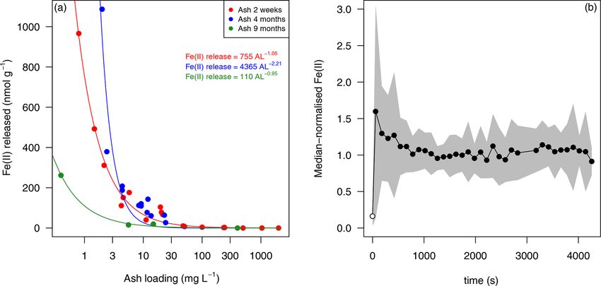
Ocean Sci., 17, 561–578, 2021 https://doi.org/10.5194/os-17-561-2021M. J. Vergara-Jara et al.: A mosaic of phytoplankton responses across Patagonia 571 Figure 7. Fe(II) release from Calbuco ash into seawater. (a) Mean Fe(II) released into South Atlantic seawater over a 30 min leach at 5–7 ◦ C. The same batch of Calbuco ash was subsampled and used to conduct experiments on three occasions after the 2015 eruption (2 weeks, 4 months and 9 months since ash collection). The lines are power law fits, with the associated equations shown in the legend. (b) The three time series of Fe(II) concentrations following ash addition are considered collectively by normalising the measured concentrations, such that 1.0 represents the median Fe(II) concentration measured in each experiment. All experiments were conducted for at least 30 min, those conducted with 4- and 9-month-old ash were extended for 1 h. The black line shows the mean response over 34 leach experiments with varying ash loading, and the shaded area shows ± 1 standard deviation. The initial Fe(II) concentration (pre-ash addition at 0 s) in all cases was below detection; thus, the detection limit is plotted at 0 s (open circle). Source data are provided in the Supplement (Table S2). phytoplankton community during the productive period due at two of three stations sampled could have resulted from to high light availability and high silicic acid supply, both ash fertilisation. However, if this was the case, it is not clear of which are influenced by freshwater runoff (González et which nutrient was responsible for this fertilisation, why the al., 2010; Torres et al., 2014). Therefore, the austral autumn bloom initiation occurred about 1 week after the third erup- season, encompassing the April–May 2015 ash deposition tive pulse (several weeks after the main eruption events) and events, is expected to have a high phytoplankton biomass the extent to which the timing was coincidental given that (Iriarte et al., 2007; León-Muñoz et al., 2018) which ter- productivity normally peaks in May. Reloncaví Fjord was to minates abruptly with decreasing light availability in austral the south of the dominant ash deposition from the 22 and winter (González et al., 2010). 23 April eruptions (Romero et al., 2016); thus, ash was de- Whilst not directly comparable, the magnitude of the 2015 livered by a mixture of vectors including runoff and rainfall. bloom in terms of diatom abundance (Fig. 4) was more in- The Petrohué River basin was particularly severely affected tense than that reported in Reloncaví Sound for 2001–2008. by ash with deposition of up to 50 cm of ash in places. This With respect to the timing of the phytoplankton bloom, the complicates the interpretation of the time series provided by low diatom abundances and chlorophyll a concentrations at high-resolution data (Fig. 3). With incident light also highly the end of May (Fig. 4) are consistent with prior observations variable over the time series (Fig. 3f), there are clearly sev- of sharp declines in primary production moving into June eral factors, other than volcanic ash deposition, which will (González et al., 2010). Peaks in diatom abundance were have exerted some influence on diatom and chlorophyll a measured at two stations on 14 May 1 week after the third abundance throughout May 2015. (small) eruptive pulse, and measured chlorophyll a concen- Primary production in the Reloncaví region is thought trations were highest close to station C on 30 April (Fig. 4). to be limited by light availability rather than macronutri- The high-resolution pH and O2 data collected at station C ent availability (González et al., 2010). Whilst micronutrient from mooring data are consistent with an intense phytoplank- availability relative to phytoplankton demand has not been ton bloom between ∼ 29 April and 7 May (Fig. 3), indicated extensively assessed in this fjord, with such high riverine in- by a shift to slightly higher pH and O2 during this time period puts across the region – which are normally a large source when river flow into the fjord was stable. of dissolved trace elements into coastal waters (e.g. Boyle Without a direct measure of ash deposition per unit area et al., 1977) – limitation of phytoplankton growth by Fe (or in the fjord, turbidity, or higher-resolution chlorophyll or di- another micronutrient) seems implausible. Reported Fe con- atom data, it is challenging to unambiguously determine the centrations determined by a diffusive gel technique in Relon- extent to which the austral autumn phytoplankton bloom was caví Fjord in October 2006 were relatively high: 46–530 nM affected by volcanic activity. The high abundance of diatoms (Ahumada et al., 2011). Similarly, reported dFe concentra- https://doi.org/10.5194/os-17-561-2021 Ocean Sci., 17, 561–578, 2021
572                                           M. J. Vergara-Jara et al.: A mosaic of phytoplankton responses across Patagonia

Figure 8. Potential biological impact of the 2015 Calbuco eruption observed via satellite remote sensing. (a–f) Spatial maps showing the
distribution of ash in the atmosphere (UV aerosol index) and corresponding images of chlorophyll a. Images were composited over 5 d
periods. Grey lines in the chlorophyll maps correspond to the UV aerosol index = 2 a.u. contour. (g, h) Time series of the UV aerosol index
and chlorophyll a for regions of the Pacific (g) and Atlantic (h) oceans, identified by boxes in the maps. Red vertical lines (22 April) indicate
the first eruption date. (i) Mean World Ocean Atlas surface NO3 concentrations. Thin black lines indicate the 500 m bathymetric depth
contour.

Ocean Sci., 17, 561–578, 2021                                                                     https://doi.org/10.5194/os-17-561-2021
M. J. Vergara-Jara et al.: A mosaic of phytoplankton responses across Patagonia                                                 573

tions in the adjacent Comau Fjord at higher salinity are gen-      than the simple Fe fertilisation proposed for the southeast Pa-
erally in the nanomolar range and remain > 2 nM even under         cific (Fig. 8g). In the absence of an immediate diatom fertili-
post-bloom conditions which suggests that dFe is not a lim-        sation effect from Fe or silicic acid, we hypothesise that any
iting factor for phytoplankton growth (Hopwood et al., 2020;       change in phytoplankton bloom dynamics within Reloncaví
Sanchez et al., 2019).                                             Fjord was mainly a “top-down” effect driven by the phys-
   Silicic acid availability could have been increased by ash      ical interaction of ash and different ecological groups in a
deposition. Whilst not quantified herein, an increase in sili-     nutrient-replete environment, rather than a “bottom-up” ef-
cic acid availability from ash in a region where silicic acid      fect driven by the alleviation of nutrient limitation from ash
was suboptimal for diatom growth could plausibly explain           dissolution.
higher than usual diatom abundance (Siringan et al., 2018).
Silicic acid concentrations were indeed high (up to 118 µM)        4.2   Volcanic ash as a unique source of trace elements
in Reloncaví Fjord surface waters and > 30 µM at 15 m
depth (salinity 33.4) (Vergara-Jara et al., 2019; Yevenes et       The release of the bio-essential elements Fe and Mn from
al., 2019). However, concentrations > 30 µM are typical dur-       ash here ranged from 53 to 1200 (dFe) and from 48 to
ing periods of high runoff and, accordingly, are not thought       71 nmol g−1 (dissolved Mn). For dFe, this is comparable
to limit primary production or diatom growth in this area          to the rates determined in other studies under similar ex-
(González et al., 2010). The Si(OH)4 : NO3 ratio in Relon-         perimental conditions for subduction zone volcanic ash,
caví Fjord and downstream Reloncaví Sound also indicates           with reported Fe release in prior work ranging from 2 to
an excess of Si(OH)4 , with ratios of approximately 2 : 1 ob-      570 nmol g−1 (Table S1 in the Supplement). For Mn, less
served in fjord surface waters throughout the year (González       prior work is available, but these values are within the 17–
et al., 2010; Yevenes et al., 2019). For comparison, the ra-       1300 nmol g−1 range reported by Hoffmann et al. (2012).
tio of Si : N for diatom nutrient uptake is 15 : 16 (Brzezinski,   Fe(II) release was particularly efficient at ash loadings
1985). Furthermore, experimental incubations with additions        < 5 mg L−1 (Fig. 7), whereas dFe release was less sensitive
of macronutrients to fjord waters in Reloncaví and adjacent        to ash loading (Fig. 6). The timing of Fe(II) release in the first
fjords have found strong responses of phytoplankton to addi-       60 s of incubations suggests a fast dissolution process. Fe(II)
tions of silicic acid only when Si(OH)4 and NO3 were added         is short-lived in oxic surface seawater with an observed half-
in combination, further corroborating the hypothesis that an       life of only 10–20 min even in the Southern Ocean where
excess of silicic acid is normally present in surface waters of    cold surface waters slow Fe(II) oxidation (Sarthou et al.,
these fjord systems (Labbé-Ibáñez et al., 2015). Therefore,        2011). However, relative to Fe(III), Fe(II) is also more sol-
it is doubtful that changes in nutrient availability from ash      uble and, from an energetic perspective, expected to be more
alone could explain such high diatom abundances in mid-            bio-accessible to cellular uptake (Sunda et al., 2001). Whilst
May.                                                               it is known that the vast majority of dFe leached from ash
   Alternative reasons for high diatom abundances in the           into seawater tends to occur in the first minutes of ash addi-
absence of a chemical fertilisation effect are plausible and       tion (Duggen et al., 2007; Jones and Gislason, 2008), and this
could include, for example, ash having reduced zooplank-           could be consistent with rapid dissolution of highly soluble
ton abundance or virus activity in the fjord, thereby facili-      phases on ash surfaces, we note that there is not yet conclu-
tating higher diatom abundance than would otherwise have           sive evidence concerning the precise origin of this dFe pulse.
been observed by decreasing diatom mortality rates in an           Fe(II) salts may be present on the surface of ash particles
environment where nutrients were replete. The role of vol-         (Horwell et al., 2003; Hoshyaripour et al., 2015); thus, the
canic ash in driving such short-term ecological shifts in the      Fe(II) observed herein (Fig. 7) may reflect almost instanta-
marine environment is almost entirely unstudied (Weinbauer         neous release following the dissolution of thin layers of salt
et al., 2017). However, volcanic ash deposition of 7 mg L−1        coatings in ash surfaces (Ayris and Delmelle, 2012; Delmelle
in lakes within this region during the 2011 Puyehue-Cordón         et al., 2007; Olsson et al., 2013). Alternatively Fe(II) could
Caulle eruption was reported to increase post-deposition           be released from more crystalline Fe(II) phases. Prior work,
phytoplankton biomass and decrease copepod and clado-              at much lower pH (pH 1 H2 SO4 representing conditions that
ceran biomass (Wolinski et al., 2013). The proposed mech-          ash surfaces may experience during atmospheric processing,
anism was ash particle ingestion negatively affecting zoo-         although not in aquatic environments) suggests that the short-
plankton, and ash-shading positively affecting phytoplankton       term release of Fe(II) or Fe(III) is determined by the surface
via reduced photoinhibition (Balseiro et al., 2014; Wolinski       Fe(II) : Fe ratio which may differ from the bulk Fe(II) : Fe ra-
et al., 2013).                                                     tio due to plume processing (Maters et al., 2017).
   Considering the more modest peak in diatom abundance               Different leaching protocols are widely recognised as a
at the most strongly ash-affected station (station A, Fig. 4)      major challenge for interpreting and comparing different
and the timing of the peak diatom abundance 3 weeks after          dissolution experiment datasets for all types of aerosols
the main eruption, it is clear that the interaction between ash    (Duggen et al., 2007; Morton et al., 2013). When Fe(II) is re-
and phytoplankton in the Reloncaví Fjord was more complex          leased into solution as a considerable fraction of the total dFe

https://doi.org/10.5194/os-17-561-2021                                                            Ocean Sci., 17, 561–578, 2021
You can also read