Impact of high-resolution sea surface temperature representation on the forecast of small Mediterranean catchments' hydrological responses to ...
←
→
Page content transcription
If your browser does not render page correctly, please read the page content below
Hydrol. Earth Syst. Sci., 24, 269–291, 2020
https://doi.org/10.5194/hess-24-269-2020
© Author(s) 2020. This work is distributed under
the Creative Commons Attribution 4.0 License.

Impact of high-resolution sea surface temperature representation on
the forecast of small Mediterranean catchments’
hydrological responses to heavy precipitation
Alfonso Senatore, Luca Furnari, and Giuseppe Mendicino
Department of Environmental and Chemical Engineering, Università della Calabria, P.te P. Bucci 42b,
87036 Rende (CS), Italy

Correspondence: Alfonso Senatore (alfonso.senatore@unical.it)

Received: 5 July 2019 – Discussion started: 16 July 2019
Accepted: 28 October 2019 – Published: 20 January 2020

Abstract. Operational meteo-hydrological forecasting             MER)/Centre European Remote Sensing d’Archivage et de
chains are affected by many sources of uncertainty. In           Traitement (CERSAT), which have a 24 h time resolution
coastal areas characterized by complex topography, with          and a 2.2 km spatial resolution. Precipitation estimates are
several medium-to-small size catchments, quantitative            compared with both ground-based and radar data, as well
precipitation forecast becomes even more challenging due         as discharge estimates with stream gauging stations’ data.
to the interaction of intense air–sea exchanges with coastal     Overall, the experiments highlight that the added value of
orography. For such areas, which are quite common in             high-resolution SST representation can be hidden by other
the Mediterranean Basin, improved representation of sea          more relevant sources of uncertainty, especially the choice
surface temperature (SST) space–time patterns can be             of the general circulation model providing the boundary
particularly important. The paper focuses on the relative        conditions. Nevertheless, in most cases, high-resolution SST
impact of different resolutions of SST representation on         fields show a non-negligible impact on the simulation of
regional operational forecasting chains (up to river discharge   the atmospheric boundary layer processes, modifying flow
estimates) over coastal Mediterranean catchments, with           dynamics and/or the amount of precipitated water; thus, this
respect to two other fundamental options while setting up        emphasizes the fact that uncertainty in SST representation
the system, i.e. the choice of the forcing general circulation   should be duly taken into account in operational forecasting
model (GCM) and the possible use of a three-dimensional          in coastal areas.
variational assimilation (3D-Var) scheme. Two different
kinds of severe hydro-meteorological events that affected the
Calabria region (southern Italy) in 2015 are analysed using
the WRF-Hydro atmosphere–hydrology modelling system              1   Introduction
in its uncoupled version. Both of the events are modelled
using the 0.25◦ resolution global forecasting system (GFS)       Operational river flood forecasting is a highly challenging
and the 16 km resolution integrated forecasting system (IFS)     activity for several reasons that go beyond strictly scien-
initial and lateral atmospheric boundary conditions, which       tific aspects. Hydrometeorological forecasting requires ex-
are from the European Centre for Medium-Range Weather            tremely complex systems, where issues like communication
Forecasts (ECMWF), applying the WRF mesoscale model              of warning, accessibility of the results, and administrative
for the dynamical downscaling. For the IFS-driven fore-          and/or institutional factors can be as important as monitor-
casts, the effects of the 3D-Var scheme are also analysed.       ing and modelling activities (Pagano et al., 2014; Silvestro
Finally, native initial and lower boundary SST data are          et al., 2017). Nevertheless, the cornerstone of such systems,
replaced with data from the Medspiration project by Institut     and undoubtedly the most demanding part from a scientific
Français de Recherche pour L’Exploitation de la Mer (IFRE-       point of view, is still the meteorological–hydrological mod-

Published by Copernicus Publications on behalf of the European Geosciences Union.
270                                                    A. Senatore et al.: Impact of high-resolution sea surface temperature

elling chain, supported by in situ or remotely sensed mea-         affected the location and intensity of high-impact events
surements.                                                         (Lebeaupin et al., 2006; Miglietta et al., 2011; Senatore et
   Increasingly refined modelling chains have been de-             al., 2014; Meredith et al., 2015; Pastor et al., 2015; Miglietta
veloped in recent years (e.g. UK Environmental Pre-                et al., 2017; Pytharoulis, 2018). Furthermore, using coupled
diction research, Lewis et al., 2019a; Canadian Great              atmosphere–ocean simulations, Berthou et al. (2014, 2015)
Lakes, Gronewold et al., 2011; the US Navy’s Cou-                  highlighted the major effects of long-term SST changes in the
pled Ocean/Atmosphere Mesoscale Prediction System                  representation of Mediterranean intense rain events, although
COAMPS® , Hodur, 1997). Despite their complexity, these            features at shorter timescales can also contribute signifi-
systems all have to deal with some inherent limitations of the     cantly. Lebeaupin et al. (2006) found that higher-resolution
meteorological and hydrological models. The main sources           SST fields have poor effects on convection in the case study
of errors in weather forecasts are connected to both inaccu-       they analysed (southern France). Ivatek-Šahdan et al. (2018),
racy in defining the initial state, due to the lack of available   examining several events in the eastern Adriatic, also found
measures or observation/assimilation errors, and approxima-        that more realistic SST fields did not substantially improve
tions of the models, whose structures are not capable of prop-     precipitation estimates; furthermore, they showed that the
erly representing the phenomena of interest (Allen et al.,         impact of high-resolution SST varied in different cases. Con-
2002; Buizza, 2018). These problems are exacerbated by the         versely, Katsafados et al. (2011) found noticeable deviations
chaotic nature of the atmosphere. Even though hydrological         among the forecast skills of simulations with SST boundary
models are much simpler than meteorological models with            conditions at different resolutions in a test case in the east-
respect to their structure (Liu et al., 2012; Pagano et al.,       ern Mediterranean, whereas Cassola et al. (2016) verified that
2014), they also have to struggle with different sources of        high-resolution SST fields can positively impact QPF in the
uncertainty that, according to Renard et al. (2010), can be        forecasting range of 36–48 h in a study in north-western Italy.
grouped into four categories: (1) input uncertainty, (2) output    Finally, Berthou et al. (2016), in southern France, and Stoc-
uncertainty (e.g. runoff estimates are not straightforward),       chi and Davolio (2017), in the Adriatic Sea, highlighted that
(3) structural model uncertainty, and (4) parametric uncer-        SST–atmosphere interactions mainly affect precipitation pat-
tainty. Furthermore, as catchments are very seldom perfect         terns and intensity via complex (and varying event-by-event)
natural systems, some effects of human disturbances can vir-       modifications of the stability of the upstream atmospheric
tually not be modelled.                                            boundary layer.
   The main link between atmospheric and hydrological                 The main objective of this paper is to contribute to the
compartments in a forecasting chain is precipitation fore-         current discussion on the impact of SST representation by
cast, which is an output variable for weather models and           extending the analysis over the whole meteo-hydrological
constitutes the main input for hydrological models. Quan-          forecasting chain, i.e. going beyond precipitation forecasts
titative precipitation forecast (QPF) is a major challenge for     and evaluating sensitivity on streamflow forecasts. Further-
operational meteorology, because the reliability of precipi-       more, SST sensitivity is assessed in the context of the over-
tation forecasts crucially affects streamflow forecasts’ skill     all uncertainty linked to initial and boundary conditions
(for a review see Cuo et al., 2011; for recent applications see    in regional modelling, using different forcing GCMs, with
e.g. Davolio et al., 2015, 2017; Tao et al., 2016; Li et al.,      and without data assimilation. To this aim, different ac-
2017). Among the various strategies adopted for addressing         curacy levels of SST representation are used in an opera-
this issue, in recent years, several studies that were focused     tional meteorological–hydrological forecasting chain over a
on coastal areas have assessed the importance of sea surface       coastal Mediterranean area including, in addition to the na-
temperature (SST) initial and boundary conditions as rele-         tive SST fields of the general circulation models (GCMs),
vant drivers of QPF, which, as previously stated, is conse-        higher-resolution fields: the Medspiration level 4 ultra-high-
quently capable of influencing the streamflow forecast. This       resolution foundation SST “SSTfnd” from the Medspiration
impact can be particularly strong in topographically com-          project by the Centre European Remote Sensing d’Archivage
plex coastal areas, characterized by several small catchments,     et de Traitement (CERSAT) and the Institut Français de
such as in the Mediterranean Basin, for which several co-          Recherche pour L’Exploitation de la Mer (IFREMER; Mer-
operative research efforts have been activated, including the      chant et al., 2008; Robinson et al., 2012). Furthermore, two
MEDiterranean EXperiment (MEDEX; Jansa et al., 2014)               GCM forecasts are used, namely the global forecasting sys-
and the HYdrological cycle in the Mediterranean eXperiment         tem (GFS) provided by the US National Weather Service
(HyMeX; Drobinski et al., 2018).                                   (NWS) and the integrated forecasting system (IFS) devel-
   Several studies have recently focused on the effects of         oped at the European Centre for Medium-Range Weather
sea surface–atmosphere interactions over heavy precipita-          Forecasts (ECMWF), as well as a three-dimensional varia-
tion at midlatitudes, particularly in the Mediterranean area       tional assimilation (3D-Var) scheme.
(e.g. Manzato et al., 2015; Romaniello et al., 2015; Rainaud          The study area, corresponding to the Calabrian Peninsula
et al., 2016). Some of them showed that large variations in        (southern Italy), due to its particular position in the middle of
the average values of SST boundary conditions significantly        the Mediterranean Sea and its complex and steep orography,

Hydrol. Earth Syst. Sci., 24, 269–291, 2020                                       www.hydrol-earth-syst-sci.net/24/269/2020/
A. Senatore et al.: Impact of high-resolution sea surface temperature 271
quite regularly experiences severe precipitation events and is relatively numerous recent events, this study focuses on two
particularly prone to significant ground effects (Federico et case studies that occurred in 2015 and were characterized by
al., 2003a, b, 2008; Chiaravalloti and Gabriele, 2009; Llasat distinctive features.
et al., 2013; Gascòn et al., 2016; Avolio and Federico, 2018), The first high-impact event (case study 1) was very lo-
the most recent of these (at the time of publication) be- calized in space and time and hit the north-eastern part of
ing a flash flood event on 20 August 2018 that caused 10 the region on the morning of 12 August 2015. The analy-
casualties (Avolio et al., 2019). According to Avolio and sis at the synoptic scale (Fig. 1a, b) shows that a main low-
Federico (2018), severe precipitation events over Calabria pressure system which originated from the Atlantic moved
can be classified as either short-lived events, which last less over the French and Spanish coasts in the early hours of
than 24 h, or long-lived events, which last more than 24 h. 12 August 2015, while a cut-off low occurred over the cen-
Following this classification, in this paper, two case studies tral Mediterranean, giving rise to a new low-pressure vor-
of events that occurred in 2015 are considered, the former tex with reduced dimensions that caused intense local rain-
is characterized by convective, very localized precipitation fall. The observed precipitation patterns (Fig. 1c) involved
(11–12 August; CFM, 2015a) and the latter by more per- only small areas of the mainland, specifically the Corigliano
sistent and widespread stratiform precipitation (30 October– and Rossano municipalities. The data provided by the Ital-
2 November; CFM, 2015b). ian national radar network (integrated into the same map
The meteorological–hydrological forecasting chain is in Fig. 1c), although underestimating ground observations,
based on the WRF-Hydro modelling system (Gochis et al., show that most of the precipitation occurred over the Ionian
2015). This open-source community model, originally devel- Sea. The Corigliano rain gauge measured high rainfall val-
oped as the hydrological extension of the Weather Research ues (Fig. 1d). During the 48 h from 00:00 UTC on 11 Au-
and Forecast (WRF; Skamarock et al., 2008) model, provides gust 2015 until 00:00 UTC on 13 August 2015, 255.2 mm
a coupling architecture that allows the user to connect ver- of rain was recorded, with a maximum of 246.4 mm in 24 h
tical water fluxes between the Earth surface and the atmo- (from 18:00 UTC on 11 August to 18:00 UTC on 12 Au-
sphere, which are simulated at coarse resolution by the at- gust), 223.2 mm in 12 h (from 01:45 UTC on 12 August to
mospheric model, to lateral surface and sub-surface fluxes, 13:45 UTC on 12 August), 167.4 mm in 6 h, 107.2 mm in
simulated at high-resolution by the hydrological model, in 3 h, and 51.4 mm in 1 h. The hydrological impact concerned
both a one-way (i.e. with no feedback from the routing mod- some small/very small coastal catchments, the most impor-
els to the atmosphere) and two-way (with feedback) manner. tant of which was the Citrea Creek (11.4 km2 – catchment
The WRF-Hydro system has dramatically evolved in recent boundaries highlighted in Fig. 1e), which overflowed caus-
years (Salas et al., 2018; Lin et al., 2018; Lahmers et al., ing several tens of millions of euros in damage.
2019), and has been operationally adopted into the NOAA The second event (case study 2) involved a much larger
National Water Model (NWM, Cohen et al., 2018) across the area and developed over 4 d, from 30 October to 2 Novem-
continental US, as well as being used for research applica- ber 2015. The synoptic analysis (Fig. 2e) shows another cut-
tions (e.g. Yucel et al., 2015; Senatore et al., 2015; Arnault et off low remaining stationary over Sicily for much of the pe-
al., 2016; Verri et al., 2017). riod and attracting humid and warm air from the Ionian Sea
The paper is organized as follows. Section 2 describes to the south-east (a detailed synoptic description of the event
the study area; the two events analysed; and the numerical is provided by Avolio and Federico, 2018). The orographic
model, including its set-up and details on the space and time effect in this event turned out to be decisive, with the Cal-
resolutions of the boundary conditions. In Sect. 3 the results abrian mountain ranges acting as a real barrier; therefore, a
of the meteorological and hydrological outputs are analysed large part of the rainfall occurred on the Ionian (eastern) side
separately for the two events. Finally, Sect. 4 discusses and of the region. While on 30 October 2015 only the northern
summarizes the main findings and outlines future research part of the region was affected (Fig. 2a; about 200 mm in 24 h
lines. at the Oriolo station), the highest precipitation during the en-
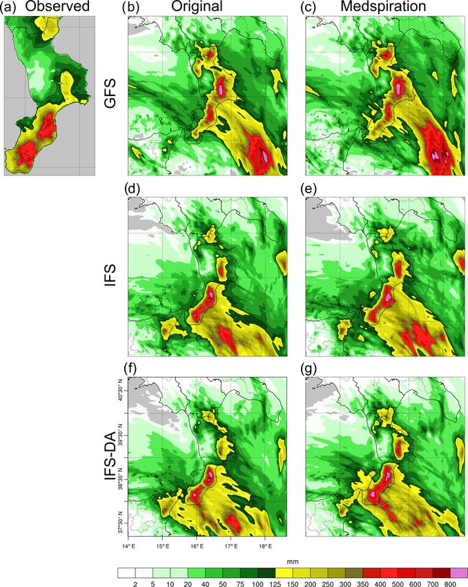
tire event was recorded on the southern coast (Fig. 2b, c, d),
with a maximum of about 740 mm (Chiaravalle Centrale sta-
2 Materials and methods tion) and a daily maximum of about 370 mm (Sant’Agata
del Bianco). In Fig. 2a–d, rain gauge observations over-
2.1 Study area and description of the events lap the precipitation fields detected by the weather radars,
also extending over the sea. The hydrological impact of the
Calabria is a peninsula characterized by a complex orogra- event concerned the whole eastern side of the region. Two
phy. Its geographical and morphological features produce a catchments are selected for this study, namely the Ancinale
very irregular precipitation distribution (average annual pre- River that is closed at the Razzona gauging station (116 km2 ,
cipitation varies between 600 and 1500 mm; Federico et al., Fig. 2f) and the Bonamico Creek that is closed at the Casig-
2010) and foster the occurrence of extreme weather events, nana gauging station (138 km2 , Fig. 2g). These catchments
which often caused deaths (Petrucci et al., 2018). Among the are chosen because they are two of the biggest with available
www.hydrol-earth-syst-sci.net/24/269/2020/ Hydrol. Earth Syst. Sci., 24, 269–291, 2020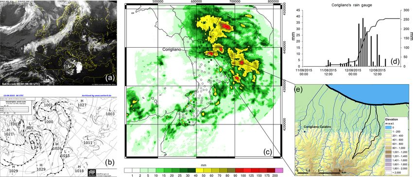
272                                                       A. Senatore et al.: Impact of high-resolution sea surface temperature

Figure 1. (a) Satellite images of the thermal infrared channel (10.8 µm) at 06:00 UTC on 12 August 2015 from http://www.sat24.com (last
access: 5 December 2019), © EUMETSAT. (b) Surface pressure and weather fronts at 06:00 UTC on 12 August 2015 from http://www1.
wetter3.de/ (last access: 5 December 2019), © Met Office. (c) Cumulative rain (mm) observed between 18:00 UTC 11 on August 2015 and
18:00 UTC on 12 August 2015; the points represent the weather stations, whereas spatially distributed values represent the radar estimation.
(d) Cumulative and hourly rainfall (mm) observed at the Corigliano rain gauge. (e) The Citrea Creek catchment, showing the location of the
Corigliano rain gauge.

water level observations (unfortunately no discharge data are           initial and lower boundary SST data are replaced by the
available), and they are located to the north and south of the          Medspiration L4 ultra-high-resolution SSTfnd (obtained as a
rainiest area, respectively. Specifically, Chiaravalle Centrale         daily mean with a resolution of 0.022◦ ). The high-resolution
station is located at the Ancinale River outlet.                        Medspiration SST fields are ingested into the WRF initial
                                                                        and lower boundary condition files of both domains via GIS-
2.2     Numerical model description and set-up                          based techniques, following Senatore et al. (2014).
                                                                           Furthermore, two relevant options allowed by the WRF
2.2.1    WRF                                                            modelling system are always activated for all SST bound-
                                                                        ary conditions: the sst_update option, allowing dynamical
The Advanced Research WRF (ARW) model, version 3.7.1,                   lower boundary (i.e. SST) conditions, and the sst_skin op-
is used in two one-way nested domains (Fig. 3). The ex-                 tion, based on Zeng and Beljaars (2005), which permits the
ternal domain, D01, covers a large area of the Mediter-                 simulation of SST dynamics. It is noteworthy that the higher
ranean (33.04–49.85◦ N, 3.59–28.59◦ E) with a 10 km (187×               resolution of the SST fields does not imply a greater accu-
205 grid points) horizontal resolution, whereas the inner-              racy, which can be objectively assessed via a comparison
most domain, D02, is centred over the Calabrian Penin-                  with in situ observations. For this purpose, a preliminary
sula (37.10–40.87◦ N, 13.88–18.71◦ E), with a 2 km (200 ×               search is performed in the Copernicus Marine Environment
200 grid points) horizontal resolution. The model runs on               Monitoring Service (CMEMS), in particular in the Corio-
44 vertical atmospheric layers, up to a 50 hPa pressure top             lis Ocean database for ReAnalysis (CORA; Cabanes et al.,
(about 20 000 m), and on 4 soil layers, down to 2 m below               2013), using the latest version (5.2, April 2019). Useful data
the surface. The time step of the model simulation is 60 s in           (i.e. continuous measurements with a sub-daily time step at
D01 and 12 s in D02.                                                    the sea–surface interface) are only found at the border of the
   Physical parameterization of the model is the same as that           external domain (D01) for both of the case studies (Fig. S1a
used by Senatore et al. (2014) and is reported in Table 1.              in the Supplement).
Boundary and initial conditions are provided by two oper-                  Finally, both as an additional comparison and with the aim
ational forecast GCMs, namely the GFS in forecast mode                  of highlighting its relative impact with respect to the effects
with a spatial resolution of 0.25◦ (about 27 km) and the high-          of different boundary conditions provided by different GCMs
resolution (HRES) IFS-ECMWF in forecast mode with a                     and/or more detailed SST fields, a data assimilation tech-
spatial resolution of about 16 km. In both cases, boundary              nique is also used for both of the test cases. Specifically, a
conditions are provided every 6 h. As a further step, both

Hydrol. Earth Syst. Sci., 24, 269–291, 2020                                              www.hydrol-earth-syst-sci.net/24/269/2020/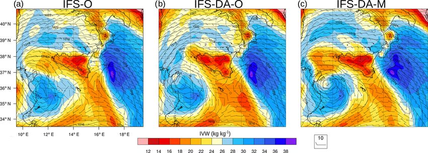
A. Senatore et al.: Impact of high-resolution sea surface temperature                                                                   273

Figure 2. Panels (a) to (d) represent the respective daily rainfall (mm) amounts observed from 30 October to 2 November 2015; the points
in these panels represent the weather stations, and the spatially distributed values represent the radar estimation. (e) Surface pressure and
weather fronts at 00:00 UTC on 1 November 2015 from http://www1.wetter3.de/, © Met Office. (f) Elevation maps of the Ancinale River
catchment and (g) the Bonamico Creek catchment.

Table 1. Main WRF physical options selected for the study.

                               Component                               Scheme adopted
                               Microphysics scheme                     Lin (Purdue) (Chen and Sun, 2002)
                               PBL scheme                              MJY (Mellor and Yamada, 1982)
                               Shortwave radiation physics scheme      Dudhia (Dudhia, 1989)
                               Longwave radiation physics scheme       RTTM (Mlawer et al., 1997)
                               Land surface model                      Unified NOAH (Tewari et al., 2004)
                               Surface layer                           Eta similarity (Janjić, 1994)
                               Cumulus physics scheme                  Kain–Fritsch (only D01) (Kain, 2004)

3D-Var assimilation scheme (Barker et al., 2004; Huang et                2.2.2   WRF-Hydro
al., 2009; Barker et al., 2012) is adopted, introducing con-
ventional meteorological observations into the initial condi-            In this work, WRF-Hydro version 3.0 is used in one-way
tions and adjusting boundary conditions to improve simula-               mode. Therefore, the atmospheric model outputs are used
tion performance.                                                        as input of the hydrological model utilizing an hourly time
   A summary of all of the simulations carried out is reported           step. According to the WRF parameterization, the land sur-
in Table 2.                                                              face model (LSM) is unified NOAH and is used at the same
                                                                         resolution as the D02 domain, whereas an increased horizon-
                                                                         tal resolution of 200 m is used (2000 × 2000 grid points) for

www.hydrol-earth-syst-sci.net/24/269/2020/                                                Hydrol. Earth Syst. Sci., 24, 269–291, 2020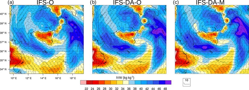
274                                                         A. Senatore et al.: Impact of high-resolution sea surface temperature

Figure 3. (a) The outer domain (D01) with a spatial resolution of 10 km; (b) the inner domain (D02) with a spatial resolution of 2 km.
Points 1 and 2 are considered when evaluating SSTSK (skin SST) evolution locally during the events according to different configurations
(Figs. 5 and 10 respectively). Vertically integrated water vapour fluxes are calculated across A–A’ and B–B’ (Figs. 9 and 13 respectively).

Table 2. List of simulations and their related acronyms.                rischi – ARPACAL, Calabria region). The interpolation tech-
                                                                        niques adopted are the same as those described in Senatore
       ID            GCM                       SST source               et al. (2015) except that precipitation fields are interpolated
       GFS-O         GFS 0.25◦ forecast        Original
                                                                        via inverse distance weighting (IDW) instead of exponential
       GFS-M                                   Medspiration             kriging. Furthermore, during the event (i.e. from 30 October
                                                                        to 2 November 2015) precipitation fields (Fig. 4a, b) are only
       IFS-O         IFS-ECMWF forecast        Original                 achieved by merging hourly ground-based rainfall observa-
       IFS-M                                   Medspiration             tions to hourly radar data estimates provided by the Italian
       IFS-DA-O      IFS-ECMWF forecast        Original                 weather radar network managed by the National Department
       IFS-DA-M      3D-Var assimilation       Medspiration             of Civil Protection. The merging procedure follows Sinclair
                                                                        and Pegram (2005) with the difference that a simpler double
                                                                        IDW interpolation method is used instead of a double kriging
                                                                        interpolation. The merging technique guarantees an increase
the lateral routing of surface and subsurface water; this re-           in the total “observed” rainfall volume of +4.6 % over the
sults in an aggregation factor of 1/10 from the atmospheric             Ancinale River and +10.6 % over the Bonamico Creek in
to the hydrological model.                                              comparison with a simple IDW interpolation.
   No observed discharge or flow depth data are available for              The parameters involved in the calibration procedure are
case study 1; therefore, model calibration is not performed.            broadly the same as those used in previous studies with
In case study 2, model calibration is performed manually                WRF-Hydro (e.g. Yucel et al., 2015; Senatore et al., 2015).
with respect to the available water level data for the two              Specifically, the LSM parameters calibrated are the infil-
selected catchments (Ancinale and Bonamico) with the aim                tration factor (REFKDT), the coefficient governing deep
of reproducing the timing of the hydrological responses to              drainage (SLOPE), and the thicknesses of the four soil lay-
heavy precipitation and, primarily, to correctly simulate the           ers. In addition, two spatially distributed parameters of the
peak flow time, which is a paramount variable for civil pro-            hydrological model, namely the overland flow roughness
tection activities.                                                     scaling factor (OVROUGHRTFAC) and the initial retention
   The humidity and temperature conditions in the four soil             height scaling factor (RETDEPRTFAC), are calibrated along
layers at the beginning of the analysed event (30 Octo-                 with the Manning roughness coefficients (one value for each
ber 2015 at 00:00 UTC) are achieved using offline simula-               stream order).
tions with a spin-up time of 1 month. The meteorological                   The calibrated parameters are shown in Table 3, whereas
forcing for this period is basically given by the spatial inter-        resulting hydrographs and uncalibrated hydrographs are
polation of ground-based observations (provided by the mon-             shown in Fig. 4c and d. The more impulsive behaviour of
itoring network managed by the Centro Funzionale Multi-                 the Bonamico Creek, typical of Calabrian “fiumare”, is sim-

Hydrol. Earth Syst. Sci., 24, 269–291, 2020                                             www.hydrol-earth-syst-sci.net/24/269/2020/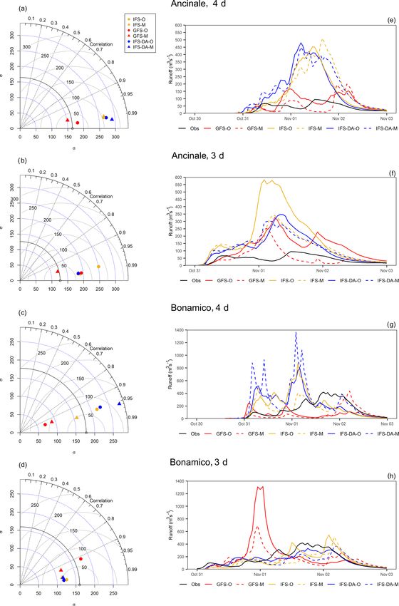
A. Senatore et al.: Impact of high-resolution sea surface temperature                                                              275

Figure 4. (a) Observed hourly rainfall (mm) averaged over the Ancinale River catchment; (b) as in panel (a), but for the Bonamico Creek
catchment. (c) A comparison between observed hydrometric levels (m) with respect to uncalibrated and calibrated simulated flow (m3 s−1 )
over the Ancinale River catchment; (d) as in panel (c), but for the Bonamico Creek catchment.

Table 3. Calibrated parameters of the offline WRF-Hydro model for       h is the water level, and a and b are the two calibration coef-
the Ancinale River and the Bonamico Creek.                              ficients) the coefficients of determination (R 2 ) between sim-
                                                                        ulated discharge values and observed water levels are equal
 Parameter                                        Ancinale   Bonamico
                                                                        to 0.942 and 0.831 for the Ancinale River and the Bonamico
 REFKDT                                                0.7        0.4   Creek respectively. Concerning the reliability of the simu-
 SLOPE                                                0.30       0.30
                                                                        lated discharge amount, as reference observations are miss-
 Z1 (m)                                                0.2        0.1
 Z2 (m)                                                0.5        0.2   ing, an indirect validation of the peak flows achieved is per-
 Z3 (m)                                               1.20        0.5   formed using the Hydrologic Engineering Center’s (CEIWR-
 Z4 (m)                                                  2        0.9   HEC) River Analysis System (HEC-RAS) (Hydrologic En-
 OVROUGHRTFAC                                           50         50
 RETDEPRTFAC (mm)                                        0         15
                                                                        gineering Center, 2016). Cross-sections for both of the out-
 The Manning roughness coefficient first order         0.1        0.1   lets of the catchments and for four upstream and downstream
 The Manning roughness coefficient second order      0.062      0.063   points, approximately 50 m apart, are determined by merg-
 The Manning roughness coefficient third order       0.048      0.045   ing data from an ultra-high-resolution (5 m) digital terrain
 The Manning roughness coefficient fourth order      0.033      0.031
                                                                        model provided by the Calabria Region Cartographic Centre
                                                                        with the heights given in very recent official maps (Technical
                                                                        Cartography of Calabria Region) at a scale of 1 : 5000. Such
ulated using lower values of the infiltration factor and lower          cross-sections are further validated by field sample measure-
soil layer thicknesses. Nevertheless, in order to allow timely          ments. One-dimensional steady flow simulations reaching
simulation of peak flows, a small delay of the initial re-              observed peak heights provide peak discharges broadly com-
sponse is necessary via an increase in the RETDEPRTFAC                  parable to the results achieved with the model.
value, which is compatible with noteworthy initial pond-                   For the sake of brevity, hereafter the WRF-Hydro hydro-
ing in the wide alluvial bed and infiltration in the gravelly           graphs calibrated using observed precipitation fields (shown
soil. Conversely, the abundance of organic matter in the soils          in Fig. 4) will be referred to as “observed hydrographs” or
of the dense forests within the Ancinale River catchment,               simply “observations”.
which (especially in autumn) can store considerable quan-
tities of water, most probably contributes substantially to the
smoother response of the Ancinale River. Figure 4c and d                3     Results and discussion
highlight that the calibration procedure mainly influences the
results for the Ancinale River, especially in terms of total vol-       3.1    Case study 1
umes.
    As for the hydrographs, adopting typical stage–discharge            The analysis with the CORA database (Fig. S1b–d) shows
power relationships (i.e. q = a · hb , where q is the discharge,        that Medspiration-derived lower boundary conditions, al-

www.hydrol-earth-syst-sci.net/24/269/2020/                                              Hydrol. Earth Syst. Sci., 24, 269–291, 2020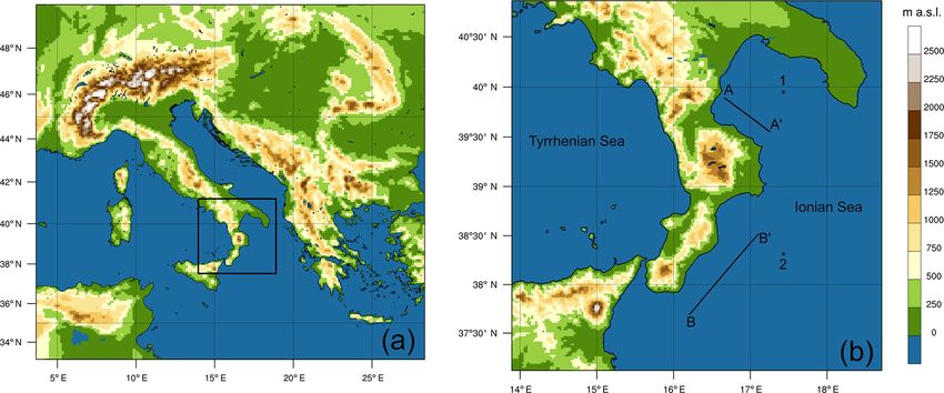
276                                                    A. Senatore et al.: Impact of high-resolution sea surface temperature

though originating from a high-resolution dataset, do not pro-     and IFS), but are centred more to the south. IFS-based simu-
vide a clear improvement of skin SST representation com-           lations forecast rainfall clusters with more elongated shapes
pared to the original GCM fields. It is to be noticed, how-        in the south–north direction, allowing more precipitation to
ever, that the SST boundary conditions in D01 are aggre-           reach the central and northern Ionian coasts (namely, the
gated at a 10 km resolution. Panels in Fig. S2 focus on D02        Corigliano-Rossano area). Even though simulations based on
and show the skin SST fields from 11 August at 18:00 UTC           the 3D-Var scheme still miss the correct location of the event,
to 12 August at 18:00 UTC with a time step of 6 h, for all         they both provide more rainfall in the domain (average values
simulations carried out in this case study. The main features      of 11.2 mm with the native SST fields and 11.0 mm with the
highlighted by the skin SST maps are the strong underes-           Medspiration SST fields) and also show a well-defined rain-
timation of native IFS fields close to the coastline (this is      fall cluster close to the central Ionian coast. Both IFS and 3D-
due to a known interpolation problem along coastlines that         Var simulations overestimate land precipitation in that area.
lowers temperatures to unrealistic values; Linus Magnusson,           According to the generally small differences identified in
personal communication, 2019) and the overestimation, es-          the SST fields, Fig. 6 clearly shows that ingesting high-
pecially in the Tyrrhenian Sea (up to more than 2 K), of the       resolution SST information provides (in terms of spatial
native GFS fields. The other skin SST fields mostly differ by      distribution of accumulated precipitation) much less rele-
less than ±0.5 K from each other. It is noteworthy that skin       vant (and partially chaotic) effects than changing initial and
SST fields in the simulations using the Medspiration prod-         boundary conditions or using data assimilation schemes, and
uct are not identical due to the fact that, with the method of     a minor or possibly opposite impact on the accuracy of
Zeng and Beljaars (2005), skin SST values are influenced by        the simulations. Given the peculiar features of the analysed
the surface winds and net radiation fluxes modelled by the         event, it makes sense to focus on the area surrounding the
different simulations.                                             Corigliano gauge station. For each simulation, the graph in
   A comparison of the time evolution of the average skin          Fig. 7a merges intensity, location, and time correlation in-
SST values in the whole D02 domain would be biased by              formation of the closest rainfall peaks (with a threshold of
the non-negligible IFS underestimation near the coastline.         at least 40 mm) to that station, whereas Fig. 7b explicitly
Instead, an analysis performed on selected significant points      shows the time evolution of accumulated rainfall for each
could provide more interesting insights. For this reason, fo-      of the locations identified (the points are highlighted using
cusing on the Ionian Sea, in Fig. 5, point 1, which is closer to   small stars in the panels of Fig. 6). Given that all simula-
Corigliano-Rossano, and point 2, which is off the Calabrian        tions strongly underestimate the observed rainfall value of
southern coast (the exact location of both points is given in      246.4 mm (the highest simulated value of about 100 mm is
Fig. 3b), are examined. Concerning daily values, a clear but       given by IFS-DA-M), there is no configuration clearly out-
slight (< 0.5 K) overestimation of GFS-O is shown for both         performing the others. Both GFS peaks are located to the
days in point 1 and on the second day in point 2. Some             south (about 20 km) and delay the rain event by 8 (GFS-
hourly differences are more evident: e.g. in point 1 GFS-O         M) to 11 (GFS-O) hours. IFS-O and IFS-DA-O peaks are
values are up to 1.5 K higher than other models on 12 Au-          lower than IFS-M and IFS-DA-M, but they are generally
gust at around 12:00 UTC, whereas in point 2 peak values           closer to the Corigliano station (about 13 and 22 km respec-
of IFS-O and IFS-M on 11 August at around 12:00 UTC are            tively). Furthermore, Fig. 7b shows that ingesting Medspira-
about 1 K higher than other models. Nevertheless, the differ-      tion fields moves the rainfall events up for both IFS-O and
ences among models during the night between 11 and 12 Au-          IFS-DA-O. This suggests that removing the unrealistic low
gust (i.e. right before and during the rain event) are generally   SST values along the coastline near Corigliano station (i.e.
low. The only noteworthy difference is given (in point 2) by       considering IFS-M and IFS-DA-M in place of IFS-O and
the small underestimation of Medspiration simulations (i.e.        IFS-DA-O respectively) has the twofold effect of increasing
GFS-M, IFS-M, and IFS-DA-M) of about 0.3–0.4 K, shown              rainfall amounts and accelerating flow dynamics. Such ef-
by a sudden reduction of their skin SST values, most prob-         fects are more easily recognizable looking at the 3D-Var sim-
ably due to the change of the Medspiration SST field (from         ulations, which provide more water vapour and precipitation.
11 to 12 August). This behaviour, which is clearly not realis-     Moving from IFS-O to IFS-DA-O to IFS-DA-M, the 850 hPa
tic, highlights a weakness occurring while directly ingesting      wind speed on 12 August at 00:00 UTC generally increases
such external data in the WRF simulation.                          in D02 and specifically off the northern Ionian coast of Cal-
   The accumulated precipitation modelled by all simulations       abria (Fig. S3). As a result, Fig. 8 shows that when moving
for the 24 h period from 11 August at 18:00 UTC to 12 Au-          from IFS-O to IFS-DA-O to IFS-DA-M, the integrated water
gust at 18:00 UTC is shown in Fig. 6. Overall, all models          vapour (IWV) cluster off the Ionian Sea simulated 3 h later
miss the location of the event, moving it further south, off       (03:00 UTC) is both larger and closer to the coast.
the Ionian coast. GFS-based simulations forecast more rain-           Differences between IFS-O and IFS-DA-O are due to the
fall than IFS-based simulations (average respective values in      assimilation of 14 vertical profiles of pressure, wind speed
the domain of 10.1 and 8.9 mm with the native SST fields and       and direction, absolute and dew point temperature, and rel-
10.4 and 9.5 mm with the Medspiration SST fields for GFS           ative humidity in D01, with 14 point measurements pro-

Hydrol. Earth Syst. Sci., 24, 269–291, 2020                                       www.hydrol-earth-syst-sci.net/24/269/2020/
A. Senatore et al.: Impact of high-resolution sea surface temperature                                                               277

Figure 5. Case study 1: temporal evolution of SSTSK (◦ C) at points 1 and 2, as shown in Fig. 3b.

vided by aircrafts at a fixed pressure level (corresponding             3.2   Case study 2
to about 12 km). In contrast, differences between IFS-DA-O
and IFS-DA-M are mainly due to different skin SST values.
Specifically, higher SST values given by ingesting Medspi-              Case study 2 embraces a longer period than case study 1. In
ration fields enhance water vapour concentration in the at-             this section, forecasting skills are assessed considering both
mosphere (the average upward moisture flux from the sea                 the whole 4 d length of the event (i.e. from 30 October 2015)
surface in domain D01 increases by about 5 %), while they               and a 3 d forecast starting on 31 October 2015, in order to
concurrently affect the stability of the atmospheric bound-             reduce the uncertainties attributable to the longer lead time
ary layer, providing more energy to the system and acceler-             forecast.
ating the flow dynamics (as reported by e.g. by Stocchi and                Such as in the previous case study, the first analysis is de-
Davolio, 2017). The early arrival of the moist air mass in              voted to skin SST fields. The comparison with the SST mea-
the Corigliano-Rossano area using Medspiration SST fields               surements available from the CORA database shows much
is highlighted by the time series of the hourly averaged wa-            better behaviour of the Medspiration SST fields in the anal-
ter vapour flux through section A–A’ (Fig. 9; section A–A’ is           ysed region of the external domain (Fig. S1e–g). Focusing on
shown in Fig. 3b). Local flow peaks are moved up from 2 to              the innermost domain, Fig. S4 highlights (besides the above-
4 h in advance using IFS-DA-M compared with IFS-DA-O,                   mentioned IFS-related problem along coastlines) that, in this
and similar behaviour, even though less evident, is observed            case, Medspiration fields for the whole period overestimate
with IFS-M compared with IFS-O.                                         both GFS and IFS native SST fields. Specifically, average
   Concerning the assessment of the hydrological impact of              differences with respect to GFS SST vary from about 0.6 to
the forecast event, notwithstanding the detailed analysis per-          0.8 K, whereas differences with respect to IFS SST fields are
formed, case study 1 does not provide relevant results (Ta-             higher than 0.8 K (the average difference increases to about
ble 4). The centre of the Citrea catchment is located approxi-          1.5 K if the values along coastlines are also considered). It
mately 8 km south-east of the Corigliano gauge station, has a           is noteworthy that GFS also underestimates skin SST par-
maximum length of about 7 km in the south–north direction,              ticularly near coastlines, whereas there is an overestimation
and a maximum width of only 2.5 km. The level of accuracy               off the Tyrrhenian Sea, such as that seen in the previous test
achieved by all simulations performed is not yet sufficient             case. Focusing on points 1 and 2 (Fig. 10), the following is
to correctly forecast the hydrological impact for such small            shown: (1) both points replicate similar general behaviour,
catchments in areas with very complex topography, such as               with Medspiration fields’ values being higher than values
those areas analysed in this study. The maximum rainfall ac-            from GFS, which, in turn, are higher than values from IFS;
cumulation value over the catchment is forecast by IFS-O,               (2) differences are more marked in point 1 (average values of
with 16 mm in 3 h. However, the accuracy of the models is al-           +1.0 and +0.6 K for IFS and GFS respectively) than in point
ready high enough to make them very useful (it is worthwhile            2 (+0.9 and +0.3 K for IFS and GFS respectively); (3) as in
recalling that the starting time of the simulation is more than         case study 1, a sudden reduction of about 0.5 K can also be
24 h before the event). In fact, if model forecasts are used            observed for Medspiration in the graph related to point 1,
to infer information about wider “warning areas” than single            moving from 1 to 2 November (Fig. 10a). Nevertheless, a
small catchments (as carried out by the Italian Civil Protec-           similar abrupt change, although less marked (about 0.2 K),
tion system), they provide essential inputs for civil protection        is observed also for GFS on 31 October at 06:00 UTC. In
activities.                                                             summary, this case study shows an evident skin SST increase
                                                                        from IFS to GFS to Medspiration.

www.hydrol-earth-syst-sci.net/24/269/2020/                                               Hydrol. Earth Syst. Sci., 24, 269–291, 2020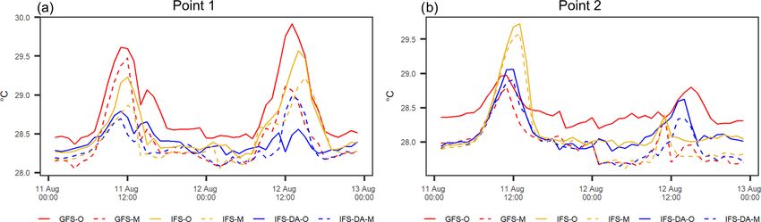
278                                                       A. Senatore et al.: Impact of high-resolution sea surface temperature

Figure 6. The 24 h accumulated precipitation (mm) from 18:00 UTC on 11 August 2015 to 18:00 UTC on 12 August 2015: (a) merged ground
measurements and radar observations simulated (b–g) using different configurations. The small blue (b–c) or white (d–g) stars highlight the
accumulated rainfall peaks near Corigliano, which are analysed in detail in Fig. 7.

Table 4. Accumulated rainfall between 02:00 and 08:00 UTC, and simulated peak flow and peak flow time in the Citrea Creek for the different
model configurations.

                                                        GFS-O     GFS-M      IFS-O    IFS-M     IFS-DA-O      IFS-DA-M
                 Accumulated precipitation between          0.0       0.7      15.8       5.3           1.1           1.4
                 02:00 and 08:00 UTC (mm)
                 Peak flow (m3 s−1 )                     0.005      0.002     0.132    0.048         0.006          0.006
                 Peak flow time (UTC)                       03         03        05       05            03             03

Hydrol. Earth Syst. Sci., 24, 269–291, 2020                                             www.hydrol-earth-syst-sci.net/24/269/2020/
A. Senatore et al.: Impact of high-resolution sea surface temperature 279
Figure 7. Circles in panel (a) are located at the peaks highlighted in Fig. 6 for each of the different configurations; the colours indicate the
time correlation, whereas the size refers to the percentage rain amount with respect to Corigliano observations. (b) Temporal accumulated
rainfall (mm) observed at Corigliano and simulated by the different peaks.
Figure 8. Column IWV (integrated water vapour; kg kg−1 , colour), sea level pressure (hPa; contours), and wind direction and speed (barbs)
at a height of 10 m at 03:00 UTC on 12 August 2015 for (a) IFS-O, (b) IFS-DA-O, and (c) IFS-DA-M respectively.
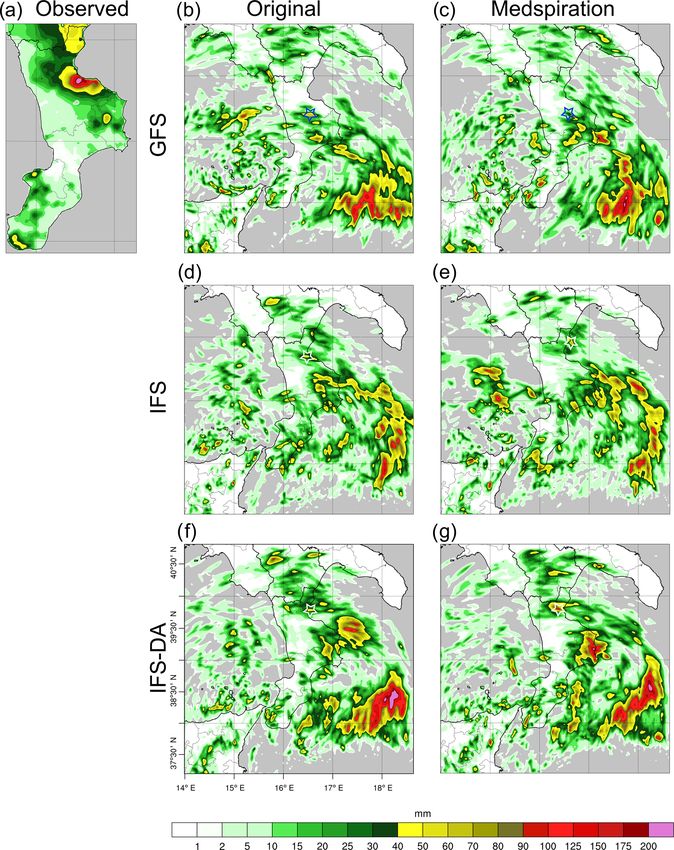
Figure 11 shows the accumulated rainfall fields in the 4 d
simulation period from the six WRF configurations com-
pared with a rainfall map of Calabria achieved by merging
ground measurements with radar observations (the merging
procedure followed Sinclair and Pegram, 2005; distinct rain
gauge and radar data are available in Fig. 2a–d). It clearly
highlights, in agreement with the previous case study, that
the main impact on rainfall output is given by the choice of
the GCM providing the boundary conditions. Average accu-
mulated precipitation in D02 is equal to 80 mm with GFS-
O, 71 mm with IFS-O, and 68 mm with IFS-DA-O. Interest-
ingly, the introduction of the 3D-Var scheme this time leads
Figure 9. Time evolution from 00:00 UTC on 11 August 2015 to to reduced precipitation (in D01, 22 vertical profiles and 16
00:00 UTC on 13 August 2015 of the vertically integrated water point measurements are assimilated). Higher skin SST val-
vapour flux (kg m−1 s−1 ) crossing section A–A’, shown in Fig. 3b. ues with Medspiration result in increased average precipi-
tation in D02 for all three cases, from +8 % (IFS-DA) to
+11 % (GFS). Concerning the precipitation patterns, for the
www.hydrol-earth-syst-sci.net/24/269/2020/ Hydrol. Earth Syst. Sci., 24, 269–291, 2020280 A. Senatore et al.: Impact of high-resolution sea surface temperature Figure 10. Case study 2: temporal evolution of SSTSK (◦ C) at points 1 and 2, as shown in Fig. 3b. Figure 11. Accumulated precipitation (mm) over the whole period of 96 h starting from 00:00 UTC on 30 October 2015: (a) merged ground measurements and radar observations; (b–g) simulated fields with the different configurations. Hydrol. Earth Syst. Sci., 24, 269–291, 2020 www.hydrol-earth-syst-sci.net/24/269/2020/
A. Senatore et al.: Impact of high-resolution sea surface temperature                                                          281

aims of this study, it is interesting to focus on the biggest        the event frequency, whereas ETS measures the fraction of
cluster in the south-east corner of the domain (i.e. the di-         correctly predicted events, adjusted for hits associated with
rection from which the humid air mass originates). Moving            random forecasts, and ranges from −1/3 to 1 (perfect score).
from GFS to IFS to IFS-DA, quite independently of the SST            Both scores are used for consecutive 6 h time intervals for
fields’ change, a shift of this cluster can be observed from         the analysed rainy period, utilizing precipitation thresholds
north-east to south-west.                                            with a step of 0.2 mm from 0.2 to 1 mm, a step of 1 mm up to
   The main change produced by the 3 d forecast compared             10 mm, a step of 2 mm up to 20 mm, and a step of 5 mm for
with the 4 d forecast is the higher correspondence of the GFS-       higher rates.
based simulations to the IFS-based simulations (Fig. S5).               Focusing on the 4 d simulations, ETS graphs show the gen-
The GFS-based rainfall footprints located in the south-east          erally better performance of IFS-DA-M, especially for higher
of D02 meet the Calabrian Ionian coast further south with            thresholds. Other models have conflicting levels of accuracy:
respect to the 4 d simulation, which is in agreement with the        e.g. IFS-DA-O is the best in Cala4, but the worst in Cala7.
IFS-based simulations. Overall, the simulated rainfall fields        Nevertheless, ingesting high-resolution SST generally pro-
are rather similar to each other and seem to reproduce the           vides better scores in all cases. Complementary information
observations in the southern part of the region reasonably           provided by FBI highlights a significant under-forecast of
well (i.e. the area most affected by the event), while the over-     GFS-based simulations in both Cala4 and Cala8 and an over-
forecast found in the 4 d simulation in the central zone is con-     forecast in Cala7. Other simulations behave better, but FBI
firmed. 3D-Var forecasts starting on 31 October assimilate 15        also points out that the 3D-Var scheme alone does not nec-
vertical profiles and 12 point measurements. Although the            essarily improve IFS-based forecasts (e.g. in Cala7 IFS-O is
IFS-based simulations forecast higher rainfall peaks off the         more accurate than IFS-DA-O), unless a high-resolution SST
southern Ionian coast (up to 1000 mm), the average accumu-           representation is also considered (IFS-DA-M always shows
lated precipitation in D02 is almost identical for all simula-       FBI values around 1). The ETS values of the 3 d simula-
tions (51 mm with GFS-O, 52 mm with IFS-O, and 53 mm                 tions are generally higher, but, in this case, the GFS-based
with IFS-DA-O). Precipitation increase caused by the higher          simulations are the worst, and introducing the Medspiration
skin SST Medspiration fields varies from +9 % (IFS-DA) to            fields further reduces their performance. Conversely, a more
+12 % (GFS), which is in agreement with the upward mois-             detailed SST resolution increases the ETS values of the IFS-
ture flux increase in D01 (+7 % with GFS, and +8 % with              based simulations in zones Cala4 and Cala8 (but not in zone
IFS and IFS-DA).                                                     Cala7). Concerning bias, FBI graphs show substantial under-
   With the aim of objectively assessing the performance of          forecasts in the Cala4 and Cala8 zones and an over-forecast
each WRF configuration, a detailed analysis using categor-           in the Cala7 zone. However, in this case, the GFS-based sim-
ical scores is carried out considering ground-based obser-           ulations provide better results, especially in Cala7 and for
vations in the civil protection warning areas more affected          high thresholds. Results achieved with ETS and FBI are gen-
by the event (grey areas in the reproduction of the Calabria         erally also confirmed by other scores (not shown), such as
region in Fig. 12). Specifically, 30, 19, and 22 rain gauges         the probability of detection (POD) score or the false alarm
are considered for the Cala4, Cala7, and Cala8 zones respec-         rate (FAR).
tively. Among the numerous scores available in the literature           As previously stated, higher skin SST Medspiration val-
(for a review see e.g. Wilks, 2006), for each zone Fig. 12           ues affect precipitation magnitude. This outcome agrees with
shows the results with respect to the frequency bias index           the average increase of upward moisture flux from the sea
(FBI),                                                               surface in D01 (+8 % with GFS, +13 % with IFS, and IFS-
                                                                     DA in the 4 d time period). Vice versa (and contrary to what
          hits + false alarms                                        was found in the previous case study), the simulations do not
FBI =                         ,                                (1)
             hits + misses                                           show relevant differences in the timing of the event. If the
and the equitable threat score (ETS),                                accumulated values of average precipitation in each of the
                                                                     warning areas are considered, all simulations are very highly
                      hits − hitsr                                   correlated (≥ 0.98, graph not shown) with observations. Fig-
ETS =                                          .               (2)   ure 13, showing the time series of hourly averaged water
          hits + misses + false alarms − hitsr
                                                                     vapour flux through section B–B’, highlights that there are
Here                                                                 no relevant forward nor backward time deviations between
                (hits + misses) (hits + false alarms)                the simulations with original skin SST fields and the corre-
hitsr =                                                    .   (3)   sponding simulations with Medspiration fields. The main ef-
          hits + misses + false alarms + correct negatives
                                                                     fect observed in Fig. 13 is the lower flux of the GFS-based
In the previous equations, the terms hits, misses, false alarms,     simulations because the main flow of soil moisture is shifted
and correct negatives refer to a typical 2 × 2 contingency           towards the north-east with respect to section B–B’ (in agree-
table. The FBI indicates if the forecast system has a ten-           ment with the precipitation maps in Fig. 11). The average
dency to underestimate (FBI < 1) or overestimate (FBI > 1)           flux increase with IFS-M and IFS-DA-M is about 3 %–4 %

www.hydrol-earth-syst-sci.net/24/269/2020/                                          Hydrol. Earth Syst. Sci., 24, 269–291, 2020
282 A. Senatore et al.: Impact of high-resolution sea surface temperature
Figure 12. Categorical scores ETS (equitable threat score) (a–f) and FBI (frequency bias index) (g–l) calculated on the rain gauges located
in the three civil protection warning areas more affected by the event from case study 2 (highlighted as grey areas on the map in the top left)
for both the 4 and the 3 d period.
SST Medspiration fields affects lower layers’ flow dynam-
ics, allowing more transport but not accelerating it. This be-
haviour can be attributed to the long-lasting characteristics
of the event that, developing at a wider scale than case study
1 and providing humid air continuously, smooths potential
differences in terms of timing.
Assessing the hydrological impact in the two selected
catchments is more interesting in this case study, because
all simulations forecast heavy rain over the catchment ar-
eas of the Ancinale River and Bonamico Creek, yet it is
still challenging because reliable hydrological forecasts re-
Figure 13. Time evolution of the vertically integrated water vapour
quire accurate QPFs at the catchment scale. A QPF perfor-
flux (kg m−1 s−1 ) crossing section B–B’ (shown in Fig. 3b) from
00:00 UTC on 30 October 2015 to 00:00 UTC on 3 November 2015. mance analysis is carried out for the catchment areas, con-
sidering the average values of the interpolated precipitation
fields. The simulated average precipitation over the Anci-
nale River catchment is strongly overestimated by all of the
compared with IFS-O and IFS-DA-O respectively. Figure 14, IFS-based simulations in the 4 d forecasts (from +53 % to
showing a snapshot of the IWV distribution in D01 during +72 %). Such over-forecasts are only partially reduced to
the event (31 October at 21:00 UTC), confirms the similar about +40 % (except for an increase to +80 % with IFS-
timing of the simulations. Moving from IFS-O to IFS-DA- O) in the 3 d forecasts. GFS-based simulations provide much
O to IFS-DA-M, the size of the cluster of humid air south of more reasonable biases in the 4 d forecasts (+12 % and −1 %
Calabria increases, but its position is basically the same. Sim- for GFS-O and GFS-M respectively), which are only par-
ilar conclusions are inferred from Fig. S6, which provides tially confirmed in the 3 d forecasts, where GFS-M pro-
additional information about 850 hPa wind fields in D02 at vides a nearly unbiased estimate (−3 %) but the GFS-O
the same time as in Fig. 14. over-forecast worsens to +44 %. Concerning the Bonamico
All simulations performed for this case study show that Creek catchment, in the 4 d forecasts the IFS-based biases
the greater energy supplied to the system by the higher skin
Hydrol. Earth Syst. Sci., 24, 269–291, 2020 www.hydrol-earth-syst-sci.net/24/269/2020/A. Senatore et al.: Impact of high-resolution sea surface temperature 283
Figure 14. Same as Fig. 8, but at 21:00 UTC on 31 October 2015.
are smaller in general (from −13 % to +22 %, but +54 % Furthermore, all simulations forecast the peak flows in ad-
with IFS-DA-M), whereas GFS-based simulations strongly vance compared with observations. Nevertheless, IFS-M,
under-forecast (−56 % and −43 % with GFS-O and GFS- IFS-DA-O, and IFS-DA-M show r values of around 0.6. In
M respectively). The 3 d bias is reduced for IFS-DA-based particular, IFS-DA-O (highest r value of 0.65) forecasts the
forecasts and slightly increased for IFS-based forecasts, with peak flow only 4 h in advance. Despite the good performance
values of around −20 % in all cases. GFS-based forecasts are with precipitation forecasts, the GFS-M hydrograph is not
much improved (+10 % and −16 % for GFS-O and GFS-M well correlated with observations and simulates the observed
respectively). The Taylor diagrams in Fig. 15a–d, based on peak flow about 9 h in advance. For Bonamico Creek, IFS-
the comparison of the average rainfall time series, generally DA-O results are even better (Fig. 15h). The simulated peak
show better performances of the GFS-based simulations in flow, according to precipitation forecasts, underestimates the
the Ancinale River and of the IFS-based simulations in the observed peak flow by about 20 %, but the correlation be-
Bonamico Creek. tween the simulated and observed hydrographs is high (0.89)
QPF analysis only partially reflects the main outcomes and the observed peak flow time (1 November at 16:00 UTC)
of the hydrological simulations, performed with the offline is delayed by only 2 h. Generally, all of the IFS-based simu-
WRF-Hydro model forced with the WRF downscaled fore- lations are well correlated (r values always higher than 0.6)
casts. According to precipitation over-forecast of the IFS- even though the peak flow time is always delayed (by up to
based simulations, both Fig. 15e and g (4 d simulations) 12 h). GFS-based simulations are poorly correlated and show
show a very relevant overestimation of all IFS-based hydro- significant overestimation and early forecast of the peak flow.
graphs (except IFS-M for Bonamico Creek). Nevertheless, in
the case of the Ancinale River, IFS-O, IFS-M, and IFS-DA-
M hydrographs are reasonably correlated with observations 4 Discussions and conclusions
(correlation coefficient, r, values of 0.62, 0.77, and 0.70 re-
Table 5 aims to support the discussion summarizing the main
spectively). Furthermore, simulated peak flow times of IFS-
outcomes concerning (1) the representation of the skin SST
O and IFS-M hydrographs are very close to the observed
fields; (2) the accumulated precipitation values in the internal
values, occurring on 1 November at 12:00 UTC (1 h before
domain and the related spatial distribution; (3) the time dis-
and 4 h after the observed peak flow respectively). The hy-
tribution of precipitation; and (4) hydrological impact (hy-
drographs resulting from GFS simulations are closer to ob-
drograph shape, total discharge, peak flow times), depend-
servations in terms of volumes; nevertheless, peak times are
ing on the GCM choice for determining the boundary con-
brought significantly forward in time or are delayed. Con-
ditions, the use of the 3D-Var scheme, and the use of the
cerning the Bonamico Creek, IFS-based hydrographs are not
high-resolution Medspiration fields.
well correlated and forecast peak flows are more than 12 h
in advance compared with observations, whereas GFS-based
hydrographs considerably underestimate flows.
The 3 d forecasts do not provide a substantial improve-
ment. The hydrological simulations over the Ancinale River
(Fig. 15f) are still affected by precipitation over-forecasts.
www.hydrol-earth-syst-sci.net/24/269/2020/ Hydrol. Earth Syst. Sci., 24, 269–291, 2020284 A. Senatore et al.: Impact of high-resolution sea surface temperature Figure 15. (a–d) Taylor diagrams related to the averaged hourly precipitation series over the Ancinale River catchment and the Bonamico Creek catchment simulated by the different configurations forecasting both 4 and 3 d, compared with observations. (e–h) The resulting hydrographs (m s−3 ) obtained by the different WRF-Hydro simulations compared with observations. Hydrol. Earth Syst. Sci., 24, 269–291, 2020 www.hydrol-earth-syst-sci.net/24/269/2020/
You can also read