Modelling habitat use suggests static spatial exclusion zones are a non optimal management tool for a highly mobile marine mammal

Marine Biology (2020) 167:62
https://doi.org/10.1007/s00227-020-3664-4

 ORIGINAL PAPER

Modelling habitat use suggests static spatial exclusion zones are
a non‑optimal management tool for a highly mobile marine mammal
Sarah L. Dwyer1 · Matthew D. M. Pawley1 · Deanna M. Clement2 · Karen A. Stockin1

Received: 18 July 2019 / Accepted: 4 February 2020
© Springer-Verlag GmbH Germany, part of Springer Nature 2020

Abstract
Understanding how animals use the space in which they are distributed is important for guiding management decisions in
conservation, especially where human disturbance can be spatially managed. Here we applied distribution modelling to
examine common dolphin (Delphinus sp.) habitat use in the Hauraki Gulf (36°S, 175°E), New Zealand. Given the known
importance of the area for foraging and nursing, we assessed which variables affect Delphinus occurrence based on gen-
eralised additive models (GAMs), and modelled probability of encounter. Behavioural information was included to assess
habitat use by feeding and nursing groups and determine whether persistent hotspots for such activities could be identified
and meaningfully used as a spatial management tool. Using data collected from dedicated boat surveys during 2010–2012,
depth and sea surface temperature (SST) were frequently identified as important variables. Overall, seasonal predictive
occurrence maps for the larger population resembled predictive maps of feeding groups more than nursery groups, suggest-
ing prey availability has important implications for the distribution of Delphinus in this region. In this case, static spatial
exclusions would not be the best management option as the core areas of use identified for these activities were large and
shifted temporally. It appears that at the scale examined, most of the Hauraki Gulf is important for feeding and nursing rather
than specific smaller regions being used for these functions. In cases where static management is not the optimal tool, as
suggested here for a highly mobile species, a dynamic approach requires more than a boundary line on a map.

Keywords Common dolphin · Delphinus · Predictive mapping · Species distribution modelling · Spatial management

 Introduction

 Understanding how animals use the space in which they are
 distributed is important for guiding management decisions
 (Guisan et al. 2013). Most studies of cetacean habitat use
Responsible Editor: V. Paiva.
 investigate the relationship between occurrence and envi-
Reviewed by J. M. Pereira and undisclosed experts. ronmental predictors over that of direct prey due to data
 availability (e.g., Panigada et al. 2008; Marubini et al. 2009;
S. L. Dwyer and M. D. M. Pawley contributed equally to the Garaffo et al. 2010; Santora 2011). For instance, cetacean
manuscript
 associations with environmental factors such as sea surface
Electronic supplementary material The online version of this temperature (SST) or chlorophyll concentration are often
article (https​://doi.org/10.1007/s0022​7-020-3664-4) contains classified as an indirect relationship, usually used as a proxy
supplementary material, which is available to authorized users. for prey distribution and concentration (Heithaus and Dill
 2002; Bräger et al. 2003; Cañadas and Hammond 2008;
* Sarah L. Dwyer
 s.l.dwyer@massey.ac.nz Azzellino et al. 2008; Dawson et al. 2013; Eierman and Con-
 nor 2014). Biological factors, such as group composition,
1
 Coastal‑Marine Research Group, School of Natural are also known to affect habitat use (Cañadas and Hammond
 and Computational Sciences, Massey University, North 2008; Guidino et al. 2014; Hartel et al. 2014; Melly et al.
 Shore, Private Bag 102904, Auckland 0745, New Zealand
 2017). Habitat use models help determine which environ-
2
 Cawthron Institute, 98 Halifax Street East, Nelson 7042, mental and/or biological variables may be more important
 New Zealand

 13
 Vol.:(0123456789)

62 Page 2 of 20 Marine Biology (2020) 167:62

to explain species’ distributions (Ferguson et al. 2006) and Common dolphins are subject to significant levels of tour-
serve as a predictive tool to aid conservation and manage- ism pressure in New Zealand, especially in the North Island
ment strategies (Cañadas et al. 2005; Silva et al. 2012; Red- where multiple operators with several vessels interact with
fern et al. 2013). the species in different core areas throughout the known
 Habitat heterogeneity and the biological requirements range of the species (Neumann and Orams 2006; Stockin
of a species interact to produce patterns in distribution and et al. 2008b; Meissner et al. 2015). In the Hauraki Gulf,
habitat use (Ballance 1992). Therefore, linking behaviour foraging has been shown to be significantly disrupted by the
to distribution enables a better understanding of the func- presence of tour boats, resulting in shorter foraging bouts,
tion behind any habitat use patterns (Norris and Dohl 1980; less time spent foraging overall, and more time required for
Hastie et al. 2004; Parra et al. 2006; Ribeiro et al. 2007). foraging dolphins to return to their initial behavioural state
This is important when attempting to manage populations (Stockin et al. 2008b). For Hauraki Gulf common dolphins,
exposed to human activities (Soldevilla et al. 2017; Tyne any adverse effects of local tourism might be compounded
et al. 2017) and can be critical for the establishment of con- for those individual dolphins that move between core areas
servation areas and management strategies (Cañadas et al. (Meissner et al. 2015; Hupman 2016) by increasing their
2005; Ashe et al. 2010). While static ocean management overall exposure to tourism. For this reason, protective
can be considered less challenging than dynamic protection measures have become necessary within the Gulf to miti-
(Maxwell et al. 2015; Pérez-Jorge et al. 2015), protected gate the risks of reduced feeding and nursing due to ongoing
areas need to be representative of species key biological tourism interactions.
functions (e.g., feeding and breeding habitats; Reeves 2000) The Department of Conservation is the regulatory body
but also follow shifts in the marine environment. Static man- responsible for the management of marine mammal spe-
agement will be ineffective if habitat use changes over time cies in New Zealand waters. Given the need for managers to
(Hartel et al. 2014). understand the local Hauraki Gulf area in terms of manag-
 Common dolphins (Delphinus spp.) are highly mobile ing the effects of tourism on common dolphins, but in the
and have a widespread global distribution, which is known absence of spatially explicit habitat data for Delphinus, this
to be affected by several environmental parameters such study examined common dolphin habitat use in the Hauraki
as depth, slope, and chlorophyll concentrations, that may Gulf. We used distribution modelling based on generalised
directly and/or indirectly affect prey distribution and con- additive models (GAMs) to identify important variables
centration (Hui 1979; Au and Perryman 1985). For example, affecting the occurrence of common dolphins in the inner
common dolphins occur in a range of water depths, using Hauraki Gulf (IHG) and in waters off the west coast of Great
shallow (< 100 m) waters in some locations such as the east- Barrier Island (GBI; i.e., outer Hauraki Gulf). Predictive
ern Ionian Sea in the Mediterranean (Bearzi et al. 2005) distribution models were then applied to make predictions
and the Gulf St. Vincent, Australia (Filby et al. 2010). In regarding the probability of encountering Delphinus in the
other areas, including the western Ligurian Sea in the Medi- IHG or off GBI, with the inclusion of behavioural infor-
terranean (Azzellino et al. 2008) and around the Azores in mation for feeding and nursery groups to further elucidate
the mid-Atlantic Ocean (Silva et al. 2014), they use deeper habitat use patterns. Given the known importance of the
pelagic waters (> 1000 m). Hauraki Gulf for feeding and nursing common dolphins
 In New Zealand, common dolphins have been recorded (Stockin et al. 2008a; Dwyer et al. 2016) and that common
around much of the coastline, with year-round presence dolphin presence in the Gulf is significantly affected by lati-
in some regions and only seasonal occurrence in others tude and water depth (Stockin et al. 2008a), we hypothesised
(Stockin and Orams 2009). However, both sighting and that persistent hotspots for these activities could be spatially
stranding data suggest this species is the most concentrated identified and meaningfully used as part of managed exclu-
off the northeastern coast of the North Island (Stockin and sion zones for tourism operations.
Orams 2009). The Hauraki Gulf region has been identified
as an important area for common dolphins (Stockin et al.
2008a; Dwyer et al. 2016), specifically for feeding (Stockin Materials and methods
et al. 2009) and nursing (Stockin et al. 2008a). Stockin et al.
(2008a) reported a high proportion of groups containing Study area
calves compared with other populations, and behavioural
analyses showed that common dolphins use the Hauraki Gulf The Hauraki Gulf (Fig. 1) is a relatively shallow, semi-
extensively for foraging (46.8% of the activity budget)— enclosed body of water on the northeast coast of the North
considerably more so than in other regions of New Zealand Island, New Zealand (Manighetti and Carter 1999; Black
such as the Bay of Plenty (17% of the activity budget) or et al. 2000). Circulation in the Hauraki Gulf is strongly
overseas (Stockin et al. 2009). influenced by surface winds and their interaction with tidal

13

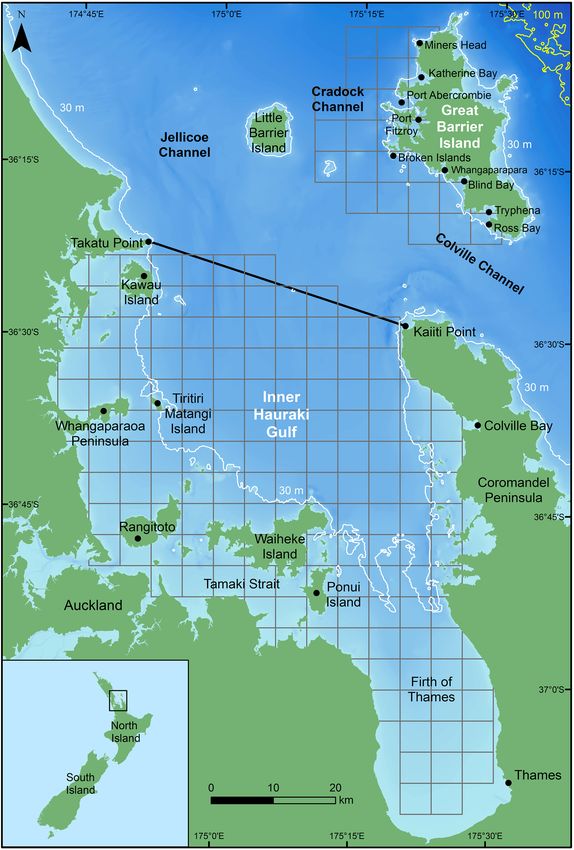
Marine Biology (2020) 167:62 Page 3 of 20 62

Fig. 1  The Hauraki Gulf, New
Zealand. The solid black line
(from Takatu Point to Kaiiti
Point) indicates the boundary
between the inner Hauraki Gulf
(IHG) and outer Hauraki Gulf
that includes Great Barrier
Island (GBI), the white lines
show the 30-m isobath and the
yellow lines the 100-m isobath.
Bathymetry is depicted with
darker shades of blue represent-
ing deeper waters; data courtesy
of NIWA (Mackay et al. 2012).
The 5 × 5-km grid is shown
in grey. Inset: Location of the
Hauraki Gulf, North Island,
New Zealand

currents, in addition to physical barriers such as headlands Two regions of the Hauraki Gulf were sampled in this
and islands that enhance local upwellings (Black et al. 2000). study, the IHG and GBI (Fig. 1). The dividing line between
Warm waters from the East Auckland Current (EAUC) flow inner and outer Hauraki Gulf waters was between Takatu
into the northerly entrance of the Hauraki Gulf during sum- Point and Kaiiti Point (Fig. 1). The IHG sampling area
mer and autumn when easterly winds and downwellings are included all waters south of the delineating line and cov-
more prevalent (Zeldis et al. 2004). Westerly winds that are ered 3480 km2. The 542 km2 GBI study site in the outer
favourable for upwellings prevail in late winter and spring Gulf mainly incorporated the coastal waters off the western
(e.g., Chang et al. 2003; Zeldis et al. 2004). side of the island, i.e., all waters between Miners Head in the

 13

62 Page 4 of 20 Marine Biology (2020) 167:62

north and Ross Bay in the south, up to a distance of 10 km in different behaviours (Stockin et al. 2009). Feeding groups
offshore (Fig. 1). were classified as all groups for which the initial behavioural
 state ‘forage’ was recorded. Nursery groups were defined
Data collection by the presence of at least one neonate. This conservative
 definition was selected rather than ‘groups that contained at
Sighting data were collected during dedicated monthly boat least one neonate and/or calf’, because calves are present in
surveys between January 2010 and November 2012 in the the Gulf year-round and are found in a high proportion of
IHG and between January 2011 and November 2012 off groups (Stockin et al. 2008a).
GBI. Surveys were conducted from a 5.5 m boat powered
by a 100 hp four-stroke engine when weather and sea con- Data analysis
ditions permitted. Survey design is described in detail in
Dwyer et al. (2016). In brief, time spent travelling along Sampling data
survey tracks actively searching for marine mammals was
classified as on effort. When the vessel left the survey track Grids of 5 × 5-km cells were created for the IHG and GBI
to approach dolphins, the survey mode switched to off effort study areas using ArcGIS version 10.0 (ESRI, Redlands,
until returning to the track to resume searching. Off effort California, USA; Fig. 1). All spatial data were processed
mode also included all other occasions when the vessel using ArcGIS and Geospatial Modelling Environment
was away from the survey track (e.g., returning to harbour (GME) version 0.7.2.0 (Beyer 2012), as per Dwyer et al.
because of deteriorating sea conditions or collecting data on (2016).
a sighting group). Surveys were conducted in conditions of Search effort was expressed as the number of kilometres
Beaufort sea state 3 or less and vessel speed was maintained of effort travelled through a grid cell per survey day. Beau-
at ~ 10 knots. fort sea state values were assigned to each 5 × 5-km grid
 When a common dolphin group was detected, the vessel cell for each sampling occasion (i.e., each time the vessel
left the survey track (i.e., off effort), approached to within track passed through a cell on a survey day). The value cor-
50 m of the group/individual, and commenced data collec- responded with the sea state recorded at the mid-point of the
tion. Water depth (± 0.1 m) was measured using an on-board vessel track within each grid cell.
depth sounder at the location of the group when first sighted. Only on effort sighting data were included in analyses.
All observational and environmental data were collected Any dolphin sighting(s) in a grid cell were denoted by a ‘1’
using an XDA Orbit II Windows Mobile device. Cyber- and an absence of sightings was denoted by a ‘0’. As such,
Tracker version 3 software (Steventon et al. 2002) was pro- a grid cell received a ‘1’ regardless of the number of sight-
grammed for logging observational data (e.g., behavioural ings (i.e., presence, maximum one per day). For the habitat
state) and to record the GPS position of the vessel every 60 s use models driven by behavioural traits, feeding and nursery
throughout the survey day. Beaufort sea state was logged at groups were assigned a ‘1’ and groups initially observed
15 min intervals. After observational data were recorded, the in other behavioural states or that did not include neonates
vessel returned to the survey route and resumed on effort to were assigned a ‘0’.
continue searching for further individuals/groups.
 Group composition (i.e., age class of individuals) and the Environmental data
initial behavioural state were visually assessed and recorded
for each encounter. A group of dolphins was defined as any The following environmental variables were considered to
number of individuals observed in apparent association, influence the distribution of common dolphins: depth, slope,
moving in the same general direction and often, but not tidal current, SST, and net primary productivity (NPP).
always, engaged in the same activity (Shane 1990). Age class These variables were selected because of their known effect
and behaviour definitions follow those previously described on common dolphin occurrence in the Hauraki Gulf (Stockin
for common dolphins using Hauraki Gulf waters (Stockin et al. 2008a) and other waters worldwide (e.g., Cañadas et al.
et al. 2008a, 2009, respectively). The initial behavioural state 2005; Cañadas and Hammond 2008; Moura et al. 2012).
of the group was assessed before the vessel reached within All were averaged at the 5 × 5-km grid level as follows: The
50 m. When determining the behavioural state, groups were mean depth (m) and slope (°) of grid cells were calculated in
scanned from left-to-right to ensure inclusion of all individu- ArcMap using the NIWA Hauraki Gulf bathymetric dataset
als in the group and avoid potential biases caused by specific (Mackay et al. 2012). Depth data for cells where dolphins
individuals or behaviours (Mann 1999). The behavioural were recorded (i.e., presence) were collected using the on-
state was determined as the category in which > 50% of indi- board depth sounder and within 100 m of the position of the
viduals were involved in, with all represented behaviours group when it was first sighted. For cells where dolphins
logged when an equal proportion of the group was engaged were not encountered (i.e., absence), depth was retrieved

13

Marine Biology (2020) 167:62 Page 5 of 20 62

 at the midpoint of the track segment in each cell surveyed with inshore coastal regions like the Hauraki Gulf that is
 using the NIWA Hauraki Gulf bathymetric dataset (Mackay surrounded by New Zealand’s largest city, Auckland, and
 et al. 2012). The mean maximum tidal current ­(ms−1) for features several estuaries and extensive coastal areas that
 each grid cell was extracted from the existing New Zea- are threatened by increased sediment runoff from the land
 land Marine Environment Classification raster ‘tidal_curr’ (Seers and Shears 2015).
 (https​://www.niwa.co.nz/coast​s-and-ocean​s/our-servi​ces/ The spatial variables considered for the models were east-
 marin​e-envir​onmen​t-class​ifica​tion), which was derived ing, northing, and distance to shore. Distance to shore (km)
 from a hydrodynamic model that simulated tidal current and was calculated using the ArcGIS near tool to measure the
 output the depth-averaged maximum tidal current (Snelder distance between the centroid of each grid cell and the near-
 et al. 2005). Daily SST data (°C) were obtained for the est point of land. If a cell centroid was located on land, the
 period of the study (i.e., from January 2010 to November distance to shore was classified as zero.
 2012) from the Physical Oceanography Distributed Active
 Archive Centre (PO.DAAC, NASA Jet Propulsion Labora- Models and predictions
 tory, Pasadena, California, USA; https​://earth​data.nasa.gov/
 about​/daacs​/daac-podaa​c) at a 1 km spatial scale and subse- Binomial GAMs (with logit link function) were used to
 quently averaged for each 5 × 5-km grid cell. The daily SST model the probability of encounter, where the response
data were used in the models and to calculate the monthly variable was a binary variable indicating sighting presence/
mean SST values for each region to examine SST patterns. absence within a grid cell. Models were chosen based on
The SST within-month standard deviation was calculated sensitivity and specificity calculated using Leave-One-Out
for each grid cell as a measure of variability that is expected cross-validation (LOOCV; details are described in steps 5
to be largest where strong oceanographic activity occurs in and 6 below). Separate datasets and models were used for
regions of strong spatial gradients or in regions of variable each of the following: (1) groups of common dolphins in
freshwater influence (Hadfield et al. 2002). NPP data (mg C the Hauraki Gulf (IHG and off GBI), (2) feeding groups
­m–2 day–1) were remotely collected (www.scienc​ e.oregon​ stat​ of common dolphins in the IHG, and (3) nursery groups of
 e.edu/ocean.​ produc​ tivit​ y) and based on the Vertically Gener- common dolphins in the IHG. The basic analytical workflow
 alised Production Model (VGPM; Behrenfeld and Falkowski is shown in Fig. 2 and described in detail below. All analyses
 1997). The VGPM is a model that estimates net primary were carried out using R version 3.5.3 (R Core Team 2014).
 production from chlorophyll using a temperature-dependent
 description of chlorophyll-specific photosynthetic efficiency. Step 1 Sub-sampling the data.
 NPP values were extracted as 8-day averages for each grid All data were highly unbalanced (with many more non-
 cell and NPP within-month standard deviation was also cal- occurrences (‘zeroes’) found than occurrences). Conse-
 culated. However, the NPP covariates were not included in quently, the dataset was reduced so it contained all occur-
 the models because NPP values could not be obtained for rences, but only an equivalent number of randomly selected
 all grid cells (mainly due to cloud cover, see Dwyer 2014) zeroes. In total, ten randomly sampled replicates of zeroes
 and there were concerns about reliable interpretation of the were used (in steps 1–5) for each dataset. This reduction in
 ocean colour data as chlorophyll algorithms do not perform zeroes served two purposes:
 accurately in waters where multiple co-existing, but not
 necessarily co-varying, dissolved and particulate marine 1. It sped-up model fitting, and
 and terrigenous substances affect ocean colour (Morel and 2. It greatly improved final model sensitivity (i.e., prob-
 Prieur 1977; Magnuson et al. 2004; Tzortziou et al. 2007; ability of correctly detecting an occurrence), albeit at
 Zheng and DiGiacomo 2017). This is typically associated the cost of lower specificity (correctly identifying those

Fig. 2  Workflow showing key steps used in each stage of analysis for any dataset

 13

62 Page 6 of 20 Marine Biology (2020) 167:62

 units without an occurrence). The number of zeroes was of the GAMs used thin-plate splines fit via restricted maxi-
 considered a hyper-parameter and tuned in step 3. mum likelihood (REML) within the R package ‘mgcv’
 (Wood 2017). Non-linearity was examined using component
Step 2 Develop an initial parsimonious model. plots, and, if the default smoothness appeared to overfit the
 The following were fit as covariates in the initial model: data, then flexibility was constrained by manually select-
year, season, northing, easting, depth, slope, distance to ing the number of knots. The GAM model fit covariates
shore, tidal current, SST, SST within-month standard devi- selected by the LASSO in step 2—this model was used to
ation, Beaufort sea state, and all meaningful interactions determine the sample size of zeroes that maximized the
among the variables. These variables were selected based True Skill Statistic (TSS; Allouche et al. 2006), i.e., the
on their hypothesised biological importance and the feasibil- sum of model sensitivity (how well the model predicted
ity of obtaining reliable measurements, with northing and occurrences) and specificity (how well it predicted zeroes)
easting included as proxies for unknown variables. The com- using LOOCV. For each model [i.e. (1) all, (2) feeding and
mon dolphin habitat model jointly modelled the occurrence (3) nursery group models], the number of zeroes randomly
of dolphins using data from both areas (IHG and GBI), but sampled was increased (from its initial value equal to the
area was examined as a possible covariate. Austral seasons number of occurrences) by 50 to determine if this improved
were defined as summer (December–February), autumn the TSS. For each sample size, the TSS was calculated by
(March–May), winter (June–August) and spring (Septem- building the model with all occurrences and each of the ten
ber–November) to allow comparisons with previous stud- random samples of zeroes. The sample size with the highest
ies conducted on common dolphins in the Hauraki Gulf average TSS (from the ten replicates) was determined to be
(Stockin et al. 2008a). The discrete nature of subset selection the optimal sample size (see step 5 for a description of how
methods (e.g., stepwise selection—where predictor variables TSS was calculated). Invariably, we found that increasing
are retained or dropped) is known to give biased standard the number of subsampled zeroes in the model decreased
errors, p values and regression coefficients and exacerbated sensitivity by more than the concurrent gain in specificity.
collinearity problems as well as highly variable models, i.e., So, in all models, the sample size of (randomly sampled)
small changes in the data may give very different models zeroes was the same as the number of occurrences—full
(Derksen and Keselman 1992; Breiman 1996; Tibshirani results are shown in Supplementary Table 1.
1996; Harrell 2001, Zou and Hastie 2005; Morozova et al.
2015). Consequently, we opted to use the LASSO (Least Step 4 Fitting GAMs.
Absolute Shrinkage and Selection Operator), a widely-used Variables were manually added (or removed) in an
model selection method (Heinze et al. 2018). The general attempt to improve the out-of-sample TSS values of the
idea of the LASSO is to reduce the residual sum of squares GAMs. Non-linearity was examined using component plots,
by adding a penalty term in the least squares objective func- and, if the default smoothness appeared to overfit the data,
tion that shrinks the coefficients towards zero. The penalty then flexibility was constrained by manually selecting the
term of the LASSO effectively adds a penalty term bias in number of knots.
an attempt to select a midpoint between high bias (overly Beaufort sea state was retained in all models because of
simplistic) models and high variance (overfitting to the train- its known effect on detecting cetaceans during field studies
ing data; Hastie et al. 2009). When the LASSO parameter, (e.g., Barlow et al. 1988; Gannier 2005) and by including it
λ, is small, the resultant coefficients are similar to ordinary as an explanatory variable, models could consider at least
least squares estimates. However, as λ increases, shrinkage some detection effects (Forney 2000). Similarly, effort was
occurs so that variables that are at zero are discarded. Conse- used as an offset in all models to account for the fact that
quently, a major advantage of LASSO is that it is a combina- more search effort is expected to yield more sightings.
tion of model regularization (i.e., reducing the likelihood of
overfitting) and a parsimonious selection of covariates. We Steps 5 and 6 Fitting and assessing candidate models.
implemented LASSO model selection using the R package Each candidate model was fit using the same ten replicate
‘glmnet’ (Friedman et al. 2010). The LASSO parameter, sub-sampled datasets (consisting of all presence data and the
which weights the penalty term and regularizes the model, ten replicate samples of zeroes). All candidate models are
was determined by choosing the value that minimizes the shown in Supplementary Table 2. Maximizing the average
prediction error rate using tenfold cross-validation (using the TSS was used as the basis for choosing the ‘best model’. TSS
default values in the function ‘glmnet::cv.glmnet()’. scores of each candidate model were based on out-of-sample
 model predictions determined using two components:
Step 3 Find the optimal sample size.
 A GAM using binomial distribution and logit link func- 1. Presence/absence of values within the sub-sampled data
tion was used to model occurrence. Non-linear components was predicted using LOOCV.

13

Marine Biology (2020) 167:62 Page 7 of 20 62

2. Absences that were not included in the sub-sampled data each grid cell that were used to create predictive maps using
 were predicted using a parameter set derived from fitting ArcGIS. Predictive values were not calculated for a small
 the entire sub-sampled data. Model parameter values number of grid cells as they were not sampled in all seasons
 using the entire sub-sampled dataset were used in all (IHG: n = 5; GBI: n = 3). These cells were not colour-coded
 tables presented in the results. and remained white on the predictive maps.

 In this manner, each candidate model had ten sets of pre-
dictions that were used to calculate ten values of TSS. Results
 Non-linear effects of covariates were graphically dis-
played showing how the probability of encounter varied Sampling data
when holding all other covariates constant at their mean
level (Beaufort level was held at zero, and, if the model also Survey effort totalled 279 d between January 2010 and
included a seasonal covariate, the effect assumed the season November 2012. A total of 887.6 h were spent on effort,
was ‘summer’). Confidence intervals (at the 50% and 95% totalling 16,786 km of on effort tracks within the IHG grid
levels) were calculated assuming asymptotic normality and cells. Between January 2011 and October 2012, 243.9 h
are also shown on these plots. were spent on effort in the GBI study area, with track effort
 Probability values for each grid cell were calculated at totalling 4017 km. Effort data are detailed further in fig. 2
the seasonal level (using seasonal averages for non-static and table 2 in Dwyer et al. (2016) and a map showing GPS
variables such as SST). The inverse link transformation was tracklines is presented in Supplementary Fig. 1. Although
used to obtain probability values on the scale of the original attempts were made to cover all areas homogeneously, effort
response variable since the results of the calculations were was not uniform across either study site (i.e., the 5 × 5-km
based on the scale of the linear predictor (Guisan and Zim- cells did not receive equal amounts of survey effort). For the
mermann 2000). For binomial GAMs, the inverse logistic IHG, 386 on effort dolphin sightings included 59 feeding and
transformation is 39 nursery groups; corresponding to 274 total, 52 feeding
 and 37 nursery group ‘grid cell sightings’ (i.e., presence
 exp (LP)
p (y) = , per grid cell per survey day). For GBI, 76 on effort dolphin
 1 + exp (LP) sightings included 12 feeding groups and 3 nursery groups;
 where LP is the linear predictor fitted by logistic regres- corresponding to 44 total, 6 feeding and 3 nursery group
sion. This transformation provided probability values for ‘grid cell sightings’.

Table 1  Parameter estimates of significant variables selected in the final common dolphin models for the inner Hauraki Gulf (IHG) and Great
Barrier Island (GBI; GAM with binomial distribution and logit link function)
Term Estimate SE Z value p value

Intercept 2.101 0.888 2.366 0.02*
Slope 3.014 1.761 1.711 0.09
SST – 0.876 0.184 – 4.765 < 0.001***
Depth-SST 0.017 0.004 3.968 < 0.001***
Slope-SST – 0.242 0.114 – 2.120 0.03*
Beaufort (1) – 0.502 0.365 – 1.375 0.17
Beaufort (2) – 0.639 0.335 – 1.905 0.06
Beaufort (3) – 0.769 0.391 – 1.969 0.05*
 edf 2 statistic p value

Current-Season (summer) 1.000 13.585 < 0.001***
Current-Season (autumn) 1.000 0.932 0.33
Current-Season (winter) 1.006 0.697 0.40
Current-Season (spring) 2.351 7.692 0.04*
Depth-Area (IHG) 2.894 25.590 < 0.001***
Depth-Area (GBI) 2.395 15.463 0.001**
% of deviance explained: 21.0

Interaction terms are denoted by (-); significance codes are ***0.001, **0.01, *0.05
edf estimated degrees of freedom

 13

62 Page 8 of 20 Marine Biology (2020) 167:62

Environmental data regions of increased slope mostly occurred in grid cells
 closer to shore, and the greatest tidal currents were adjacent
For the IHG, grid cells with deeper waters were located cen- to the Colville Channel and between Little Barrier and Great
trally and further north, while areas with increased slope Barrier Islands. These patterns are presented in Supplemen-
were observed close to shore (although not in southerly tary Fig. 2.
regions, e.g., Firth of Thames; Fig. 1). Regions with strong Mean monthly SSTs revealed that the coolest and warm-
tidal currents were apparent in the Firth of Thames, close to est water temperatures were experienced in August (IHG
the Colville Channel and in the channels between islands. 13.2 ± 0.2 °C; GBI 14.3 ± 0.3 °C) and February 2011
At GBI, water depths were greater for northern grid cells, (IHG 22.0 ± 0.1 °C; GBI 21.6 ± 0.1 °C), respectively. The

Fig. 3  Interaction between depth and sea surface temperature (SST) land. The black line is the average probability; shaded areas show
on the probability of encountering common dolphins in the inner one- and two-standard error intervals
Hauraki Gulf (IHG) and off Great Barrier Island (GBI), New Zea-

13

Marine Biology (2020) 167:62 Page 9 of 20 62

temperature range was smaller at GBI than in the IHG, cooler water temperatures, in areas of low to moderate tidal
where both the highest and lowest temperatures were current, increased slope, and generally in deeper waters (i.e.,
recorded. Waters also remained comparatively warmer at 30–50 m for the IHG and 50–80 m for GBI; Table 1, Figs. 3
GBI for longer in autumn and winter. During summer, GBI and 4). The exception was for GBI, where the probability of
inshore waters were cooler than IHG waters, especially com- encounter was predicted to be greatest in shallower waters
pared with western and southern regions of the IHG where (< 20 m) with SSTs lower than 13 °C (Fig. 3). Probability of
average temperatures were the highest. In winter, GBI waters encounter in areas with low currents was highly significant
were warmer than IHG waters, with average temperatures in summer (Fig. 4). Overall, the most significant variables
decreasing with increasing latitude. were SST, the depth-SST interaction, the effect of depth in
 the IHG, and the effect of current during summer (Table 1).
Habitat models Additionally, Beaufort sea state was a significant factor
 (Table 1), suggesting that the chances of encountering com-
Environmental variables that were frequently important in mon dolphins increased with calmer sea states.
the top habitat models were depth, slope, current, season Predictive maps indicated central northern regions of the
and SST. The chosen and candidate models are presented in IHG had the greatest probabilities of encountering dolphins
Supplementary Table 2. during all seasons, with higher probabilities in areas close to
 the 30-m depth contour in winter (Fig. 5). The overall prob-
Dolphin habitat use ability of encountering dolphins increased within the IHG
 over winter and spring when water temperatures were cooler
The final IHG and GBI common dolphin occurrence model (Fig. 5; Supplementary Fig. 3). Cells closer to shore also had
explained 21.0% of the deviance (Table 1). The model sug- increased probability values when SSTs were lower (Fig. 5;
gested that overall probability of encounter was greater in Supplementary Fig. 3). Use of the IHG remained relatively

Fig. 4  Interaction between tidal
current and season on the prob-
ability of encountering common
dolphins in the inner Hauraki
Gulf (IHG) and off Great Bar-
rier Island (GBI), New Zealand.
The black line is the average
probability; shaded areas show
one- and two-standard error
intervals

 13

62 Page 10 of 20 Marine Biology (2020) 167:62

Fig. 5  Predicted seasonal prob-
abilities of encounter for com-
mon dolphins in the Hauraki
Gulf, New Zealand. Red and
blue represent the highest and
lowest probabilities, respec-
tively, as shown in the probabil-
ity of encounter key. Black dots
show real sighting locations
from inner Hauraki Gulf (IHG)
surveys in 2010–2012 and Great
Barrier Island (GBI) surveys in
2011–2012. The 30-m isobath is
shown as a grey line

13

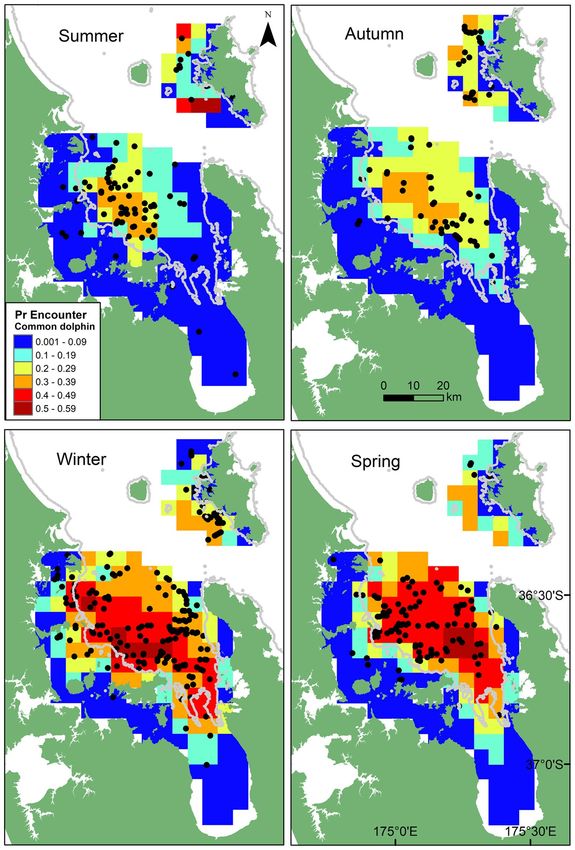
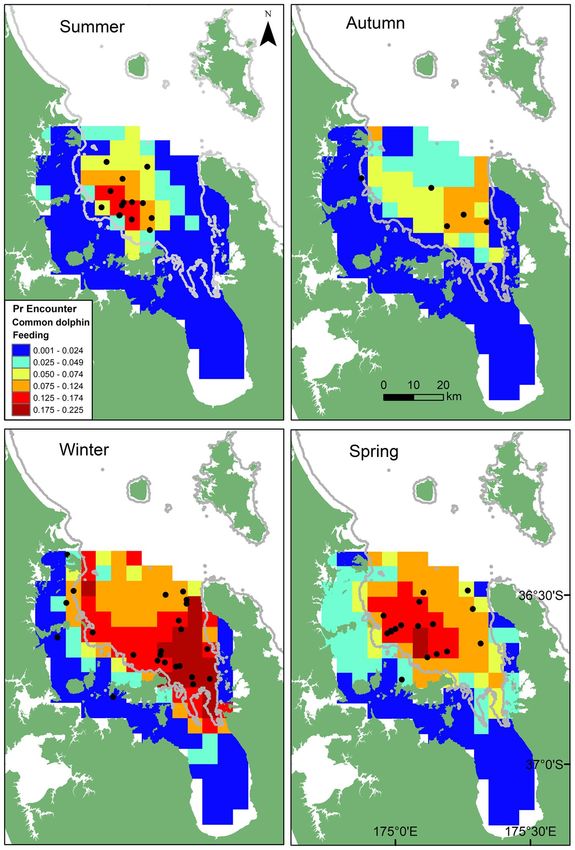
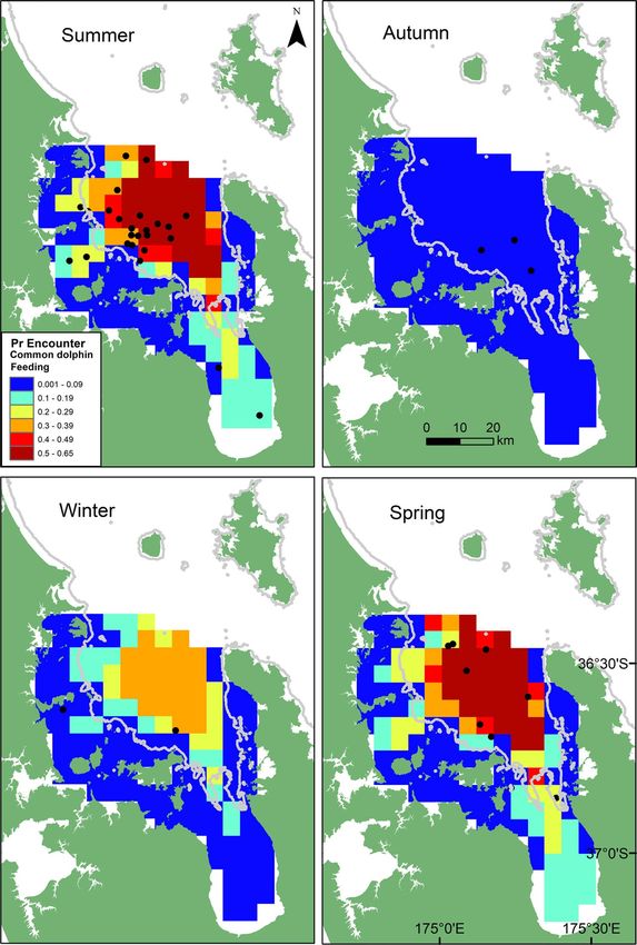
Marine Biology (2020) 167:62 Page 11 of 20 62

Table 2  Parameter estimates of significant variables selected in the final common dolphin model (GAM with binomial distribution and logit link
function) for feeding groups in the inner Hauraki Gulf (IHG)
Term Estimate SE Z value p value

Intercept 0.904 1.617 0.559 0.58
SST – 0.169 0.097 – 1.745 0.08
Beaufort (2) 0.521 0.538 0.969 0.33
Beaufort (3) 0.637 0.721 0.883 0.38
 edf 2 statistic p value

Depth-Season (summer) 1.839 5.905 0.08
Depth-Season (autumn) 1.000 3.450 0.06
Depth-Season (winter) 1.000 2.793 0.95
Depth-Season (spring) 1.000 6.014 0.01*
% of deviance explained: 18.1

Interaction terms are denoted by (-); significance codes are ***0.001, **0.01, *0.05
edf estimated degrees of freedom

low in autumn. At GBI, probability of encounter in northern Habitat use by nursery groups
and deeper regions was predicted greater in summer and
autumn, and greater in southern and shallower regions over The final nursery group model explained 43.0% of the devi-
winter (Fig. 5; Supplementary Fig. 2). ance (Table 3). Probability of encountering nursery groups
 declined significantly in autumn and increased in deeper
Habitat use by feeding groups waters and in areas of decreased slope (Table 3). The pre-
 dictive maps suggested that the probability of encountering
Very few sightings were made relative to the amount of nursery groups was greater within more central and northerly
effort for feeding or nursery groups in the GBI region; regions of the Gulf in spring and summer (Fig. 8). Beaufort
therefore, models were only fit for feeding and nursery sea state was also a significant factor suggesting the chances
groups in IHG waters. The final model for feeding groups of detecting a nursery group increased in calmer sea states.
explained 18.1% of the deviance (Table 2). The predictive
maps (Fig. 6) showed similar patterns to the overall dol- Hotspots for feeding and nursery groups
phin occurrence maps (Fig. 5), with a greater chance of
encountering feeding groups in northern and central regions Based on the predictive mapping, common dolphin use of
and increased probabilities in winter and spring compared the Hauraki Gulf was relatively widespread for both feed-
with summer and autumn when considering the full range ing and nursery groups. Both activities were predicted to
of depth categories. The overall probability of encounter- occur more commonly across central and northerly areas
ing feeding groups was predicted greatest in cooler waters, of the Hauraki Gulf, with the same general areas used
although this result was not significant (p = 0.08; Table 2). for both feeding (Fig. 6) and nursing (Fig. 8) functions.
Figure 6 showed that in general, winter and spring showed Therefore, the core areas of use that could be spatially
the highest probabilities of encounter in shallow water (note identified for these activities occurred over large spatial
the evidence of this relationship was only strong for spring), scales and shifted temporally (i.e., winter and spring for
with increased probability of encounter during summer at feeding groups, and summer for nursery groups). Spatially,
depths of approximately 40–50 m (Fig. 7). High probability it appears that most of the Gulf area is used for these func-
cells were more concentrated on the eastern side of the IHG tions rather than any distinctive smaller regions within
in winter compared with spring and summer (Fig. 6). the Gulf being important for feeding and nursery groups.

 13

62 Page 12 of 20 Marine Biology (2020) 167:62

Fig. 6  Predicted seasonal
probabilities of encounter for
feeding groups of common dol-
phins in the Hauraki Gulf, New
Zealand. Red and blue represent
the highest and lowest prob-
abilities, respectively, as shown
in the probability of encoun-
ter key. Black dots show real
sighting locations from inner
Hauraki Gulf (IHG) surveys in
2010–2012. The 30-m isobath is
shown as a grey line

13

Marine Biology (2020) 167:62 Page 13 of 20 62

Fig. 7  Interaction between
depth and season on the prob-
ability of encountering feeding
groups of common dolphins in
the inner Hauraki Gulf (IHG),
New Zealand. The black line is
the average probability; shaded
areas show one- and two-stand-
ard error intervals

Table 3  Parameter estimates of Term Estimate SE Z value p value
significant variables selected
in the final common dolphin Intercept 2.333 1.917 1.212 0.23
model (GAM with binomial
 Depth 0.047 0.030 1.562 0.12
distribution and logit link
function) for nursery groups in Slope – 8.210 2.666 – 3.079 0.002**
the inner Hauraki Gulf (IHG) Season (autumn) – 3.032 1.129 – 2.687 0.007**
 Season (winter) – 0.975 1.292 – 0.755 0.45
 Season (spring) – 0.052 0.799 – 0.065 0.95
 Beaufort (1) – 3.772 1.553 – 2.428 0.02*
 Beaufort (2) – 3.387 1.385 – 2.446 0.01*
 Beaufort (3) – 4.976 1.635 – 3.043 0.002**
 % of deviance explained: 43.0

 Significance codes are ***0.001, **0.01, *0.05

 13

62 Page 14 of 20 Marine Biology (2020) 167:62

Fig. 8  Predicted seasonal
probabilities of encounter for
nursery groups of common dol-
phins in the Hauraki Gulf, New
Zealand. Red and blue represent
the highest and lowest prob-
abilities, respectively, as shown
in the probability of encoun-
ter key. Black dots show real
sighting locations from inner
Hauraki Gulf (IHG) surveys in
2010–2012. The 30-m isobath is
shown as a grey line

Discussion to reduce exposure to human activity (e.g., Tyne et al. 2015).
 However, our analyses indicate that static spatial manage-
Disturbance to marine mammals from vessel interactions ment of common dolphins in the Hauraki Gulf would not be
and the associated effects (e.g., increased energetic demands, the optimal management tool to mitigate the known risks
acoustic disturbance, and reduced juvenile survival) are well of reduced feeding associated with ongoing tourism vessel
documented (Buckstaff 2004; Bejder 2005; Karpovich et al. interactions. This was evident by the absence of persistent
2015; Machernis et al. 2018). Spatial management, such as hotspots for feeding or nursery groups that could be mean-
restricting access to a habitat, is one tool often recommended ingfully used as part of managed exclusion zones.

13

Marine Biology (2020) 167:62 Page 15 of 20 62

 Our predictive mapping improves the current understand- waters, the probability of encounter increased during win-
ing of the spatial and temporal habitat use of the Hauraki ter and spring. Short-beaked common dolphins (D. delphis
Gulf by common dolphins and creates a baseline for spatial ponticus) in the Black Sea are known to move from off-
planning and decision making. However, our results come shore waters to shallow coastal waters to feed on Black Sea
with some limitations. Modelling the occurrence of mobile anchovy (Engraulis encrasicolus ponticus) and Black Sea
species inhabiting a highly dynamic environment is chal- sprat (Sprattus sprattus) in the winter and summer, respec-
lenging given the degree of random variability and the large tively (Reeves and Notarbartolo di Sciara 2006). A change
number of possible explanatory variables used to try to cap- in prey availability and/or their seasonal distribution within
ture the heterogeneity in environmental conditions. While Gulf waters may have also affected the change in common
some variables were highly significant for certain regions dolphin habitat use.
in this study, the explained deviances for two of the models Although the occurrence of clupeid fish such as pilchards
(the IHG/GBI and the feeding group models) were relatively and sprats (Harengula antipoda) has been documented as
low. Such results are often typical for this type of data (e.g., erratic and their migrations difficult to predict (Young and
Ferguson et al. 2006; Cañadas and Hammond 2008; Embling Thomson 1926), they have been described as locally abun-
et al. 2010) and have been attributed to factors such as the dant in some regions of New Zealand such as Wellington
spatial scale of the study area (Cañadas and Hammond 2008) harbour in winter and spring (Young and Thomson 1926;
or a mismatch in predictor variables used as proxies for prey Ministry for Primary Industries 2013). Changes in seasonal
distribution or abundance (Ferguson et al. 2006). For exam- abundance or movements of pilchards in the Hauraki Gulf
ple, our analyses may have been limited by not including a have not been assessed, as with other important species in
measurement for productivity in our models. As a result, the diet of common dolphins, such as jack mackerel (Tra-
spatial management tools such as spatial exclusion zones for churus spp.). However, limited fisheries catch data obtained
tourism operations can be affected by low levels of certainty from the Ministry for Primary Industries for the period of
associated with predictive models. this study show some alignment with the findings presented
 The environmental variables that were most frequently here, with a significant proportion of the annual pilchard
significant in the habitat models presented here were depth catch taken during the winter month of August (Dwyer
and SST. Depth was also identified as one of the most 2014). Baker (1972) suggested that minimum water tem-
important factors driving the spatial distribution of ceta- peratures of approximately 14 °C may be warm enough to
ceans in the Hauraki Gulf in a recent aerial survey study support year-round spawning of pilchards off northeastern
(Kozmian-Ledward 2014). Model results indicated that New Zealand. Such a consistent source of prey could explain
the greatest probability of encountering common dolphins the year-round use of the Hauraki Gulf by common dolphins,
within the IHG was during the colder months of winter and as suggested by Stockin et al. (2008a).
spring (when SSTs were lowest) and within deeper waters The inclusion of functional data into the models provided
(30–50 m), the latter consistent with a previous study of further information about habitat use of common dolphins
common dolphin occurrence (Stockin et al. 2008a). The in the Hauraki Gulf, as previously demonstrated by Cañadas
highest chances of encountering common dolphins off GBI and Hammond (2008) for short-beaked common dolphins in
was also in deeper waters (50–80 m) during warm SSTs; the southwestern Mediterranean. Feeding groups were pre-
but in shallow waters (< 20 m) during very low SSTs of dicted to occur more commonly in northern-central regions
13 °C. There did not appear to be any well-defined spatial of the IHG during winter and spring. These data correspond
trends in SST that could explain these patterns (see Supple- well with the results of an earlier (2002–2005) behavioural
mentary Fig. 3). It seems more likely that encounter prob- study that found most foraging common dolphins were found
abilities may be related to prey movements, i.e., that depth in the deepest waters of the IHG, and primarily during win-
is a proxy for prey distribution and/or location in the water ter and spring (Stockin et al. 2009). While feeding groups
column. For example, pilchard (Sardinops neopilchardus) were generally observed in deeper waters in this study, it
are known to be more abundant in bays and harbours in New was still possible to encounter a feeding group in shallow
Zealand when water temperatures are cooler (Ministry for regions, but only when SSTs were at their lowest. Overall,
Primary Industries 2013) and are also known to form com- the seasonal predictive occurrence maps for the larger popu-
pact schools particularly during the summer (Fisheries New lation resembled seasonal predictive maps of feeding groups
Zealand 2018). Both of these factors may help explain the more than nursery groups, suggesting prey availability likely
increased probability of encountering Delphinus in the IHG has important implications for the general distribution and
during the colder months but off GBI during the warmer habitat use patterns of common dolphins in the IHG.
months. Nursery groups in the IHG were most prevalent during
 Northern and central regions of the IHG were used year- summer, in line with other North Island studies (Stockin
round by common dolphins, while for shallow inshore et al. 2008a; Meissner et al. 2014) and common dolphin

 13

62 Page 16 of 20 Marine Biology (2020) 167:62

research conducted overseas (Cañadas and Hammond 2008). governed by processes at multiple scales (Dormann 2007).
The prediction for increased use of areas with similar water However, it seems unlikely that any potential identification
depths (~ 40 m) by nursery groups (Fig. 8) and the general of smaller hotspots would result in a recommendation for the
population (Fig. 5) is consistent with Meissner et al. (2015) use of spatial exclusion zones in this case given the tempo-
who also reported groups in similar water depths regard- ral shifts in intense use of the central and northern regions
less of group composition in the Bay of Plenty. However, of the Gulf. Moreover, any smaller hotspots would still be
these results differ to those reported by Stockin et al. (2008a) expected to be widely distributed across large areas of the
who found that groups including neonates were typically Gulf. Additionally, selecting a wider spatial extent [e.g.,
observed in shallow waters of less than 20 m depth. It is not northeastern North Island waters—for which movements of
clear whether the different observations represent a change common dolphins outside of the Hauraki Gulf are known
in habitat use over the period of the two studies or differ- (Hupman 2016)] may have identified the entire Hauraki
ences in survey methodologies. The latter seems less likely Gulf as the preferential area for the population, as previously
given that most of the data analysed in Stockin et al. (2008a) suggested (Dwyer et al. 2016). However, the aim of this
were collected from a tour vessel that spent more time in study was to investigate habitat use within the Gulf, given
deeper waters searching for whales, and thus presumably the extent and known effects of tourism within the region.
would have had more opportunities to encounter neonates in Following the results presented here, it would be prudent
deeper waters. Unfortunately, small sample sizes precluded to examine habitat use at such a wider scale to determine
the fitting of functional models for GBI to help elucidate the relative importance of Hauraki Gulf waters for common
these patterns further. dolphins and indeed other cetaceans.
 The predictive maps revealed relatively widespread use Visual surveys for cetaceans are known to be affected
of the central Hauraki Gulf for both feeding and nursery by imperfect detection; i.e., detection of groups/individuals
groups, albeit with temporal differences in use (feeding is rarely perfect (Bailey and Adams 2005). This is due to
groups most prevalent in winter and spring, and nursery factors such as sighting methods, sighting cues, search con-
groups most prevalent in summer). Spatial exclusion zones ditions, and group size (Barlow et al. 2001). While survey
for tourism operations would, therefore, be difficult to imple- protocols in the present study were kept consistent during
ment for these activities given the areas that were identified the entire sampling period to try to minimise factors affect-
as important were large, covering most of the areas used ing detection, and variables (Beaufort sea state and effort)
by common dolphins and consequently the tour vessels. As that were deemed to have significant effects on the detection
such, placing a large static spatial exclusion boundary the of cetaceans during boat surveys were incorporated into the
size of the area used by feeding and nursery groups would models, these variables did not account for detection prob-
not be the best management tool in terms of stakeholder ability explicitly or spatially. As such, the results we present
support or practicalities such as the ease of enforcement will underrepresent true levels of habitat use since imperfect
(Wilhelm et al. 2014). detection will result in negatively biased results (MacKenzie
 Our study used one spatial scale (i.e., 5 × 5 km grid cells et al. 2002). Nevertheless, the identification of high and low
within a combined 4022 km2 area of the Hauraki Gulf) use areas in this study is expected to be consistent whether
to assess habitat use. Previous studies have examined the detection probability was accounted for or not, as demon-
effects of different spatial scales on cetacean distribution and strated in Dwyer (2014) when assessing predictions of com-
habitat use with mixed results; for example Redfern et al. mon dolphin habitat use in the Hauraki Gulf based on both
(2008) did not identify significant differences in selected generalised linear models and occupancy models.
variables, their functional forms, or high and low-density In cases where the use of static management areas is not
regions of predictive maps when assessing different spatial the preferred tool, particularly for highly mobile species,
resolutions for dolphin habitat use in the eastern tropical other management priorities should be considered. Man-
Pacific. González García et al. (2018) examined high and agement options other than static spatial exclusion include
coarse spatial resolutions when investigating habitat pref- but are not limited to increased enforcement of regulations,
erences of Azorean blue whales (Balaenoptera musculus), reassessment of permissible viewing distances and ves-
reporting that both scales were valid and beneficial for cap- sel speeds, and temporal closures (Machernis et al. 2018).
turing larger oceanographic features (coarse resolution) and Dynamic ocean management (i.e., management that rapidly
more localised short-term events (high resolution). Con- changes in space and time in response to changes in the
versely, Scales et al. (2017) assert that the use of coarse- ocean and its users) has also been proposed as a promising
scale data risks significant predictive inaccuracy in habitat tool that allows for near-real-time adjustments to conserva-
models. It cannot be ruled out that using a finer resolution in tion strategies (Maxwell et al. 2015; Abrahms et al. 2019).
our study may have identified several smaller distinctive core Hazen et al. (2018) demonstrate that dynamic closures of
areas of use given that species distribution patterns may be the California drift gillnet fishery could be up to ten times

13

Marine Biology (2020) 167:62 Page 17 of 20 62

smaller than existing static closures while simultaneously feeding groups that could be identified from the predictive
supporting fishing opportunities and maintaining adequate mapping were large and shifted temporally. Therefore, we
protection of endangered nontarget species. Examples of suggest that spatial exclusion zones would not be the best
existing dynamic protection mainly relate to specific indus- management tool from a stakeholder or practical enforce-
tries such as fisheries, for example, the temporary restriction ment perspective for mitigating any adverse impacts on
of certain types of commercial fishing in areas of the Atlan- these functions in this region. In cases where static man-
tic where unexpected aggregations of the critically endan- agement is not the optimal tool, as suggested here for a
gered North Atlantic right whale (Eubalaena glacialis) are highly mobile species, a strategic approach requires more
observed (Asaro 2012). Dynamic management tools that use than a boundary line on a map. For the Hauraki Gulf, we
real-time predictions of species distributions to minimise recommend the consideration of alternative management
fisheries impacts have also been successfully applied to strategies, including monitoring and if need be, conserv-
loggerhead sea turtle (Caretta caretta) in the Pacific Ocean ing critical prey resources within the region. Finally, our
(Howell et al. 2015) and southern bluefin tuna (Thunnus distribution modelling and predictive mapping are avail-
maccoyii) off south-eastern Australia (Hobday and Hart- able to support management decisions, particularly those
mann 2006; Hobday et al. 2011). Furthermore, the concept relating to marine spatial planning and effects of tourism.
of mobile marine protected areas (that are not industry-
specific and could focus on protecting habitats or species Acknowledgements Funding for this work was provided by the Depart-
 ment of Conservation (Auckland), Massey University, Auckland Coun-
and thereby offer a more ecosystem-based approach) and its cil and Golden Contracting Whangaparaoa. SLD was the recipient of
application to protect highly mobile species of concern is a a Massey University Institute of Natural and Mathematical Sciences
promising development for the future (Maxwell et al. 2015). doctoral scholarship. Data logging software was freely available from
 For common dolphins in the Hauraki Gulf, the suitability CyberTracker Conservation (https​://www.cyber​track​er.org). We thank
 Weimin Jiang for assistance in obtaining SST data. SLD thanks the
of alternative management options such as time-out peri- Great Barrier Island local community, in particular, the Motu Kaikoura
ods or avoidance of feeding and nursery groups should be Trust and Great Barrier Island Marine Radio, for support in the field.
investigated. Additionally, the importance of the Hauraki Special thanks go to all volunteers who assisted with boat surveys.
Gulf region for feeding groups of common dolphins high-
lights the need to protect their food source. However, stock Data availability The datasets analysed during the current study are
 available from the corresponding author on reasonable request.
assessments for the main prey species of common dolphins
are lacking and they continue to be commercially fished at
levels that may or may not be sustainable (Dwyer 2014). The
 Compliance with ethical standards
use of dynamic management tools such as mobile marine Conflict of interest The authors declare that they have no conflict of
protected areas (an ideal approach for mitigating the effects interest.
of tourism interactions on common dolphins in the Hauraki
Gulf) will become possible as temporal and spatial predic- Ethical approval All applicable international, national, and/or institu-
 tional guidelines for the care and use of animals were followed.
tions of species distributions improve with enhanced data
availability through improved technology.
 The option of temporal exclusion based on the results pre-
sented here is not feasible given the relatively coarse tempo- References
ral resolution (season) of this study. Fernandez et al. (2017)
suggested that exploring temporal resolutions of 7–8 days is Abrahms B, Welch H, Brodie S, Jacox MG, Becker EA, Bograd SJ,
 Irvine LM, Palacios DM, Mate BR, Hazen EL (2019) Dynamic
most appropriate for highly dynamic ecosystems and highly ensemble models to predict distributions and anthropogenic
mobile species. However, more fine-scale temporal analyses risk exposure for highly mobile species. Divers Distrib. https​
were not possible in this study as it was difficult to collect ://doi.org/10.1111/ddi.12940​
enough sighting data for analyses at the weekly/monthly Allouche O, Tsoar A, Kadmon R (2006) Assessing the accuracy of
 species distribution models: prevalence, kappa and the true
scale. Future studies should collect sightings data over a skill statistic (TSS). J Appl Ecol 43:1223–1232. https​://doi.
longer monitoring period to ensure a larger sample size for org/10.1111/j.1365-2664.2006.01214​.x
defining long-term hotspots. Asaro MJ (2012) Geospatial analysis of management areas imple-
 mented for protection of the North Atlantic right whale along
 the northern Atlantic coast of the United States. Mar Policy
 36:915–921. https​://doi.org/10.1016/j.marpo​l.2012.01.004
Conclusion Ashe E, Noren DP, Williams R (2010) Animal behaviour and marine
 protected areas: incorporating behavioural data into the selec-
Depth and SST were identified as the most important tion of marine protected areas for an endangered killer whale
 population. Anim Conserv 13:196–203. https​://doi.org/10.11
predictors of common dolphin occurrence in the Hauraki 11/j.1469-1795.2009.00321​.x
Gulf in this study. The core areas of use for nursery and

 13