The diurnal stratocumulus-to-cumulus transition over land in southern West Africa
←
→
Page content transcription
If your browser does not render page correctly, please read the page content below
Atmos. Chem. Phys., 20, 2735–2754, 2020
https://doi.org/10.5194/acp-20-2735-2020
© Author(s) 2020. This work is distributed under
the Creative Commons Attribution 4.0 License.

The diurnal stratocumulus-to-cumulus transition over land
in southern West Africa
Xabier Pedruzo-Bagazgoitia1 , Stephan R. de Roode2 , Bianca Adler3 , Karmen Babić3 , Cheikh Dione4 ,
Norbert Kalthoff3 , Fabienne Lohou4 , Marie Lothon4 , and Jordi Vilà-Guerau de Arellano1
1 Meteorology   and Air Quality Group, Wageningen University and Research, Wageningen, the Netherlands
2 Department   of Geoscience and Remote Sensing, Delft University of Technology, Delft, the Netherlands
3 Institute of Meteorology and Climate Research, Karlsruhe Institute of Technology (KIT), Karlsruhe, Germany
4 Laboratoire d’Aérologie, Université de Toulouse, CNRS, UPS, Toulouse, France

Correspondence: Xabier Pedruzo-Bagazgoitia (xabier.pedruzobagazgoitia@wur.nl)

Received: 19 July 2019 – Discussion started: 5 August 2019
Revised: 3 January 2020 – Accepted: 23 January 2020 – Published: 5 March 2020

Abstract. The misrepresentation of the diurnal cycle of         a nighttime well-mixed layer from the surface to the cloud
boundary layer clouds by large-scale models strongly im-        top, in terms of temperature and humidity, and transitions to
pacts the modeled regional energy balance in southern West      a prototypical convective boundary layer by the afternoon.
Africa. In particular, recognizing the processes involved in    We identify radiative cooling as the largest factor for the
the maintenance and transition of the nighttime stratocumu-     maintenance leading to a net thickening of the cloud layer of
lus to diurnal shallow cumulus over land remains a chal-        about 18 g m−2 h−1 before sunrise. Four hours after sunrise,
lenge. This is due to the fact that over vegetation, surface    the cloud layer decouples from the surface through a grow-
fluxes exhibit a much larger magnitude and variability than     ing negative buoyancy flux at the cloud base. After sunrise,
on the more researched marine stratocumulus transitions. An     the increasing impact of entrainment leads to a progressive
improved understanding of the interactions between surface      thinning of the cloud layer. While the effect of wind on the
and atmosphere is thus necessary to improve its representa-     stratocumulus layer during nighttime is limited, after sunrise
tion. To this end, the Dynamics-aerosol-chemistry-cloud in-     we find shear at the cloud top to have the largest impact: the
teractions in West Africa (DACCIWA) measurement cam-            local turbulence generated by shear enhances the boundary
paign gathered a unique dataset of observations of the fre-     layer growth and entrainment aided by the increased surface
quent stratocumulus-to-cumulus transition in southern West      fluxes. As a consequence, wind shear at the cloud top accel-
Africa. Inspired and constrained by these observations, we      erates the breakup and transition by about 2 h. The quantifi-
perform a series of numerical experiments using large eddy      cation of the transition and its driving factors presented here
simulation. The experiments include interactive radiation and   sets the path for an improved representation by larger-scale
surface schemes where we explicitly resolve, quantify and       models.
describe the physical processes driving such transition. Fo-
cusing on the local processes, we quantify the transition in
terms of dynamics, radiation, cloud properties, surface pro-
cesses and the evolution of dynamically relevant layers such    1   Introduction
as subcloud layer, cloud layer and inversion layer. We fur-
ther quantify the processes driving the stratocumulus thin-     Stratocumulus (Sc) clouds play a critical role in the radia-
ning and the subsequent transition initiation by using a liq-   tive balance of the planet given their high albedo (Hartmann
uid water path budget. Finally, we study the impact of mean     et al., 1992; Chen et al., 2000) and extensive cover world-
wind and wind shear at the cloud top through two additional     wide (Eastman and Warren, 2014; Eastman et al., 2014).
numerical experiments. We find that the sequence starts with    These boundary layer clouds are a common feature in south-
                                                                ern West Africa (SWA) and recur in the night and morn-

Published by Copernicus Publications on behalf of the European Geosciences Union.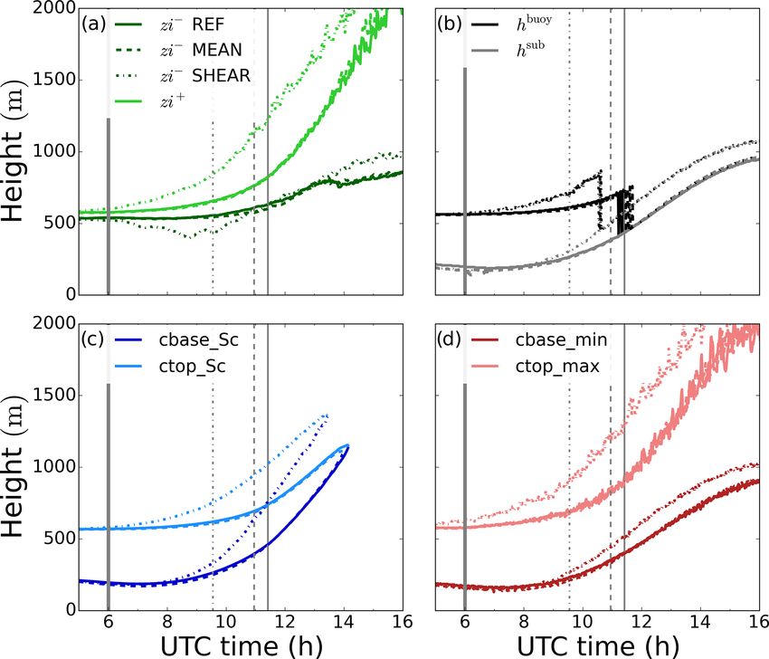
2736                            X. Pedruzo-Bagazgoitia et al.: The diurnal stratocumulus-to-cumulus transition over land

ing during the monsoon season between May and Septem-              the sea, surface fluxes are low and show little diurnal varia-
ber (van der Linden et al., 2015; Hill et al., 2018). Possible     tion. Evaporation from the sea provides the necessary mois-
future changes in highly sensitive Sc forcings in SWA, such        ture to maintain the Sc layer, which is well-mixed from top
as anthropogenic regional aerosol increase (Boucher et al.,        cloud down to the surface by the turbulence generated at
2013) or the global CO2 rise (Schneider et al., 2019), further     the cloud top by radiative cooling (Wood, 2012). Transitions
motivate a better understanding of the boundary layer cloud        from Sc to shallow cumulus have also been studied through
dynamics over land in SWA.                                         LES mostly in maritime conditions (Bretherton et al., 1999a;
   During the monsoon season, the intertropical convergence        Sandu and Stevens, 2011; de Roode et al., 2016). Such transi-
zone shifts northward till 15◦ N, facilitating the extension of    tions are typically investigated using a Lagrangian approach
the maritime air masses inland. The arrival of the cooler, but     in which the trajectory of an air mass is followed as it is ad-
not necessarily moister, mass of air more than a 100 km in-        vected from the subtropics towards the Equator. An increas-
land facilitates the onset of Sc clouds over land (Adler et al.,   ing sea surface temperature and decreasing subsidence are
2019; Babić et al., 2019; Dione et al., 2019). The fact that      usually imposed along the trajectory, leading to increasing
this mass of air is characterized by cloudless conditions when     latent heat fluxes and boundary layer height, respectively.
over the sea reveals the importance of the land and other lo-      The main mechanism for such transitions over the sea is
cal factors for the cloud formation and maintenance (Adler         the increase in buoyancy along the cloud layer by higher la-
et al., 2019; Babić et al., 2019; Lohou et al., 2019). Lohou      tent heat flux, leading to larger entrainment velocities aided
et al. (2019) extended the previous work and summarized            by the subsidence decrease, and the eventual dissipation of
the four phases leading from cloud formation to dissipation:       the Sc cloud layer. Over land, however, such transitions may
stable phase, jet phase, stratus phase and convective phase.       have different drivers, given their differently partitioned sur-
In addition, they described three observed scenarios for the       face fluxes as well as their larger magnitude and diurnal vari-
breakup and dissipation of the Sc deck throughout the day.         ability than over the sea. Ghonima et al. (2016) performed a
Such scenarios differed for the Sc coupling to surface and         thorough idealized LES study on Sc–Cu transitions both over
for the presence of convective clouds below the Sc.                land and over the sea. They based all their cases on vertical
   The high albedo of low-Sc clouds and their misrepresenta-       profiles of mid-latitude marine conditions and prescribed dif-
tion by most climate models lead to significant biases in the      ferent Bowen ratios to regulate the surface fluxes over land.
regional surface energy balance, especially if the evolution       They found that the Bowen ratio determines whether the sur-
and spatial structure of the cloud field is not correctly repre-   face fluxes lead to a thinning or thickening of the cloud layer.
sented (Hannak et al., 2017). More specifically, the mainte-       This was proved by a set of systematic experiments. Further-
nance, dissipation or transition to other cloud forms of the Sc    more, they provided a set of Bowen ratio-dependent feed-
cloud layer after sunrise have strong implications for the re-     backs highlighting the relevant role of the land: one feedback
gional energy balance (Knippertz et al., 2011; Hannak et al.,      loop where the increase in sensible heat flux would increase
2017; Lohou et al., 2019). These biases are less relevant dur-     entrainment, thinning the cloud layer, enhancing the net ra-
ing the night due to the absence of shortwave radiation, as        diation at the surface and further increasing the sensible heat
cloud-induced variations in the longwave radiation are 1 or-       flux. They provided two more feedbacks related to latent heat
der of magnitude smaller than those of shortwave radiation.        flux (LE): one in which its increase moistens and thickens the
To improve our understanding and to better quantify the ef-        cloud layer, decreasing net radiation and surface and, conse-
fects of Sc clouds over land in an observation-scarce region,      quently, LE; and another in which the LE increase enhances
the Dynamics-aerosol-chemistry-cloud interactions in West          entrainment, leading to cloud thinning and a further increase
Africa (DACCIWA) project deployed an extensive network             in LE. In contrast to mid-latitude marine conditions, atmo-
of observations during June and July in 2016 comprising            spheric conditions in near-equatorial SWA are characterized
three fully instrumented supersites (Knippertz et al., 2015;       by a moister and warmer atmosphere as well as stronger solar
Flamant et al., 2018; Kalthoff et al., 2018). The resultant        irradiation and, locally, larger evapotranspiration. These dif-
dataset with high spatio-temporal observations of the cloud        ferences pose the question of whether the mechanisms and
transition allows us to tackle two important questions. Firstly,   physical processes identified by Ghonima et al. (2016) re-
it allows us to understand the transition (Lohou et al., 2019)     main relevant for SWA.
and, using idealized numerical simulations, reproduce a char-         Our study thus aims at filling the knowledge gap on
acteristic stratocumulus-to-cumulus (Sc–Cu) transition with        turbulence-resolving numerical experiments of Sc–Cu tran-
typical conditions of SWA. Secondly, we aim at identifying         sitions taking place over land and, specifically, in subtropical
the physical processes and their complex interplay that leads      atmospheric conditions. We systematically focus on the fol-
to a breaking-up of the Sc deck.                                   lowing processes and the role played in the maintenance of
   Here, we extend the impacts of the land–atmosphere inter-       the Sc and its transition to cumulus clouds: radiation, entrain-
actions on the Sc–Cu transition and breakup. Previous stud-        ment and the land surface fluxes. Net longwave radiation is
ies have largely relied on high-resolution explicit modeling,      the source for cloud maintenance during the night through
e.g., large eddy simulation (LES), of marine Sc clouds. Over       cloud top cooling. As the day progresses, increasing short-

Atmos. Chem. Phys., 20, 2735–2754, 2020                                             www.atmos-chem-phys.net/20/2735/2020/
X. Pedruzo-Bagazgoitia et al.: The diurnal stratocumulus-to-cumulus transition over land                                     2737

wave radiation becomes a factor for dissipation. Entrainment      Sc–Cu transitions over the sea (van der Dussen et al., 2013;
is known to affect the cloud layer by drying and warming it,      de Roode et al., 2016). Here, we use the DALES 4.1 ver-
raising it and weakening the thermal inversion. The land sur-     sion. We describe below the relevant parameterizations for
face fluxes respond to variations in wind and radiation and       this study.
affect the transport of heat and moisture to the cloud layer
                                                                    – An interactive land surface model with a mechanistic
as well as the entrainment. In addition, we briefly study the
                                                                      representation of plant behavior. It regulates the sur-
evolution of metrics frequently used by parameterizations in
                                                                      face latent, and sensible heat fluxes, as well as the CO2
larger-scale models in the Sc–Cu transition.
                                                                      flux depending on environmental variables such as CO2
   Finally, during the DACCIWA campaign a recurrent low-
                                                                      concentration, atmospheric vapor pressure deficit, tem-
level jet along the cloud layer was observed (Adler et al.,
                                                                      perature, soil moisture and surface wind (Jacobs and
2019; Dione et al., 2019), raising an additional question re-
                                                                      de Bruin, 1997; van Heerwaarden et al., 2010; Vilà-
garding the effects of wind shear on Sc and its transition (Lo-
                                                                      Guerau de Arellano et al., 2015). It is upgraded with
hou et al., 2019). Previous work on modeled sheared Sc over
                                                                      a two big-leaf (sunlit and shaded leaves) scheme al-
the sea suggests that shear at the cloud top lowers the water
                                                                      lowing for different penetration rates of direct and dif-
content of Sc by enhancing the entrainment rate (Wang et al.,
                                                                      fuse radiation along the canopy (Pedruzo-Bagazgoitia
2008, 2012). Mechem et al. (2010) presented a land Sc case
                                                                      et al., 2017). The fact that surface fluxes are higher
and briefly studied the effects of shear. They similarly con-
                                                                      and more variable over land, responding to environmen-
cluded that in the presence of cloud top wind shear, entrain-
                                                                      tal variables and potentially altering the boundary layer
ment velocity increases, leading to a decrease in cloud liquid
                                                                      and cloud structure, explains the need for an interactive
water content. However, to the best of our knowledge, there is
                                                                      scheme such as the one presented here. Further details
no work studying the effects of wind shear on stratocumulus-
                                                                      on the settings of the land surface scheme are presented
to-cumulus transitions. Thus, we additionally perform some
                                                                      in Sect. 2.3.
sensitivity studies on the effect of wind and wind shear at the
cloud top on the Sc–Cu transition.                                  – The two-stream radiation scheme Rapid Radiative
   Our research seeks to answer these three research ques-            Transfer Model for use in GCMs (RRTMG; Iacono
tions:                                                                et al., 2008). It is used to provide longwave and di-
    – How is a stratocumulus-to-cumulus transition over land          rect and diffuse shortwave radiation at each grid box
      characterized? What is the relevance of the local pro-          depending on liquid water and other chemical com-
      cesses?                                                         pounds. This scheme allows us to represent the surface
                                                                      dynamic heterogeneities caused by cloud spatial inho-
    – How do the contributions of each physical process vary          mogeneities, as it provides a column-dependent net ra-
      with time during the maintenance, thinning and transi-          diation at the surface.
      tion of the cloud layer?
                                                                    – The microphysics scheme by Khairoutdinov and Kogan
    – How do these high-resolution simulations quantify met-          (2000), specifically designed for Sc clouds. It includes
      rics relevant for larger-scale models during the transi-        cloud-droplet sedimentation, found to be highly rele-
      tion?                                                           vant in the representation of Sc clouds (Ackerman et al.,
                                                                      2004; Bretherton et al., 2007; Dearden et al., 2018).
2     Methods                                                        The subgrid turbulence is parameterized using a tur-
                                                                  bulence kinetic energy (TKE) model following Deardorff
2.1    Dutch Atmospheric Large Eddy simulation                    (1980). Fifth- and second-order schemes are used to compute
                                                                  the advection over horizontal and vertical directions, respec-
To explicitly resolve the Sc–Cu transition we perform our         tively. The integration of the governing equations over time
numerical experiments using the Dutch Atmospheric Large           is carried out using a third-order Runge–Kutta scheme. For a
Eddy Simulation (DALES) (Heus et al., 2010; Ouwersloot            deeper insight in the mentioned numerical settings, the reader
et al., 2016). LES models explicitly resolve most of the          is referred to Heus et al. (2010). In particular, Eqs. (25), (43)
energy-containing turbulent motions in the boundary layer,        and (49).
including the stratocumulus and shallow cumulus cloud dy-
namics. Based on the initial work of Nieuwstadt and Brost         2.2   Observations
(1986), DALES is an LES model that has been used individ-
ually or within a model intercomparison for a broad range         We base our idealized study on observations taken during the
of cases, from clear-sky diurnal cycles (Pino et al., 2003)       field campaign of the DACCIWA project during the months
to boundary layers topped by stratocumulus (Blossey et al.,       of June and July 2016. We focus on the observations of
2013; van der Dussen et al., 2015) or cumulus (Siebesma           26 June 2016 at the Savè supersite. On this day a stratocumu-
et al., 2003; Vilà-Guerau de Arellano et al., 2014), including    lus deck was observed during the night and morning above

www.atmos-chem-phys.net/20/2735/2020/                                              Atmos. Chem. Phys., 20, 2735–2754, 2020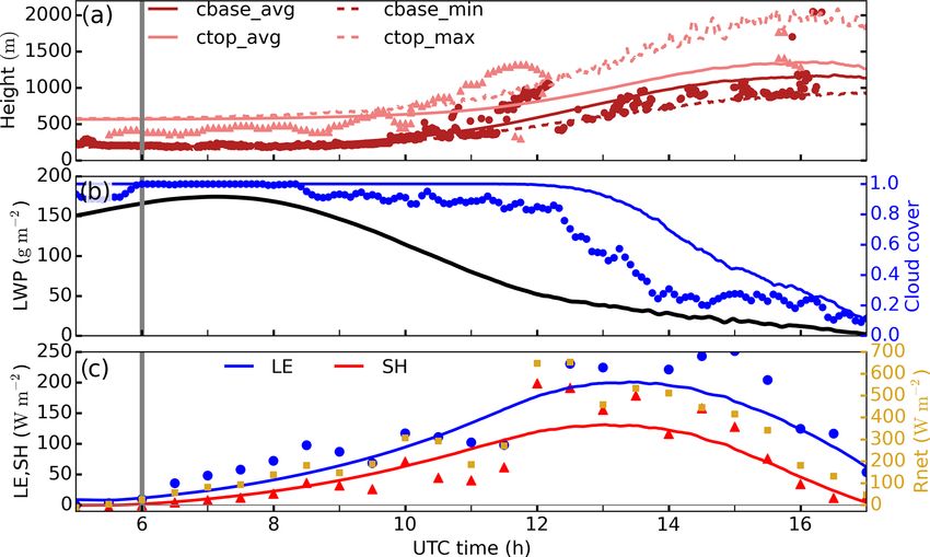
2738 X. Pedruzo-Bagazgoitia et al.: The diurnal stratocumulus-to-cumulus transition over land
Savè, followed by a cloud base rise and breakup during the
late morning and afternoon (Dione et al., 2019). We briefly
describe below the methods and observations used to inspire
our idealized study. For a fully detailed explanation of the ob-
servations and the dataset, the reader is referred to Kalthoff
et al. (2018) and Bessardon et al. (2020), respectively.
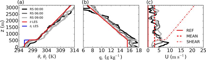
– Radiosondes were performed with the MODEM ra- Figure 1. Vertical profiles of potential temperature (a), total spe-
diosounding system. The temperature and relative hu- cific humidity (b) and wind (c) as observed through radioson-
midity of the air were measured with a 1 s temporal des (at 00:00, 06:00 and 09:00 UTC from black to light grey) on
resolution (' 4–5 m in vertical resolution). The wind 26 June 2016 and as prescribed in the idealized LES experiments
speed, direction and the pressure were determined based (red and blue). The three experiments REF, MEAN and SHEAR
on the radiosonde GPS coordinates (Derrien et al., differ only in the prescribed wind profiles.
2016).
– The cloud base height is measured by a continuously 2.3 Model settings and initial conditions
running ceilometer measuring backscatter profiles with
a 1 min resolution. Three cloud base heights are ob- Constrained by the surface and upper-atmospheric observa-
tained from the backscatter profiles using the manufac- tions, we design an academic case to be simulated through
turer algorithm. We select the lowest cloud base to en- LES. Our aim, by means of an idealized numerical ex-
sure that the detection reflects a cloud base and not, for periment, is to simulate a Sc–Cu transition, including the
example, a cloud edge. The data are available at Handw- Sc breakup, during typical atmospheric conditions in SWA
erker et al. (2016). rather than the reproduction of an exact day that occurred
during the DACCIWA measurement campaign. In particular,
– The cloud top height is measured by a dual-polarized
we study the Sc–Cu transition of a coupled case or Scenario
cloud radar, which allows us to distinguish between hy-
1 as described in Lohou et al. (2019).
drometeors and other targets. The cloud top height is es-
We design a 12 × 12 km2 wide and 3.2 km high domain,
timated from the 5 min averaged reflectivity profiles of
with a grid box size of 50 × 50 × 4 m3 resulting in 800 ver-
hydrometeors applying a threshold of −35 dBz (Bauer-
tical levels. Such high vertical resolution is required in order
Pfundstein and Goersdorf, 2007). Therefore, reflectivi-
to reduce the overestimation of mixing and entrainment typ-
ties larger than −35 dBz are considered clouds. The data
ical of coarser LES simulations with Sc (Bretherton et al.,
are available at Handwerker et al. (2016).
1999b; Stevens et al., 2005). Although at this vertical reso-
– The cloud cover is calculated as the percentage of cloud lution, processes such as evaporative cooling and cloud top
base height measurements below 1000 m (Adler et al., mixing might still be overestimated (Stevens et al., 2005;
2019; Zouzoua, 2020). The values are averaged over Mellado, 2017), a much finer resolution, or a direct numerical
19 d of the campaign to prevent too high a variability simulation approach, would not allow computationally for an
by single point observations at individual days. integrated simulation of both cloud top and ground surface.
As will be shown later, both interfaces play a critical role
– The surface fluxes and net radiation are obtained from in the development and transition studied here. We use pe-
an energy balance station deployed over a mix of grass riodic boundary conditions on the horizontal directions. We
and bushes. The 30 min sensible and latent heat fluxes start the experiment at 03:30 UTC to allow for 1 h of spin-up
are calculated from high-frequency (20 Hz sampling of the Sc layer and end the experiment at 18:30 UTC after
rate) measurements of wind speed and sonic temper- sunset.
ature obtained by ultrasonic anemometer and humid- The vegetation near and around the site consisted of het-
ity measurements which are based on the absorption of erogeneous patches containing shrubs, crops or taller trees
near-infrared radiation and obtained by a fast-response in very dense thickets with areas in the order of 50–100 m,
LI-COR sensor by applying eddy-correlation method a size too small to lead to the formation of secondary circu-
(Mauder et al., 2013). The data are available at Kohler lations (Patton et al., 2005). Unfortunately, no detailed mea-
et al. (2016). surements were taken on the vegetation types and properties
during the DACCIWA campaign. Thus, the case presented
– The two sets of turbulent kinetic energy measurements here shows spatially homogeneous soil and vegetation prop-
are calculated from the anemometer measurements of erties and is constrained taking into account the information
wind speed at 4 and 7.8 m by two energy balance sta- available on the surface fluxes. The land surface model al-
tions deployed over a mix of grass and bushes and over lows for spatially heterogeneous values of the surface fluxes
corn, respectively. depending on environmental conditions. This is known to be
Atmos. Chem. Phys., 20, 2735–2754, 2020 www.atmos-chem-phys.net/20/2735/2020/
X. Pedruzo-Bagazgoitia et al.: The diurnal stratocumulus-to-cumulus transition over land                                        2739

essential to realistically simulate clear (Patton et al., 2005)     an increase could be related to the previously questioned re-
and cloudy (Sikma and Vilà-Guerau de Arellano, 2019) con-           liability of radiosonde measurements as they exit the cloud
vective boundary layers. The terrain around the measuring           layer during their ascension (Lorenc et al., 1996; Mechem
site was relatively flat (Adler et al., 2019), allowing us to as-   et al., 2010; Babić et al., 2019). Situations without a dry jump
sume a topography-free domain. Thus, assuming a flat and            above the Sc cloud top have been previously reported over
homogeneous surface simplifies our study and permits us to          land (Mechem et al., 2010) and are more typical of arctic
focus on the local effects that can be more easily general-         climates (Morrison et al., 2012).
ized to similar situations in SWA. Meanwhile, the dynamic              The observations demonstrate that the idealized experi-
heterogeneities created guarantee a sufficiently realistic rep-     ment’s initial conditions lie within typical meteorological
resentation of the boundary layer during the day.                   conditions in SWA. The initial idealized profiles prescribe a
   We prescribe a subsidence profile, following Bellon and          well-mixed layer up to 570 m with liquid water potential tem-
                                                        −z
Stevens (2012), of the shape wsubs (z) = −w0 (1 − e zw ), with      perature θl = 296 K and specific humidity qt = 15.5 g kg−1 .
w0 = 5.3 mm s−1 and zw = 300 m. Such a profile translates           Such thermodynamic conditions result in a domain-covering
into wsubs = −4.51 mm s−1 at the initial cloud top height           cloud layer from 226 to 570 m high, topped by a jump of
of 570 m. Our choice for the subsidence profile was such            4.5 K in temperature, but without a jump in specific humid-
that it would keep a nearly constant cloud top height dur-          ity. Above 570 m the potential temperature and total moisture
ing the night, and it is justified given the uncertainty and        idealized profiles exhibit constant slopes of 4.67 K km−1 and
high temporal variability in subsidence profiles, as well as        3.29 g kg−1 km−1 , respectively. Given the spread in vertical
its large spread among regional simulations carried out with        profiles by radiosondes, we performed additional simulations
the Consortium for Small-Scale Modeling (COSMO) within              exploring variations in the profiles of 0.5 K and 0.5 g kg−1 .
the DACCIWA project or ERA-interim. For simplicity we as-           Results showed a very similar development of the Sc–Cu
sume the subsidence profile to be constant during the entire        transition.
simulation. To limit the complexity of our idealized experi-           Our reference experiment REF prescribes no wind at any
ments and focus on the interaction of the surface and bound-        heights. To study the effect of wind and wind shear, we per-
ary layer processes, we prescribe no advection of heat or           form two additional numerical experiments – MEAN and
moisture at any height. Adler et al. (2019) and Babić et al.       SHEAR – where we account for different idealized wind ef-
(2019) found cold air advection necessary for the formation         fects. This sensitivity analysis is motivated by the recurrent
of the cloud layer. Yet its relevance decreased as sunrise ap-      winds with the shape of low-level jet, such as those in Fig. 1c,
proached, thus justifying our assumption.                           that were frequently observed during the DACCIWA cam-
   For all the experiments we calculate the vertical profiles       paign (Kalthoff et al., 2018; Adler et al., 2019; Dione et al.,
of the radiative fluxes every minute. In doing so, we quan-         2019). Failed attempts to maintain a low-level jet-like wind
tify how radiative fluxes are perturbed by the liquid water         profile together with the Sc cloud layer in preliminary exper-
related to cloud dynamics and how they interact with the sur-       iments suggest that the jet-like wind is the result of large-
face. This is done to account for fast fluctuations of net ra-      scale dynamics and, thus, beyond the scope of the present
diation at the cloud top and surface. The latter is relevant        study on local factors. The large-scale origin of the low-level
given its potential to alter surface fluxes and, thus, the evolu-   wind is also supported by more detailed observational analy-
tion of the boundary layer and clouds (Vilà-Guerau de Arel-         sis (Babić et al., 2019; Adler et al., 2019; Dione et al., 2019).
lano et al., 2014; Gronemeier et al., 2016; Sikma and Vilà-         Following our idealized approach, the initial wind speed and
Guerau de Arellano, 2019). Based on aircraft observations           wind direction are inspired by the observations and adapted
during the DACCIWA campaign (Taylor et al., 2019), the              to better study how these effects influence the Sc–Cu transi-
cloud droplet number concentration is set to 300 cm−3 and           tion. In this case, the mean wind and the shear at the cloud top
remains constant throughout the experiment. No radiative ef-        are considered. We prescribe a constant horizontal wind of
fects of aerosols are taken into account here.                      3 m s−1 along the whole vertical profile in MEAN based on
   We show in Fig. 1 the vertical profiles obtained                 above-cloud-layer radiosonde observations (Fig. 1c). Consis-
through three radiosondes during the night and morning of           tent with our idealized setting, we assume the wind to blow
26 June 2016. The radiosonde at 06:00 UTC, the closest              only along the x direction and without prescribed directional
to our initialization time, shows a strong increase in po-          shifts with height. In SHEAR we add a jump of 5 m s−1 to
tential temperature of about 3 K at 570 m high. Above, all          the mean 3 m s−1 at the cloud top to represent a wind shear
radiosondes show similar temperature lapse rates of about           of a similar magnitude as the observed low-level jet. The
4.6 K km−1 . Subtropical marine Sc clouds are frequently            values prescribed here for the simplified effects of the low-
capped by much drier air above the cloud top (Duynkerke             level jet are representative not only of the day studied here
et al., 2004; Wood, 2012). Yet none of the radiosonde profiles      but also of the whole measurement campaign (Dione et al.,
show any strong jump in moisture above 570 m. If anything,          2019). The free-troposphere wind shows a constant increase
they show a humidity increase above the cloud layer. Such           of 5 m s−1 km−1 in SHEAR. Our aim here is to maintain
                                                                    a shear contribution as the cloud layer rises. We prescribe

www.atmos-chem-phys.net/20/2735/2020/                                                Atmos. Chem. Phys., 20, 2735–2754, 2020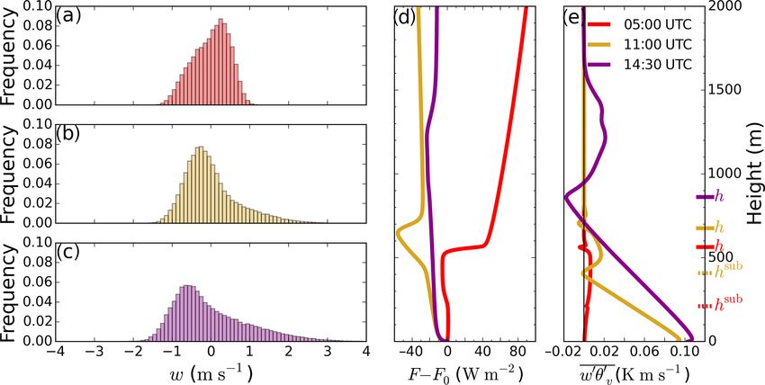
2740                            X. Pedruzo-Bagazgoitia et al.: The diurnal stratocumulus-to-cumulus transition over land

geostrophic winds identical to the initial wind profiles, as the   of the convective phase, defined by Lohou et al. (2019) as
goal is to observe the impact of wind on the transition and        the time when the sensible heat flux SH > 10 W m−2 , takes
not vice versa. In summary, differences between MEAN and           place between 07:00 and 07:30 UTC according to observa-
REF serve in identifying the role played by a mean wind,           tions and at 06:55 UTC in REF. The breakup in the cloud
which will mainly enhance the surface fluxes. MEAN and             layer, defined as the time when cloud cover (cc) is below
SHEAR differences show the impact of the local shear at the        1, takes place at around 11:30 UTC in the LES experiment
cloud top.                                                         and coincides with the observed sharp increase in surface
   To determine the dependency of the results on the Galilean      fluxes of about 150 W m−2 , i.e., a 3-fold increase compared
transformation, we performed two extra simulations. We re-         to before-breakup values. This sudden change coincides with
produced the MEAN experiment with an additional grid               the sharp increase in net radiation due to cloud breakup (see
translation of 3 m s−1 identical to the prescribed mean wind,      Fig. 2c) and reveals that surface fluxes are radiation-driven at
and the SHEAR experiment with a grid translation of                this stage. The good agreement in the surface flux partition-
6 m s−1 . These additional experiments yielded very similar        ing as modeled and observed justifies the use of a land sur-
results to the original ones and confirmed the independence        face model sensitive to several environmental variables at the
of our numerical experiments on this condition. Therefore,         surface (see Sect. 2.1). After 11:30 UTC observations show
for the sake of simplicity none of the simulations shown here      large variability in measured cloud base heights (Fig. 2a),
have Galilean transformation prescribed.                           suggesting either the presence of shallow clouds below the
                                                                   Sc cloud layer or the breakup of the Sc layer (Lohou et al.,
                                                                   2019). Therefore, the jump in cloud base height from about
3     Results                                                      1000 to 500 m is due to either the appearance of the first
                                                                   shallow cumulus at 500 m after the stratocumulus cloud base
3.1    Evolution of the transition                                 rises up to 1000 m or to the breakup of the stratocumulus
                                                                   deck leading to different observed cloud base heights. About
Figure 2 shows the diurnal evolution of cloud height, cover
                                                                   90 min after cloud breakup, cc decreases quasi-linearly until
and liquid water path (LWP) and their connection with sur-
                                                                   the end of the simulation. The same pattern for cloud cover is
face turbulent fluxes in the REF simulation. It also includes
                                                                   shown by observations, although 1 h earlier. Note, however,
the observations corresponding to the day by which our case
                                                                   that the observations of cc are averaged over 19 d selected
is inspired. At Fig. 2a both cloud top and base remain ap-
                                                                   due to cloud onset happening before 04:00 UTC (Zouzoua,
proximately constant for the first hours. The LWP values are
                                                                   2020). The variability between the days considered in the av-
at the high end of domain-average LWP for marine stratocu-
                                                                   erage also explains the cc values below 1 before 06:00 and
mulus cloud (Wood, 2012) and coincide with observed ones
                                                                   after 08:30 UTC.
during the DACCIWA campaign (Babić et al., 2019; Kalthoff
et al., 2018). The initially constant cloud top height coincides
with the boundary layer height. As a result, the boundary          3.2   Transition on turbulence and radiation
layer height evolution can be expressed using mixed layer
theory by the relation that equates the entrainment veloc-         The turbulent spatial structure explaining this transition
ity and the subsidence. Assuming horizontally homogeneous          from typical nocturnal stratocumulus to convective clouds is
conditions, it reads (Lilly, 1968)                                 shown in Fig. 3 through the buoyancy flux and temperature
                                                                   profiles. The initial stages of the LES experiment (Fig. 3a,
∂h                                                                 b, c) present a well-mixed and fully coupled layer from the
   = we + wsubs (h) ' 0                                     (1)
∂t                                                                 surface to the cloud top. This layer is limited by a strong
                                                                   jump in liquid water potential temperature θl of about 4 K at
with h the boundary layer height defined as the height of          05:00 UTC (Fig. 3a) at around 550 m and a very thin inver-
minimum buoyancy flux, we the entrainment velocity and             sion layer. We quantify this layer through its lower and upper
wsubs (h) the subsidence, depending on height as described         limits zi − and zi + , respectively. These heights are defined,
in Sect. 2.3, at h. For this experiment and before sunrise         following van der Dussen et al. (2016), as the heights above
we ' −wsubs (h) = 0.45 cm s−1 , which is in the same order
                                                                   and below, respectively, the maximum in slab-averaged θl0 2
of magnitude as previously reported nocturnal marine Sc                   max                        max
cases (Stevens et al., 2003). Between 2 to 3 h after sun-          and θl0 2 , at which 5 % of θl0 2    is reached. The thresh-
rise (06:00 UTC) the cloud layer begins to rise and subse-         olds defining zi − and zi + are set to be constant over the
quently decreases its liquid water content (Fig. 2b), allowing     whole simulation for the sake of consistency and easier com-
more radiation to reach the surface and enhancing the sur-         parison with previous studies. In Fig. 3b, the liquid water
face fluxes (see Rnet , LE and SH increase between 06:00 and       mixing ratio ql shows a linear increase with height within
10:00 UTC in Fig. 2c). During this time the domain-average         the cloud layer typical of well-mixed stratocumulus clouds
cloud base cbase_avg follows the observed cloud base and           (Duynkerke et al., 1995; Wood, 2012). After some hours
so do the surface fluxes with the observed ones. The onset         the boundary layer evolves into a well-mixed subcloud layer

Atmos. Chem. Phys., 20, 2735–2754, 2020                                             www.atmos-chem-phys.net/20/2735/2020/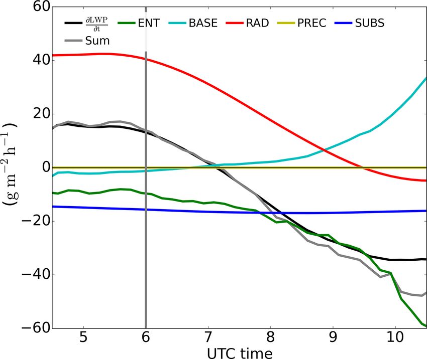
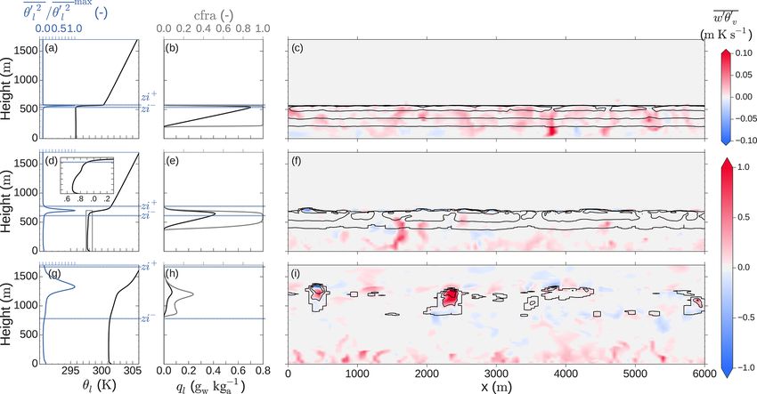
X. Pedruzo-Bagazgoitia et al.: The diurnal stratocumulus-to-cumulus transition over land                                                   2741

Figure 2. Time series of the domain-average cloud base (cbase_avg as solid dark red line) and cloud top (ctop_avg as solid light red line),
maximum cloud top (ctop_max in dashed light red line) and minimum cloud base (cbase_min in dashed dark red line) (a), liquid water path
and cloud cover (b), and latent and sensible heat fluxes as well as net radiation (c) in REF. Observed cloud base and cloud top heights on
26 June are represented by dark red circles and light red triangles, respectively, in (a). Observed cloud cover, averaged over 19 campaign
days is shown in blue circles in (b). Observed latent and sensible heat fluxes are shown by blue circles and red triangles, respectively, and net
radiation in yellow squares in (c). The vertical grey lines indicate the sunrise time.

Figure 3. On the left (a, d, g), slab-averaged vertical profile of liquid potential temperature θl (black) and θl0 2 normalized over its maximum
value (blue). The inversion layer upper zi + and lower zi − limits are indicated by dashed blue horizontal lines. In the center (b, e, h) slab-
averaged vertical profiles of liquid water mixing ratio ql (black) and horizontal cloud fraction cfra (grey). On the right (c, f, i), horizontal
cross section of buoyancy flux w 0 θv0 (red (blue) indicating upwards (downwards) movement of buoyantly positive (negative) air) and cloud
liquid water (in black contour lines every 0.3 gw kg−1a ). Panels (a), (b) and (c) correspond to 05:00 UTC, (d), (e) and (f) to 11:00 UTC, and
(g), (h) and (i) to 14:30 UTC. The inset in (d) is an expanded version of the rectangle in the same panel.

www.atmos-chem-phys.net/20/2735/2020/                                                         Atmos. Chem. Phys., 20, 2735–2754, 2020
2742                              X. Pedruzo-Bagazgoitia et al.: The diurnal stratocumulus-to-cumulus transition over land

Figure 4. On the left, frequency distribution of vertical velocities at h2 at 05:00 UTC (a), 11:00 UTC (b) and 14:30 UTC (c). In the center (d),
vertical profile of slab net radiative flux normalized over the surface value at 05:00 UTC (red), 11:00 UTC (dark yellow) and 14:30 UTC
(purple). On the right (e) and following the same color code, slab-averaged buoyancy flux w0 θv0 . The subcloud layer height hsub and the
boundary layer height h are shown for each time at the right vertical axis in (e). At 14:30 UTC both heights coincide.

with a conditionally unstable cloud layer aloft at 14:30 UTC              diation through the cloud layer down to the surface is key
and a very broad inversion layer. Such evolution of the inver-            in regulating both phenomena. The warming of the cloud
sion layer enables us to interpret the typically conditionally            layer leads to a decoupling of the cloud and subcloud lay-
unstable region of the cloudy layer in convective conditions              ers. This is already visible at 11:00 UTC with a temperature
as an expanded analogue of the very sharp inversion layer                 difference between layers of about 0.2 K at 400 m high (see
near the top of Sc clouds. Note that this layer includes the              inset in Fig. 3d).
sharper inversion layer common in cumulus-topped bound-                      By resolving interactively the radiation transfer along the
ary layers and present in Fig. 3g, h, i between 1200 and                  cloud layer and the surface response, we gain insight into
1300 m. Thus, to correctly represent the transition studied               the dynamical transition, as shown in Fig. 4. There, we ob-
here it is necessary to treat the evolution as a transition where         serve how the vertical velocity distribution in the middle of
the inversion layer expands as the boundary layer grows. A                the boundary layer starts from a situation with limited ex-
more detailed evolution of the inversion layer is given in                treme velocities (between −1.3 and 1 m s−1 ) and a negative
Fig. 5. Furthermore, the cloud fraction in the lower part of                                                                              w0 3
                                                                          skewness of Sw = −0.3 at 05:00 UTC, where Sw =                     3    .
the cloud layer at 14:30 UTC resembles that of shallow cu-                                                                               w0 2 2
mulus clouds (Siebesma et al., 2003). In this case, however,              This value for Sw lies within the limits of typical marine
a second peak in cloud fraction and larger ql reveals the pres-           Sc clouds (Ghate et al., 2014). It then evolves into a pro-
ence of more clouds at around 1200–1300 m. These clouds                   totypical convective boundary layer (CBL) skewed distribu-
are the remnants of the stratocumulus higher part.                        tion with a larger spread of vertical velocities at 11:00 UTC
   In the absence of mechanical production of turbulence,                 (between −1.5 and 2.7 m s−1 ) and Sw = 1.2 at half of the
buoyancy is the only driving mechanism for turbulence.                    boundary layer height, these skewness values being typical
Figure 3c, f and i quantify the shift of buoyancy-driven                  of dry convective boundary layers (Lenschow et al., 2012)
turbulence generation from cloud top radiative cooling at                 or situations with cumulus coupled to Sc clouds (de Roode
05:00 UTC to surface warming at 14:30 UTC. Note the                       and Duynkerke, 1996). Similar values for Sw are found at
change in scale by a factor of 10 in w0 θv0 between Fig. 3c               14:30 UTC, with minimum and maximum vertical veloci-
and i. Such a difference in magnitude shows that the surface-             ties between −1.8 and 3.5 m s−1 , respectively. The transition
driven turbulence after sunrise becomes stronger, by about                from stratocumulus to prototypical convective conditions is
10 times, than the one created by cloud top cooling. In fact,             reinforced by the evolution of the radiative profiles. Figure 4d
the cloud top cooling contribution to the buoyancy flux is in             shows an initial net radiative divergence at the cloud top
part diminished by a compensating condensational warming                  of 43 W m−2 . The related cooling drives the mixed layer at
within the cloud layer. At 11:00 UTC there is a critical mo-              05:00 UTC. At this time the radiative cooling is stronger than
ment in the transition: the cloud layer remains rather homo-              the warming by entrainment as the mixed layer cools at a rate
geneous, but the mixed layer is now simultaneously driven                 of about 0.1 K h−1 before sunrise (not shown). By 11:00 UTC
both by surface warming and cloud top cooling. As will be                 there is a net radiative warming along the cloud layer (be-
shown later (Figs. 4 and 6), the penetration of shortwave ra-             tween 400 and 650 m high; see Fig. 3) due to the absorption

Atmos. Chem. Phys., 20, 2735–2754, 2020                                                      www.atmos-chem-phys.net/20/2735/2020/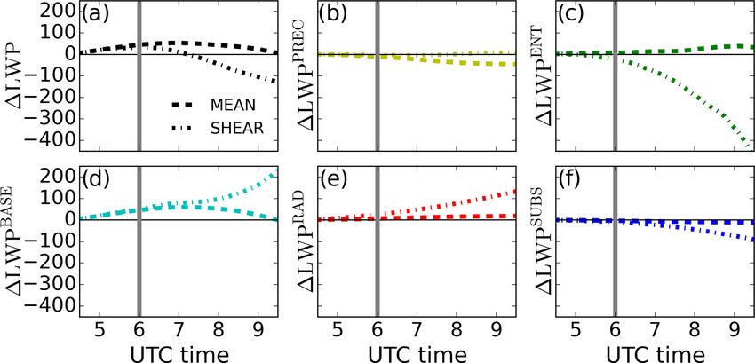
X. Pedruzo-Bagazgoitia et al.: The diurnal stratocumulus-to-cumulus transition over land                                          2743

of shortwave radiation within the cloud layer. Shortwave ra-
diation locally warms up the lower two thirds of the cloud
layer to 1.1 K h−1 due to the 44 W m−2 of absorbed short-
wave radiation along its travel through the cloud layer (not
shown). The high cloud droplet number, 300 cm−3 , is likely
to influence such net warming positively.
   This net radiative warming along the cloud layer re-
inforces the warming driven by entrainment of free-
tropospheric air. The combination of both processes is crit-
ical for the decoupling of the cloud and subcloud layers. As
will be shown later (Fig. 6), it also plays a role in the thinning
of the Sc and the reduction in turbulence generation at the
cloud top. Figure 4e shows the profile of the buoyancy flux,
closely linked to the role of radiation. The averaged buoy-
ancy flux shows a similar transition starting from prototyp-
ical nocturnal Sc clouds at 05:00 UTC, with positive buoy-
                                                                     Figure 5. Time series of inversion layer top zi + (light green) and
ancy along the whole layer up to 550 m and a local minimum           bottom zi − (dark green) heights, boundary layer height h (black)
at the cloud base due to latent heat release (Bretherton and         and subcloud buoyancy minimum height hsub (grey), stratocumu-
Wyant, 1997; Wood, 2012). We define the height of such a             lus cloud base cbase_Sc (dark blue) and top ctop_Sc (light blue)
minimum as the subcloud layer height hsub . The definition of        heights, and minimum cloud base cbase_min (dark red) and max-
hsub is necessary to better quantify the decoupling of the stra-     imum cloud top ctop_ max (light red) heights. Sunrise time and
tocumulus layer from the surface, as will be shown in Fig. 10.       cloud breakup time are indicated by the thick and thin grey lines,
At the cloud top, Fig. 4e presents an absolute minimum at the        respectively.
boundary layer height h at 05:00 UTC. The buoyancy flux
profile at 11:00 UTC shows the decoupling of the cloud layer
                                                                     on observations. The cloud and subcloud layer dynamics di-
from the surface by the enhancement of the local minimum
                                                                     vert from coupled Sc conditions, i.e., a well-mixed layer from
at hsub at 400 m. This nearly negative value in the vicinity
                                                                     the surface to the cloud top, several hours before, as was
of the cloud base has already been described as an indica-
                                                                     shown in Figs. 3 and 4. Between 11:00 and 11:30 UTC, i.e.,
tion of decoupling and hampered transport of moisture (and
                                                                     before the cloud breakup, h shifts from the cloud top to the
heat, in our case) from the surface to the cloud layer (Turton
                                                                     subcloud layer top represented by hsub . The evolution of the
and Nicholls, 1987; Stevens, 2000; Lewellen and Lewellen,
                                                                     inversion layer, indicated by zi + and zi − , reveals a broad-
2002). This will be further explored in Fig. 10. The buoy-
                                                                     ening of the inversion layer from a very thin layer (∼ 50 m)
ancy profile evolves at 14:30 UTC to a profile common in
                                                                     across the cloud top during the first few hours to a region
cumulus-topped convective boundary layers (Siebesma et al.,
                                                                     thicker than 1 km in the afternoon due to the cumulus clouds.
2003) or decoupled Sc cloud layers (Wood, 2012). It shows a
linearly decreasing w0 θv0 up to the cloud base and buoyantly        3.3    LWP budget before and during the transition
active convective clouds above 950 m. Note that under such
conditions the boundary layer height and the subcloud top            After observing the transition in cloud characteristics and
height coincide and hsub = h.                                        buoyancy regime, a question immediately arises: what is the
   We show in the time series in Fig. 5 the evolution of the         relative contribution of the main physical processes driving
variables that better reflect the dynamics of the Sc–Cu tran-        this transition? To this end and relating to Fig. 2b, LWP is
sition: we show the inversion layer upper and lower limits           calculated and used as the metric to describe the state of the
zi + and zi − , respectively, the subcloud top height hsub and       transition and calculate the budget derived by van der Dussen
boundary layer height h shown in Fig. 4, and the maximum             et al. (2014). The budget reads
cloud top and minimum cloud base heights as in Fig. 2, and
we additionally calculate the Sc cloud base cbase_Sc and             ∂LWP
                                                                          = BASE + ENT + PREC + RAD + SUBS,                         (2)
cloud top ctop_Sc. These are defined as the height of the              ∂t
lowest and highest vertical level, respectively, with a slab-        with
averaged cloud fraction higher than 40 %. After 10:00 UTC                                b             b
the Sc cloud base rises faster than the minimum cloud base.          BASE = ρη (w0 qt0 − 5γ w 0 θl0 ),
This is analogous to the slower rise of the Sc cloud top com-         ENT = ρwe (η1qt − 5γ η1θl − D0ql ),
pared to the maximum cloud top. Due to a faster rise of the
                                                                     PREC = −ρδP ,
Sc cloud base than the Sc cloud top, there is a thinning of the
Sc layer eventually dissipating at 14:00 UTC. Lohou et al.            RAD = ρηγ δFrad ,
(2019) observed a similar cloud thinning pattern based solely        SUBS = −ρD0ql ws (h),                                          (3)

www.atmos-chem-phys.net/20/2735/2020/                                                  Atmos. Chem. Phys., 20, 2735–2754, 2020
2744 X. Pedruzo-Bagazgoitia et al.: The diurnal stratocumulus-to-cumulus transition over land
15 %, driven solely by the longwave cooling at the cloud top
(RAD term). During the entire experiment SUBS remains al-
most constant given the small variation in subsidence with
height, showing a negative tendency of around 16 g m−2 h−1 .
The negative tendency by entrainment (ENT) is to a large
extent initially due to the entrainment of warm air (second
term in ENT in Eq. 3) since, as shown in Fig. 1, the free-
tropospheric air has a similar moisture content to the cloudy
air. The thinning tendency of precipitation is small, account-
ing for up to 4 g m−2 h−1 when the cloud layer is thickest.
The small contribution of PREC despite large LWP is ex-
plained by the microphysical characteristics of the region.
The large cloud condensation nuclei (CCN) concentrations
typical for SWA (300 cm−3 in our study) prevent any large
effects of precipitation even in Sc with high liquid water con-
Figure 6. Time series of budget terms as defined in Eqs. (2) and (3) tent. The effect by cloud base fluxes before sunrise is of a
with colors representing the terms as displayed in the legend, and similar magnitude: the turbulent transport of warm air (sec-
the sum grey line being the sum of all the terms on the right-hand ond term of BASE in Eq. 3) dominates over its moistening
side of Eq. (2). The vertical grey line indicates sunrise time. effect (first term of BASE in Eq. 3) at this time. Yet the neg-
ative net effect by BASE in the LWP tendency is about 10
orders of magnitude smaller than that of RAD.
with BASE representing the effect of turbulent fluxes at the After sunrise the warming effect of shortwave radiation in-
cloud base, ENT that of entrainment, PREC the effect of pre- creasingly offsets the longwave cooling at the cloud top. This
cipitation, RAD that of radiation, and SUBS the one due to leads to a decreasing contribution of RAD to the thickening
subsidence. 1qt and 1θl are the jumps across the inversion of the cloud layer. Due to this factor, the sign of the LWP ten-
layer for total water mixing ratio and liquid water potential dency changes at around 07:15 UTC. This is the time when
temperature, respectively, defined as in van der Dussen et al. the thinning leading to the eventual cloud breakup starts. Cor-
(2016): 1θl = θl (zi + )−θl (zi − ) and 1qt = qt (zi + )−qt (zi − ). related to the shortwave radiation increase after sunrise, the
δP and δFrad represent the difference in precipitation and net surface-driven growth of the boundary layer leads to larger
radiation, respectively, between the top of the inversion layer entrainment rates, thus increasing the warming of the cloud
zi + , assumed to be the same as Sc cloud top height in van der layer through the free-tropospheric engulfed air. An addi-
Dussen et al. (2016) and the Sc cloud base (van der Dussen tional factor to the already mentioned warming explains the
et al., 2016). The rest of the variables in Eq. (3) are listed in fast shift to more negative tendencies for the ENT term af-
Appendix A. ter 07:00 UTC: the increased drying through entrainment.
In short, this budget enables us to decompose the thin- This drying increases due to two factors enhancing 1qt , from
ning or thickening of the cloud layer, quantified by a LWP −0.27 g kg−1 at 07:00 UTC to −1 g kg−1 at 10:00 UTC: the
tendency, and relate each contribution to the physical pro- moisture input in the boundary layer by the surface and the
cesses governing the stratocumulus clouds. To derive such growth of the boundary layer itself across a drier free tropo-
a budget van der Dussen et al. (2014) assumed the cloud sphere. This larger moisture jump enhances the impact of en-
layer to be horizontally homogeneous and vertically well- trainment by (a) drying the cloud layer and (b) enhancing the
mixed, implying a linear increase in the liquid water with entrainment velocity as the difference in buoyancy between
height within the cloud layer following an adiabatic liquid the cloud and free troposphere decreases. By the end of this
water profile. The first hours of the simulation perfectly fit period, at 10:00 UTC, the positive contribution to LWP of
those conditions. However, after some hours the horizontal cloud base fluxes (BASE) rises to up to 30 g m−2 h−1 . This
heterogeneities created in the Sc layer and the formation of is explained by the increase in surface fluxes (Fig. 2c) and
convective clouds below (see Fig. 5) do not allow these as- surface buoyancy (Fig. 4e) as the available net radiation at
sumptions to hold any longer. Furthermore, the assumption the surface grows. These changes lead to a larger contribu-
of one well-mixed cloud layer breaks after 10:00 UTC due to b
tion of the moistening w 0 qt0 term to BASE in Eq. (3), while
the warming by radiation and entrainment (Fig. 4). The dis- b
tance between zi + and ctop_Sc, assumed to be negligible by the warming term including w0 θl0 remains less variable for
van der Dussen et al. (2014), increases with time up to 50 m the first hours. Note that although the moisture flux increase
at 10:00 UTC. For this reason we focus our analysis on the at the cloud base implies a growth of LWP in the budget,
first stage of the transition until 10:00 UTC. such moisture growth may eventually contribute to the dissi-
Before sunrise we observe in a net thickening of the cloud pation of the cloud layer: increased surface moisture flux at
layer Fig. 6 by almost 20 g m−2 h−1 , i.e., a growth of about the surface and consequently, at the cloud base, relates to en-
Atmos. Chem. Phys., 20, 2735–2754, 2020 www.atmos-chem-phys.net/20/2735/2020/X. Pedruzo-Bagazgoitia et al.: The diurnal stratocumulus-to-cumulus transition over land 2745
hanced buoyancy through latent heat release and larger turbu-
lence within the cloud layer, known to increase entrainment
(Ghonima et al., 2016; Kazil et al., 2016). Such accelerated
entrainment leads to the warming of the upper cloud and thus
counteracts the mixing of the cloud layer necessary for the
maintenance of the Sc.
Comparing the contributions before sunrise in our case to
those of the first night in van der Dussen et al. (2016), we
find a RAD term almost 30 % lower in our case. Given the
similar LWP and θl jump above the cloud top, we attribute
the significant difference to the lack of a moisture jump here
and thus, weaker cloud top radiative cooling. The BASE term Figure 7. Time series of accumulated differences between MEAN
and REF (dashed) and between SHEAR and REF (dotted–dashed)
reached values of about 60 g m−2 h−1 in van der Dussen et al.
for each term defined in Eq. (2) and calculated following Eq. (4).
(2016), while we found very little contribution of such a term
during the morning due to the compensation of moistening
and warming effect of turbulent fluxes. This large difference fect the evolution of the cloud transition described in previ-
compared to a marine case shows the relevance of the land ous sections. First, in Fig. 7 we show the relative differences
surface, as the moistening is limited here and counteracted by between the terms defined in Eq. (3) as part of the LWP bud-
a larger warming through turbulent fluxes at the cloud base get. Following van der Dussen et al. (2016), we show the
compared to a marine case. The nighttime ENT term is in our accumulated difference, starting at 04:30 UTC, of the LWP
case about 2 to 3 times smaller than in van der Dussen et al. tendency due to each term between MEAN or SHEAR and
(2016), explained by larger turbulence created by a stronger the reference simulation REF. Taking the precipitation con-
RAD in their study. All in all, the total tendency ∂LWP ∂t is tribution PREC as an example, we calculate
of the same order of magnitude for both cases, although the
drivers remain quite different. The increasing negative contri- Zt
PREC
bution to the LWP budget by entrainment at daytime is con- 1LWP (t) = PREC(t 0 ) − PRECREF (t)0 dt 0 (4)
sistent with the Sc-over-land case by Ghonima et al. (2016).
04:30 UTC
We find our case to fall between their cases with fixed Bowen
ratios of Bo = 0.1 and Bo = 1, as we observe nearly Bo = 0 and similarly for all the other terms present in Eq. (2).
during the night growing up to 0.6 during the day in the cur- The presence of a light mean wind (3 m s−1 ) in the entire
rent case, similar to the measured conditions (Fig. 2c). This domain only has minor effects on the first part of the tran-
indicates the advantage of having a land surface model cor- sition: Fig. 7 shows a slightly larger LWP for the MEAN
rectly partitioning the available net energy into surface and experiment compared to REF. The larger LWP is driven
latent heat fluxes. In our case, the BASE term behaves similar by the increased contribution of the turbulent fluxes at the
to their Bo = 0.1 case as it also shows a positive contribution cloud base (BASE) and particularly the contribution of the
to cloud thickening or LWP increase. moisture flux. For both MEAN and SHEAR experiments,
BASE shows a thickening contribution already before sun-
3.4 Effect of wind and wind shear in the transition rise, whereas it was a net thinning contribution in the REF
experiment. The change in BASE is explained as follows:
3.4.1 Nighttime effects wind enhances latent heat flux as well as turbulent genera-
tion near the surface, favoring the transport of moisture to
We showed that the transition from stratocumulus to cu- the cloud layer. The enhanced turbulence generation near the
mulus over land for typical SWA conditions can take place surface due to the wind, both in MEAN and SHEAR, is vis-
under windless conditions. Given the recurrent presence of ible in the lower part of Fig. 8a. We show there the contri-
wind and low-level jet in the morning during the observa- butions by the buoyancy and shear terms, B and S, respec-
tional campaign, it is interesting to further investigate the ef- tively, to the TKE tendency budget and the good agreement
fects that wind has on the transition. Thus, we extend the regarding surface TKE between our experiments and the ob-
previous results considering the further effects that mean servations. Enhanced LWP in nighttime Sc by the presence
wind (MEAN) and additional wind shear at the cloud top of wind was also found by Kazil et al. (2016) and attributed
(SHEAR) have on the transition described. In Table 1, we to enhanced buoyancy production of TKE due to latent heat
include the timing and magnitude of the reference metrics release in cloud updrafts. Such findings coincide with the en-
for each experiment. Under cloudless conditions, the effect hanced buoyancy term B for MEAN in Fig. 8a. Precipitation,
of shear at the surface as well as at the boundary layer top acting as a negative feedback on LWP, attenuates the effect
acts as a local source of TKE (Conzemius and Fedorovich, by BASE in the total tendency of LWP. The remaining terms
2006). In our case, such modifications in turbulence may af- show little variation between REF and MEAN.
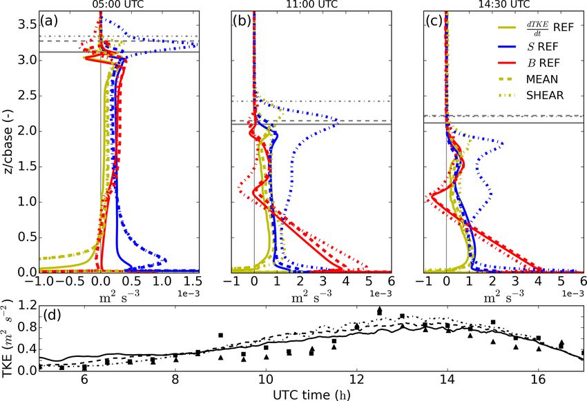
www.atmos-chem-phys.net/20/2735/2020/ Atmos. Chem. Phys., 20, 2735–2754, 20202746 X. Pedruzo-Bagazgoitia et al.: The diurnal stratocumulus-to-cumulus transition over land Figure 8. Slab-averaged vertical profiles of 20 min averaged turbulent kinetic energy tendency (yellow line), shear contribution (blue line) and buoyancy contribution (red line) for REF (solid line), MEAN (dashed line) and SHEAR (dotted–dashed line) at 05:00 (a), 11:00 (b) and 14:30 UTC (c). The height is normalized by cloud base height at the vertical axis. Following the same line coding, grey horizontal lines indicate the cloud top for each time and experiment. In (d) and following the same line coding are the time series of the simulated turbulent kinetic energy at 10 m high and, indicated by triangles and squares, as observed by two independent stations at the Savè supersite on 26 June 2016. Wind shear at the top of the cloud layer introduces larger S is a consequence of the varying wind speed in the cloud changes: it is known to enhance TKE locally but with a to- boundary, while the cause for lower B throughout the whole tal negative effect on cloud TKE due to reduced buoyancy layer lies in the weaker cooling at the cloud top (not shown) production (Wang et al., 2012), and it is also known to en- due to the shear-induced broader inversion layer (Mellado, hance entrainment at the cloud top (Mellado, 2017). Before 2017): the inversion layer is more than 80 m thick before sun- sunrise, cloud layer LWP as well as cloud base and cloud rise at SHEAR, while it is about 40 m in REF and MEAN top heights (Fig. 9d) show small differences between the (see Fig. 9a). The increase in the depth of this layer results SHEAR and MEAN experiments. SHEAR shows systemat- in a decrease in the longwave cooling at the cloud top (from ically lower LWP (not shown) but a thicker Sc cloud layer, about −6.1 K h−1 in MEAN or REF to −4 K h−1 in SHEAR) e.g., ' 40 m thicker before sunrise, due to increased entrain- as the gradients are smoothened and the time air is exposed ment velocities. Similarly, we also find a turbulent and clear to the cooling is decreased (Yamaguchi and Randall, 2008). sublayer between the cloud top and the inversion layer top in Wang et al. (2008, 2012) also found weaker cooling at the SHEAR (Fig. 9a). These results agree with the findings by cloud top and a thicker inversion layer on sheared Sc. Wang et al. (2008) and McMichael et al. (2019), who studied The little differences between MEAN and REF at cloud cloud top shear effects on marine Sc clouds. Such agreement top turbulent properties in terms of S and B (Fig. 8a) rein- reinforces the analogy between the nocturnal Sc cloud stud- force the idea that the turbulence generated by wind shear at ied here before sunrise and the typical marine Sc, given the the surface in MEAN needs to be transported up to the top low values of the surface fluxes. of the well-mixed layer to affect entrainment and the overall Although they have similar tendencies in the LWP bud- dynamics of the boundary layer. Yet the traveling turbulence get before sunrise, the sources for turbulence and, thus, mix- is subject along its rise from the surface to the cloud top to ing within the cloudy layer are different in MEAN and REF the turbulent cascade, partly dissipating and having a reduced compared to SHEAR. As shown in Fig. 8a, SHEAR shows impact on the entrainment zone (Conzemius and Fedorovich, a much larger contribution by wind shear S to the TKE ten- 2006). By contrast, local shear at the cloud top in SHEAR lo- dency at the cloud top: up to 1.5 m2 s−3 or more than 5 times cally generates turbulence to immediately affect entrainment the local buoyancy contribution B within the cloud layer. and boundary layer growth. We show in the coming section SHEAR also exhibits a slightly lower contribution by buoy- that the presence of shear at the cloud top after sunrise pro- ancy from cloud top to surface. The larger contribution by motes a faster breakup of the cloud layer. Atmos. Chem. Phys., 20, 2735–2754, 2020 www.atmos-chem-phys.net/20/2735/2020/
You can also read