Mapping the aerodynamic roughness of the Greenland Ice Sheet surface using ICESat-2: evaluation over the K-transect - The Cryosphere
←
→
Page content transcription
If your browser does not render page correctly, please read the page content below
The Cryosphere, 15, 2601–2621, 2021
https://doi.org/10.5194/tc-15-2601-2021
© Author(s) 2021. This work is distributed under
the Creative Commons Attribution 4.0 License.

Mapping the aerodynamic roughness of the Greenland Ice Sheet
surface using ICESat-2: evaluation over the K-transect
Maurice van Tiggelen1 , Paul C. J. P. Smeets1 , Carleen H. Reijmer1 , Bert Wouters1,3 , Jakob F. Steiner2,4 ,
Emile J. Nieuwstraten2 , Walter W. Immerzeel2 , and Michiel R. van den Broeke1
1 Institutefor Marine and Atmospheric research (IMAU), Utrecht University, Utrecht, the Netherlands
2 Department   of Physical Geography, Utrecht University, Utrecht, the Netherlands
3 Department of Geoscience and Remote Sensing, Delft University of Technology, Delft, the Netherlands
4 International Centre for Integrated Mountain Development, Kathmandu, Nepal

Correspondence: Maurice van Tiggelen (m.vantiggelen@uu.nl)

Received: 23 December 2020 – Discussion started: 8 January 2021
Revised: 20 April 2021 – Accepted: 8 May 2021 – Published: 11 June 2021

Abstract. The aerodynamic roughness of heat, moisture, and          1   Introduction
momentum of a natural surface are important parameters in
atmospheric models, as they co-determine the intensity of
turbulent transfer between the atmosphere and the surface.
Unfortunately this parameter is often poorly known, espe-           Between 1992 and 2018, the mass loss of the Greenland Ice
cially in remote areas where neither high-resolution elevation      Sheet (GrIS) contributed 10.8 ± 0.9 mm to global mean sea-
models nor eddy-covariance measurements are available. In           level rise (Shepherd et al., 2020). This mass loss is caused
this study we adapt a bulk drag partitioning model to estimate      in approximately equal parts by an increase in ice discharge
the aerodynamic roughness length (z0m ) such that it can be         (Mouginot et al., 2019; King et al., 2020) and an increase
applied to 1D (i.e. unidirectional) elevation profiles, typically   in surface meltwater runoff (Noël et al., 2019). Runoff oc-
measured by laser altimeters. We apply the model to a rough         curs mostly in the low-lying ablation area of the GrIS, where
ice surface on the K-transect (west Greenland Ice Sheet)            bare ice is exposed to on-average positive air temperatures
using UAV photogrammetry, and we evaluate the modelled              throughout summer (Smeets et al., 2018; Fausto et al., 2021).
roughness against in situ eddy-covariance observations. We          As a consequence, the downward turbulent mixing of warmer
then present a method to estimate the topography at 1 m hor-        air towards the bare ice, the sensible heat flux, is an impor-
izontal resolution using the ICESat-2 satellite laser altimeter,    tant driver of GrIS mass loss next to radiative fluxes (Fausto
and we demonstrate the high precision of the satellite ele-         et al., 2016; Kuipers Munneke et al., 2018; Van Tiggelen
vation profiles against UAV photogrammetry. The currently           et al., 2020).
available satellite profiles are used to map the aerodynamic           Although the strong vertical temperature gradient provides
roughness during different time periods along the K-transect,       the required source of energy, it is the persistent katabatic
that is compared to an extensive dataset of in situ observa-        winds that generate the turbulent mixing through wind shear
tions. We find a considerable spatio-temporal variability in        (Forrer and Rotach, 1997; Heinemann, 1999). Additionally,
z0m , ranging between 10−4 m for a smooth snow surface and          the surface of the GrIS close to the ice edge is very rough (Yi
10−1 m for rough crevassed areas, which confirms the need           et al., 2005; Smeets and Van den Broeke, 2008). It is com-
to incorporate a variable aerodynamic roughness in atmo-            posed of closely spaced obstacles, such as ice hummocks,
spheric models over ice sheets.                                     crevasses, melt streams, and moulins. Due to the effect of
                                                                    form drag (or pressure drag) τr , the magnitude of the tur-
                                                                    bulent fluxes increases with surface roughness (e.g. Gar-
                                                                    ratt, 1992), thereby enhancing surface melt (Van den Broeke,
                                                                    1996; Herzfeld et al., 2006). As of today, the effect of form

Published by Copernicus Publications on behalf of the European Geosciences Union.
2602                                  M. van Tiggelen et al.: Mapping the Greenland Ice Sheet roughness using ICESat-2

drag on the sensible heat flux over the GrIS, and therefore its   ICESat-2 profiles obtained over an extended area and during
impact on surface runoff, remains poorly known.                   different time periods.
   The first challenge in modelling this turbulent mixing re-        This paper is organized as follows. In Sect. 2 we describe
sides in accurately modelling the surface shear stress, with-     the modifications in the bulk drag model, and in Sect. 3 we
out the need to calculate the detailed air pressure distribu-     describe the elevation datasets used to force the model. We
tion around each individual surface obstacle. Such bulk drag      then evaluate the bulk drag model for one site in Sect. 4.1 and
models have been developed by, e.g., Arya (1975) to esti-         the roughness statistics derived from ICESat-2 at multiple
mate the drag caused by pressure ridges on Arctic pack ice.       sites in Sect. 4.3. In Sect. 4.4 we apply the model to map the
This model was extended by Hanssen-Bauer and Gjessing             aerodynamic roughness length (z0m ) along the K-transect, on
(1988) for varying sea-ice concentrations. A more general         the west GrIS.
drag model was proposed by Raupach (1992), which was
extended by Andreas (1995) for sastrugi, by Smeets et al.
(1999) for rough ice, and by Shao and Yang (2008) for sur-        2     Model
faces with higher obstacle density, such as urban areas. Lüp-
                                                                  2.1    Definition of the aerodynamic roughness length z0m
kes et al. (2012) and Lüpkes and Gryanik (2015) developed
a bulk drag model for sea ice that is used in multiple at-        Atmospheric models assume that the lowest grid point above
mospheric models. Over glaciers, semi-empirical approaches        the surface is located in the inertial sublayer (or surface
based on Lettau (1969) are often used, such as by Munro           layer). In this layer, the eddy diffusivity for momentum in-
(1989), Fitzpatrick et al. (2019), and Chambers et al. (2019).    creases linearly with height and decreases with atmospheric
   The second challenge is the application of such models in      stability, which yields the semi-logarithmic vertical profile
weather and climate models, which requires mapping small-         of horizontal wind speed. Over a rough surface, the pres-
scale obstacles over large areas, e.g. an entire glacier or ice   sure drag force on the obstacles acts as an additional sink
sheet. Historically, the surveying of rough ice was spatially     of momentum, next to skin friction. Furthermore, the tur-
limited to areas accessible for instrument deployment, pos-       bulent wakes generated by the flow separation enhance tur-
sibly introducing a bias when it comes to quantifying the         bulent mixing. This may be approximated by an increase in
overall roughness of a glacier. The recent development of         the eddy diffusivity in the roughness sublayer (Garratt, 1992;
airborne techniques, such as uncrewed aerial vehicle (UAV)        Raupach, 1992; Harman and Finnigan, 2007). As such, the
photogrammetry and airborne lidar, opened up new possibil-        vertical profile of horizontal wind speed (u(z)) over a rough
ities for mapping surface roughness properties. While these       surface can be written as
techniques enable the high-resolution mapping of roughness
obstacles, they often only cover portions of a glacier or ice              u∗       z−d             z−d
                                                                  u(z) =       ln           − 9m
sheet. On the other hand, satellite altimetry provides the                  κ        z0m              Lo
means to cover entire ice sheets, though the horizontal res-
                                                                                       z0m

olution remains a limiting factor when mapping all the ob-                    +9m            +9d m (z) ,                     (1)
                                                                                       Lo
stacles that contribute to form drag. Depending on the type
of surface, parameterizations using available satellite prod-                                                     0.5
ucts are possible, as presented for Arctic sea ice by Lüpkes      where z is the height above the surface, u∗ = ρτ       is the
et al. (2013), Petty et al. (2017), and Nolin and Mar (2019).     friction velocity, ρ the air density, κ = 0.4 the von Kár-
   The third and final challenge is the experimental valida-      mán constant, τ the total surface shear stress, and z0m the
tion of bulk drag models over remote rough ice areas, which       roughness length for momentum. The average wind profile
requires either in situ eddy-covariance or multi-level wind       in Eq. (1) is shifted upwards by a displacement height d,
and temperature measurements. Long-term and continuous            which is defined as the centroid of the drag force profile on
datasets remain scarce on the GrIS, although simplifying in       the roughness elements (Jackson, 1981). z0m is thus defined
situ methods can be applied for long-term monitoring of tur-      as the height above d, where u(z) = 0. The dependency of the
bulent fluxes (Van Tiggelen et al., 2020, T20).                   eddy diffusivity for momentum on the diabatic stability
                                                                                                                         and
   In this paper, we address the first two challenges by apply-   on the turbulent wake diffusion are described as 9m z−d  Lo
ing the model of Raupach (1992) to 1 m resolution elevation
                                                                  and 9\ m (z), respectively, where Lo is the Obukhov length.
profiles measured over the west GrIS by the ICESat-2 laser
altimeter. We apply the bulk drag model to roughness infor-       The hat notation is used for the roughness layer quantities, as
mation from UAV photogrammetry, and we address the third          in Harman and Finnigan (2007). Above the roughness sub-
challenge by evaluating the modelled aerodynamic rough-                  \
                                                                  layer, 9 m (z) = 0.
ness against in situ eddy-covariance measurements. We then           The problem we address is the estimation of z0m . Rewrit-
evaluate the ICESat-2 elevation profiles against UAV pho-         ing Eq. (1) and assuming neutral conditions (i.e. 9m = 0),
togrammetry, and we finally apply the bulk drag model to the      yields

The Cryosphere, 15, 2601–2621, 2021                                                  https://doi.org/10.5194/tc-15-2601-2021
M. van Tiggelen et al.: Mapping the Greenland Ice Sheet roughness using ICESat-2                                                         2603

Figure 1. (a) Map of the K-transect, with the location of the automatic weather stations and mass balance sites indicated by the pink
diamonds. The black boxes A and B delineate the areas mapped by UAV photogrammetry. The large black box indicates the area covered
in Figs. 6 and 9. The background image was taken by the MSI instrument (ESA, Sentinel-2) on 12 August 2019. Pixel intensity is manually
adjusted over the ice sheet for increased contrast. The green solid lines denote the ICESat-2 laser tracks that are compared to the UAV surveys
(Table 2). (b) Sites S5 (6 September 2019), S6 (6 September 2019), and S9 (3 September 2019) taken during the yearly maintenance. Note
that no data from the AWS shown at S9 are used in this study. (c) Location of the K-transect on the Greenland Ice Sheet.

                                                                             At this point, we will differ from the model by Shao and
                               −1                                     Yang (2008), who add an extra term in Eq. (3) in order to
                    u(z) \                                                separate the skin friction at the roughness elements and the
z0m = (z − d) exp κ     − 9m (z))     .                          (2)
                     u∗                                                   underlying surface. We also differ from the models by Lüp-
                                                                          kes et al. (2012) and Lüpkes and Gryanik (2015), where skin
Hence, the process of finding z0m is equivalent to finding d,
u(z)
                                                                          friction over sea ice is separated between a component over
          \
 u∗ , and 9m (z) simultaneously.                                          open water and a component over ice floes. In the case of a
                                                                          rough ice surface, there is no clear distinction between the
2.2   Bulk drag model of z0m
                                                                          obstacles and the underlying surface. Therefore, we follow
The main task is to model the total surface shear stress τ =              the model of Raupach (1992, R92), which is designed for
ρu2∗ , which for a rough surface is the sum of both form drag             surfaces with a moderate frontal area index (λ < 0.2). As we
τr and skin friction τs :                                                 will see in the next sections, the ice surfaces considered here
                                                                          do not exceed λ = 0.2. As a comparison we will also con-
τ = τr + τs .                                                    (3)      sider the models from Lettau (1969, L69) and Macdonald
                                                                          et al. (1998, M98). The detailed equations of the bulk drag
Both τr and τs are parameters of the flow but can be related              models can be found in Appendix A.
to the geometry of the roughness obstacles using a bulk drag
model. Two important parameters of the roughness obstacles                2.3   Definition of the height (H ) and frontal area index
are their height (H ) and their frontal area index (λ), defined                 (λ) over a rough ice surface
as
      Af                                                                  Here we introduce the type of surfaces that we are consid-
λ=       ,                                                       (4)      ering. Our aim is to model the aerodynamic roughness of a
      Al
                                                                          rough ice surface, including its dependence on wind direction
with Af the frontal area of the roughness obstacles perpen-               (Van Tiggelen et al., 2020). We will consider rectangular ele-
dicular to the flow and Al the total horizontal area.                     vation profiles of length L = 200 m, measured upwind from a

https://doi.org/10.5194/tc-15-2601-2021                                                          The Cryosphere, 15, 2601–2621, 2021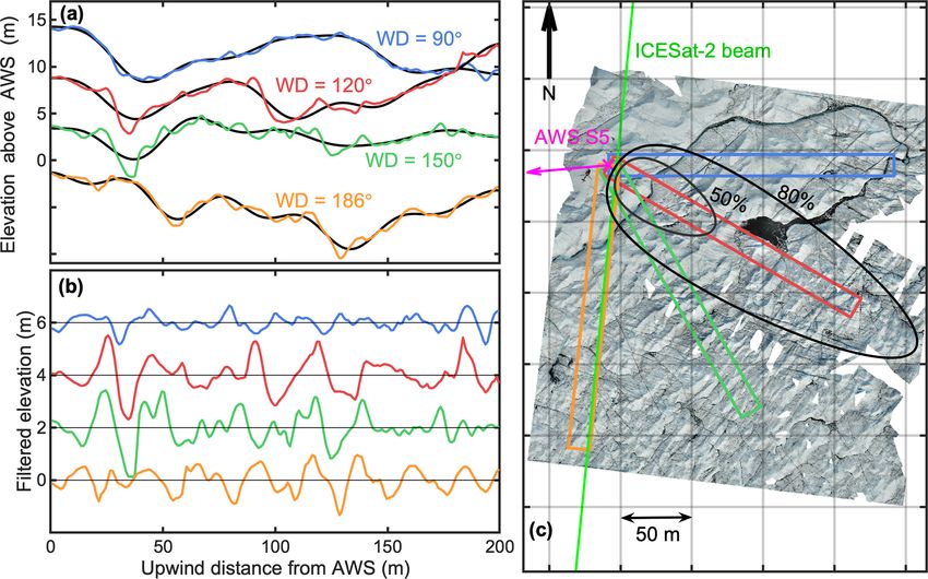
2604                                   M. van Tiggelen et al.: Mapping the Greenland Ice Sheet roughness using ICESat-2

point of interest (e.g. an automatic weather station, or AWS).      nal statistics are then computed using the first half of the fil-
This geometry is a strong simplification of the true fetch foot-    tered profile of length L. Typical filtered profiles are shown
print, which is calculated for a specific wind direction at S5      in Figs. 2b and 3. These profiles only contain the ice hum-
in Fig. 2, after Kljun et al. (2015). Yet this simplification al-   mocks, as the high-pass filter removed the influence of the
lows us to use 1D elevation datasets, such as profiles from         large-scale domes.
the ICESat-2 satellite laser altimeter. Besides, the true fetch        The height of the roughness obstacles (H ) is taken as
footprint depends on flow parameters such as the friction ve-
locity (u∗ ) and the boundary-layer height (Kljun et al., 2015),    H = 2e
                                                                         σz ,                                                    (5)
which are not known a priori.
                                                                    in which σez is the standard deviation of the filtered eleva-
   Four measured elevation profiles and a high-resolution
                                                                    tion profile. This is an arbitrary but convenient choice, as the
orthomosaic image are shown in Fig. 2. These were mea-
                                                                    standard deviation of the topography captures all the scales in
sured on 6 September 2019 at site S5 (67.094◦ N, 50.069◦ W,
                                                                    the filtered profile but remains insensitive to the height of the
560 m) in the locally prevailing wind directions, using UAV
                                                                    small-scale obstacles, which we assume to have a negligible
photogrammetry, of which the details will be given in Sect. 3.
                                                                    influence on the overall drag. Unfortunately, the variance is
At this site, pyramidal ice hummocks with heights between
                                                                    sensitive to the height of the largest obstacles and thus to the
0.5 and 1.5 m are superimposed on larger domes of more
                                                                    chosen value for 3.
than 50 m in diameter (see also Fig. 1b). The elevation pro-
                                                                       Next, we define an obstacle as a group of consecutive pos-
files for different fetch directions illustrate three important
                                                                    itive values of filtered heights, after Munro (1989) (see also
issues: (1) the zero-referencing of the surface, (2) the identi-
                                                                    Smith et al., 2016), which yields f , the number of obstacles.
fication of distinct roughness obstacles, and (3) the important
                                                                    The obstacle frontal area index (λ) in the direction of the el-
variability of the surrounding topography, depending on the
                                                                    evation profile is then computed as (Fig. 3)
fetch direction. The obstacles being anisotropic, the surface
appears rougher in the southerly directions than in the east-               Hw f H
erly directions. In addition, the ice ridges and troughs have       λ=f        =   ,                                             (6)
                                                                            Lw   L
variable heights and depths, which means that describing this
rough ice surface with a few length scales (e.g. H , λ) in order    where w is the width of the profile, set to 15 m. This value
to estimate the aerodynamic roughness will introduce some           was chosen to match the approximate ICESat-2 footprint di-
uncertainty. This is mainly because each individual obstacle        ameter, yet it is much smaller than the width of the real fetch
has a different contribution to the total drag. Unfortunately,      footprint (Fig. 2). We assume that the obstacles and the ele-
these individual drag contributions cannot be modelled, due         vation profile have the same width, which removes all infor-
to the unknown shape of the wind profile between the rough-         mation about the shape of the obstacles in the direction per-
ness elements. Without a universal theory of drag over com-         pendicular to the wind direction. This simplification avoids
plex surfaces, several simplifications need to be made.             the additional uncertainty regarding the aggregation of 2D
   We choose here to approximate the true surface as an array       datasets in the process of modelling z0m and allows us to ap-
of f identical obstacles of height H in the profile of length       ply the model to ICESat-2 profiles.
L (Munro, 1989; Smith et al., 2016) (Fig. 3). This avoids              To summarize, a measured elevation profile is now com-
the use of empirical formulas for the estimation of z0m and         pletely defined by the height of the obstacles (H ), and the
allows us to apply the bulk drag models. The approach of            frontal area index (λ), after high-pass filtering (see Fig. 3).
approximating a natural surface by uniquely shaped obsta-           This now allows us to apply a bulk drag model to estimate
cles is formally justified by Kean and Smith (2006), as most        one value for z0m per 200 m profile. The exact placement of
of the form drag is caused by the largest and steepest obsta-       the obstacles is resolved in the process (Fig. 3) but does not
cles. On the other hand, large natural obstacles also tend to be    serve as input for the drag models. Detailed equations of the
wide, so their relatively small frontal area index considerably     bulk drag model can be found in Appendix A.
reduces their contribution to the total form drag (Fitzpatrick
et al., 2019). To remove the influence of the widest obstacles,     3     Datasets
the elevation profile of length L is linearly detrended, and
the power spectral density of the detrended profile is com-         3.1    Eddy-covariance measurements
puted in order to filter out all the wavelengths larger than
the cutoff wavelength 3 = 35 m. This value is found to give         Vertical propeller eddy-covariance (VPEC; see also
optimal results, which is shown in Appendix B. In order to          T20) measurements are available at sites S5 (67.094◦ N,
avoid spectral leakage when applying Fourier statistics on          50.069◦ W, 560 m) and S6 (67.079◦ N, 49.407◦ W, 1010 m)
short and aperiodic signals, we extend each input profile with      since 2016, while AWS observations are available since
the identical but mirrored profile before computing the power       1993 and 1995 for each site (Smeets et al., 2018). For this
spectral density. This yields a symmetrical and thus periodic       study we use eddy-covariance measurements acquired dur-
profile of length 2L, which is then high-pass filtered. The fi-     ing September 2019 at site S5 and also site SHR (67.097◦ N,

The Cryosphere, 15, 2601–2621, 2021                                                     https://doi.org/10.5194/tc-15-2601-2021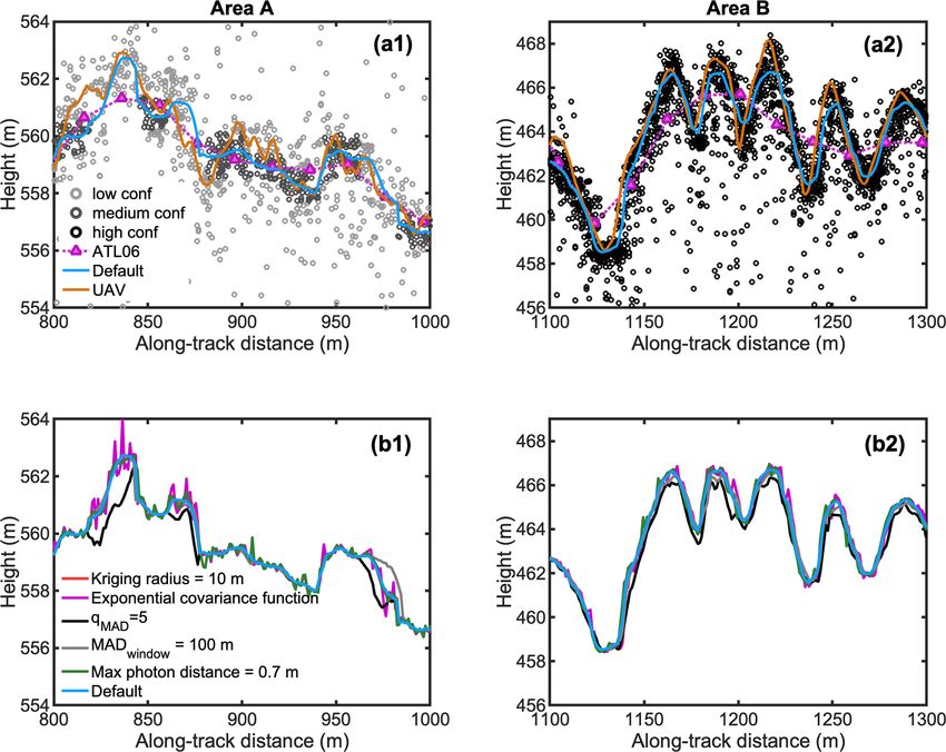
M. van Tiggelen et al.: Mapping the Greenland Ice Sheet roughness using ICESat-2                                                           2605

Figure 2. (a) Measured elevation profiles for four different wind directions upwind of AWS S5. (b) Filtered elevation profiles and (c) or-
thomosaic true-colour image of AWS S5 and surroundings taken by UAV photogrammetry on 6 September 2019. The different coloured
rectangles in (c) indicate the profiles shown in panel (a). The profiles have been vertically offset by 5 m in (a) and by 2 m in (b) for clarity.
The black line in (a) denotes the low-frequency contribution of the profiles for a cut-off wavelength 3 = 35 m. The pink arrow in (c) denotes
the displacement vector of the AWS between the ICESat-2 overpass on 14 March 2019 and the UAV imagery on 6 September 2019. The
estimated extent of the 50 % and 80 % fetch footprints for the data in September 2019 in a specific wind direction is shown by the black
ovals.

Figure 3. Steps in converting a measured digital elevation model to the modelled topography, where L is the length of the profile, f the
number of obstacles, H the height of the obstacles, and w the width of the elevation profile. The location and height of AWS S5 are shown
on top of the UAV elevation profile. The grey dots denote all the ATL03 photons, while the black dots denote the selected photons for the
kriging procedure. The solid blue line denotes the 1 m resolution interpolated profile for ATL03 data, and the pink dots denote the 20 m
resolution ATL06 signal.

https://doi.org/10.5194/tc-15-2601-2021                                                            The Cryosphere, 15, 2601–2621, 2021
2606                                      M. van Tiggelen et al.: Mapping the Greenland Ice Sheet roughness using ICESat-2

Table 1. Description of z0m in situ datasets on the K-transect. The data from Meesters et al. (1997), Smeets and Van den Broeke (2008),
Lenaerts et al. (2014), and Van Tiggelen et al. (2020) are denoted M97, SB08, L14, and T20 , respectively. The measurement methods are
(p) profile, (sec) sonic eddy covariance, or (vpec) vertical propeller eddy covariance.

  Site                                                                                      Reference           Data averaging
  (elevation)   Season     Surface type                       z0m range (m)                 (method)            period
  S5            Summer     densely packed ice hummocks,       6 × 10⁻³ –8 × 10⁻²            SB08 (p)            Sep 2003 & Aug 2004
  (550 m)                  between 0.5 and 1.5 m              1.79 × 10⁻³ –3.45 × 10⁻²      T20 (vpec)          Sep 2016
                                                              1.05 × 10⁻² –4.66 × 10⁻²      this study (sec)    Sep 2019
                Winter     snow and exposed ice hummocks      8 × 10⁻⁵ –1 × 10⁻³            SB08 (p)            Dec 2003–May 2004
                                                              2.9 × 10⁻⁴ –1.21 × 10⁻²       T20 (vpec)          Dec 2016–May 2017
  SHR           Summer     densely packed ice hummocks,       9.1 × 10⁻³ –4.38 × 10⁻²       this study (sec)    Sep 2019
  (710 m)                  between 0.5 and 1 m
  S6            Summer     sparse ice hummocks,               2 × 10⁻³ –2 × 10⁻²            SB08 (sec)          Sep 2003 & Aug 2004
  (1010 m)                 average height 0.6 m               1.26 × 10⁻³ –7.52 × 10⁻³      this study (vpec)   Aug 2019
                Winter     snow, sastrugi                     5 × 10⁻⁵ –6 × 10⁻⁴            SB08 (sec)          Dec 2003–May 2004
                                                              2 × 10⁻⁶ –1.33 × 10⁻⁴         this study (vpec)   Dec 2018–May 2019
  S9            Summer     changing from wet melting snow     2 × 10⁻⁶ –1 × 10⁻⁴            SB08 (p)            Sep 2003 & Aug 2004
  (1520 m)                 to large ice crystals              2 × 10⁻⁴ –5 × 10⁻⁴            M97 (sec)           July 1991
                Winter     snow, sastrugi                     2 × 10⁻⁵ –7 × 10⁻⁴            SB08 (p)            Dec 2003–May 2004
  S10           Summer     snow, sastrugi                     2 × 10⁻⁴ –7 × 10⁻⁴            L16 (sec)           Sep 2012
  (1880 m)

49.957◦ W, 710 m), and from September 2018 to Au-                     taken above the roughness layer, i.e. 9   \m (z) = 0. The latter is
gust 2019 at site S6. All these sites are situated in the lower       a reasonable assumption, given that the height of the obsta-
ablation area of the K-transect, which is a 140 km transect           cles (H ) at these sites is less than 1.5 m, which means that the
of AWS and mass balance observations on the western part              roughness layer unlikely exceeds 3 m (Smeets et al., 1999;
of the GrIS (van de Wal et al., 2012; Smeets et al., 2018).           Harman and Finnigan, 2007). On the other hand, when apply-
It extends from the ice edge up to 1850 m elevation and               ing the drag model to estimate z0m (Appendix A), the correc-
therefore covers many contrasting types of surfaces, ranging          tion factor 9\ m (z) is taken into account. The reason is that the
from the rough crevassed bare ice close to the ice edge, to the       obstacles are located in the roughness layer, where the verti-
year-round firn-covered surface at the highest locations (see         cal wind profiles deviate from the inertial sublayer wind pro-
Figs. 1 and 6). At the end of the melting season, the bare ice        files, according to Eq. (1). Details about the processing steps
surface at S5 and SHR is characterized by densely packed              and further data selection strategies can be found in T20.
hummocks up to 1.5 m height, while at S6 it is characterized          The data selection strategy removes all data points with wind
by more sparsely packed hummocks of 0.6 m average height.             directions outside the [80◦ ; 200◦ ] interval. In the following
The datasets include 30 min observations of the friction              sections we average ln(z0m ), which is of interest for the de-
velocity u∗ (z) and wind speed u(z) at the same height                termination of the vertical profile of horizontal wind speed
above the surface (z = 3.7 m). Two independent techniques             (Eq. 1). Additional in situ averaged z0m measurements ob-
were used at S5 and SHR. The first technique is the sonic             tained during different time periods and at several locations
eddy-covariance (SEC) method, which uses measurements                 along the K-transect are taken from Meesters et al. (1997,
from a sonic anemometer (CSAT3B, Campbell scientific,                 M97), Smeets and Van den Broeke (2008, SB08), Lenaerts
Logan, USA) sampled at 10 Hz. The second technique is the             et al. (2014, L14), and T20 and are summarized in Table 1.
VPEC method, which relies on measurements of a vertical
propeller, horizontal propeller, and fine-wire thermocouple           3.2   UAV structure from motion
sampled at 5 Hz. At S6, only the VPEC method was used
with a sampling interval of 4 s. For both methods, the
roughness length (z0m ) is calculated using Eq. (2).                  The high-resolution elevation maps are derived using a
   We only select data taken during near-neutral conditions           structure-from-motion workflow using UAV imagery. Two
(z/Lo < 0.1), and we assume that the measurements are                 crevassed areas close to the ice edge were mapped using
                                                                      an eBee fixed-wing UAV from Sensefly, while the area sur-

The Cryosphere, 15, 2601–2621, 2021                                                       https://doi.org/10.5194/tc-15-2601-2021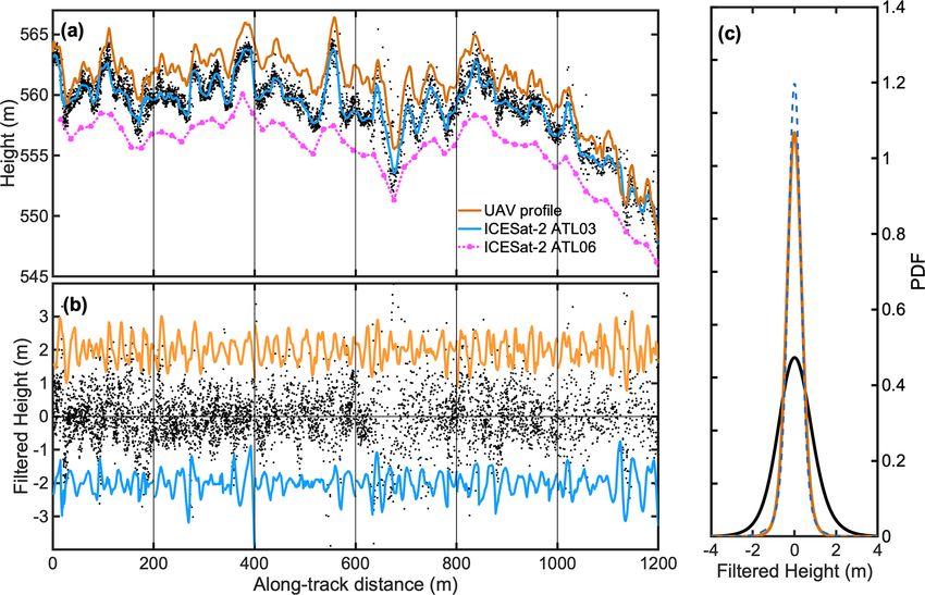
M. van Tiggelen et al.: Mapping the Greenland Ice Sheet roughness using ICESat-2                                                2607

rounding S5 was mapped using a Mavic Pro quadcopter UAV            which is not enough to apply the high-pass filter. And sec-
from DJI. Multiple overlapping true-colour images of the           ond, on this scale the number of roughness obstacles (f )
surface are processed in Agisoft Photoscan to produce 3D           would be greatly underestimated as can be seen in Figs. 3
elevation maps. Detailed information about this workflow           and 4. Fortunately, information smaller than the footprint di-
can be found in Immerzeel et al. (2014), Kraaijenbrink et al.      ameter can be extracted from the ATL03 product, as shown
(2016), and references therein. Briefly, the same surface fea-     by Herzfeld et al. (2020), in which a density–dimension al-
tures are identified on different images and are used to recon-    gorithm is used that facilitates surface height determination
struct the 3D geometry between the surface and the camera          at the 0.7 m nominal along-tack resolution. In the following
position. The resulting point cloud of the surface is then grid-   part we describe a method to produce a 1 m resolution along-
ded and finally geo-referenced using the information of the        track surface height estimation from the ATL03 raw photons
UAV GPS, which yields a digital elevation model (DEM) of           signal.
the surface. No additional ground-control points were used            The first step involves selecting all the ATL03 photons that
for the elevation maps, which is of little relevance in this       have been flagged as either low, medium, or high confidence
study, as we are not interested in the exact absolute eleva-       by the ATL03 algorithm. All the selected photons are pro-
tion but in relative obstacle heights. Details about the UAV       jected on the along-track segment, and a median absolute dif-
DEMs are provided in Table 2.                                      ference filter is used to remove all the photon heights which
   The elevation profiles are then extracted by projecting all     deviate too much from the local ensemble median,
the DEM points in a 200 m × 15 m rectangle on the centre                    qlow                           qhigh
line, followed by averaging the projected points in 1 m bins       hzi −          h|z − hzi|i ≤ z ≤ hzi +        h|z − hzi|i,    (7)
                                                                           0.6745                         0.6745
(see Fig. 3). The aim of this averaging method is to mimic
ICESat-2 profiles.                                                 where hzi denotes the median of z within a moving window.
                                                                   We choose qlow = 1 and qhigh = 2 in order to filter more pho-
3.3   ICESat-2 laser altimeter                                     tons below than above the median. We assume that the high-
                                                                   est detected photons are more likely to be first surface reflec-
Launched in September 2018 by the National Aeronautics             tions, while the lower photons are more likely to be delayed
and Space Administration (NASA), ICESat-2 (Ice, Cloud,             by scattering. We set the window length to 50 m. The pre-
and Elevation Satellite-2) carries a laser altimeter system in     vious selection strategy could also be applied for retrieving
near-polar orbit (Markus et al., 2017). The altimeter relies on    the surface in the case of multiple reflections (e.g. shallow
a photon-counting system, which in combination with both           supraglacial lakes), but this was not tested.
the spacecraft’s position and its pointing orientation, enables       The second step involves interpolating the irregular pho-
the retrieval of the 3-D position of individual backscattered      ton locations on a regular, 1 m resolution, along-track grid.
photons (Neumann et al., 2019). Our hypothesis is that the         The overlap between the individual footprints means that the
small footprint diameter (≈ 15 m) and short along-track spac-      geolocated photon heights in close vicinity must be corre-
ing between these footprints (0.7 m) allows for an accurate        lated to each other, with a correlation diameter similar to
estimation of land ice aerodynamic roughness properties.           twice the footprint diameter (≈ 30 m). We take advantage
   A typical geolocated photon measurement ATL03 (Neu-             of this feature to interpolate the ATL03 photons using a k-
mann et al., 2019) can be seen in Fig. 3 for site S5 and in        nearest neighbour, one-dimensional, ordinary kriging algo-
Fig. 4a for area A. Details about which ICESat-2 measure-          rithm, of which details can be found in Hengl (2009). In
ments are compared against the UAV surveys are provided in         essence, the interpolation weights depend on the covariance
Table 2. Not more than one ICESat-2 measurement exactly            with the nearby measurements, which is assumed to decrease
overlaps each UAV survey. This is mainly due to the presence       over distance. A Gaussian covariance function with a radius
of clouds and due to changes in laser pointing orientations        of 15 m is found to fit the experimental semi-variograms best.
in other ICESat-2 measurements, but also due to changes in         For computational efficiency, only the 100 closest geolocated
the studied locations due to ice flow. The global geolocated       photons within a quarter footprint diameter (3.75 m) of each
photon product ATL03 requires some processing steps be-            grid point are used for the interpolation. We only choose the
fore the roughness statistics can be computed. These steps         high confidence photons, but if there is less than 1 photon
mainly involve the selection of valid photons, aggregating         per 0.7 m, we also select the medium-confidence photons.
the 3-D photon positions on a regular along-track grid, and fi-    If there are not enough medium-confidence photons, we in-
nally correcting for remaining biases. The standard algorithm      crease the search radius to half the footprint diameter (7.5 m)
used to derive an accurate estimate of land ice height prod-       or even up to a footprint diameter (15 m). The low-confidence
uct from ATL03 to ATL06 is described in detail by Smith            photons are only used as a last resort. If in a 15 m footprint di-
et al. (2019). Unfortunately the 20 m along-track resolution       ameter there are still not enough photons present, the height
of the ATL06 land ice height product is too coarse for aero-       on that grid point is not estimated, which results in a gap. A
dynamic roughness calculations for two reasons. First, in the      sensitivity experiment using different photon selection strate-
ATL06 product there are only 10 points in 200 m sections,          gies and different kriging parameters is found in Appendix B.

https://doi.org/10.5194/tc-15-2601-2021                                                   The Cryosphere, 15, 2601–2621, 2021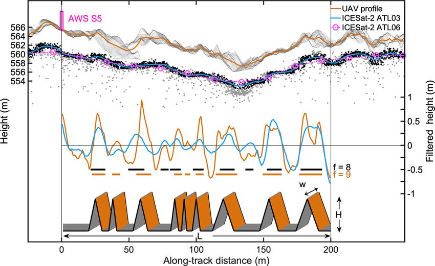
2608                                       M. van Tiggelen et al.: Mapping the Greenland Ice Sheet roughness using ICESat-2

Table 2. Description of DEMs obtained by UAV photogrammetry and of the corresponding overlapping ICESat-2 laser beams.

                                                                                                    ICESat-2
   Site    Centre coordinate          Dimensions (m)       Resolution (m)     UAV survey date       track-cycle-beam      ICESat-2 date
   A       67.171◦ N, 50.075◦ W           1500 × 1400                  0.3    1 September 2019      1169-04-gt1r          12 September 2019
   B       67.126◦ N, 50.075◦ W           2300 × 1300                 0.3     3 September 2019      1344-05-gt1r          23 December 2019
   S5      67.093◦ N, 50.065◦ W             450 × 375               0.025     6 September 2019      1169-02-gt1l          14 March 2019

Figure 4. (a) Elevation profile at site A measured by the UAV and by ICESat-2 (solid lines), selected ICESat-2 photons (black dots), and
ICESat-2 ATL06 height (pink dashed line). The UAV and ATL06 profiles have been vertically offset by 2 m for clarity. (b) Filtered profiles
(solid lines) and residual photon elevations after filtering per 200 m windows (grey dots), where the UAV and ATL03 filtered profiles have
also been vertically offset. (c) Probability density function of the filtered ICESat-2 profile (blue dashed line), UAV profile (orange solid line),
and residual photon elevations (black line).

   The last step involves grouping the interpolated eleva-                   obstacles. In addition, the frontal area index (λ) would re-
tion measurements in 200 m along-track windows and the                       main unknown.
high-pass filtering using a cut-off wavelength of 3 = 35 m                     When working with the 1 m interpolation profile, we
(Sect. 2). The height of the obstacles (H ) is defined as twice              model the standard deviation of the unresolved topography
the standard deviation of the filtered signal (Eq. 5).                       (σsub ) according to
   Although 1 m resolution is still too coarse to capture all the                                 0.5 .
                                                                                        2
small-scale obstacles that contribute to form drag, we expect                σsub = σph,res  − σi2        2,                          (8)
that most of the form drag over rough ice is caused by the
larger obstacles that are resolved by the ICESat-2 altimeter.                where σph,res is the standard deviation of the photon resid-
Furthermore, the small-scale information is still indirectly                 ual elevations, defined as the signal of the selected pho-
present in the scatter of the surrounding photons to the clos-               tons minus the interpolated 1 m resolution profile (Fig. 4),
est grid point, which is a measure of both the instrumental                  σi = 0.13 m is the standard deviation due to the instrumen-
error and the surface slope, but also of the surface roughness               tal precision (Brunt et al., 2019). We calculate σsub for each
(Gardner, 1982).                                                             200 m profile. The total variance of the surface elevation
   An alternative approach that does not require gridding the                measured by the laser altimeter in 200 m intervals is the sum
ATL03 product to 1 m resolution would be to use the stan-                    of both the resolved and unresolved variance:
dard deviation of the raw photon signal detrended for the re-                       q
                                                                             σtot = σ      2   2                                         (9)
solved 20 m resolution ATL06 data, as in Yi et al. (2005) and                         g res + σsub ,
Kurtz et al. (2008). However, as we will see in the following
                                                                             in which σres is the resolved standard deviation of the filtered
sections, this would overestimate the height of the roughness
                                                                                      g
                                                                             1 m resolution profile. The height of the roughness obstacles,

The Cryosphere, 15, 2601–2621, 2021                                                               https://doi.org/10.5194/tc-15-2601-2021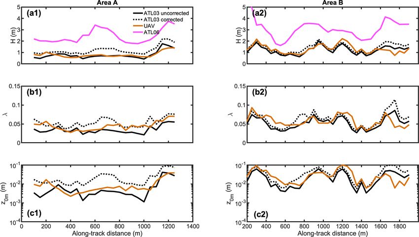
M. van Tiggelen et al.: Mapping the Greenland Ice Sheet roughness using ICESat-2                                                2609

corrected for the unresolved topography, is then estimated
according to

Hcorr = 2σtot .                                            (10)

The obstacle frontal area index (λ) is finally computed using
Eq. (6), where the number of obstacles (f ) is estimated from
the filtered profiles. Both H and λ are then used as input for
the bulk drag model (Appendix A), which results in one value
for z0m per 200 m profile.
   The filtered ICESat-2 signal and residual photon eleva-
tions at site A are shown in Fig. 4b, and their probability
density functions are shown in Fig. 4c. At this site, the fil-
tered ICESat-2 signal at 1 m resolution captures most of the
information present in the UAV signal. On the other hand,
the residual photon elevations, defined as the selected pho-
tons detrended for the interpolated profile under Eq. (9), still
contain much larger scatter than the UAV elevation profile.        Figure 5. Modelled z0m at site S5 using three different bulk drag
This demonstrates that roughness is not the only factor ex-        models, Lettau (1969, L69, blue lines), Macdonald et al. (1998,
plaining the scatter in the raw altimeter signal. Therefore us-    M98, green lines), and Raupach (1992, R92, red lines), and using
ing the residual scatter (Eq. 9) will overestimate the height      two different values for the drag coefficient for form drag: Cd =
of the roughness obstacles. In the next sections, we will anal-    0.25 (solid lines) and Cd = 0.1 (dashed lines). Solid grey sym-
yse the uncorrected height of the obstacles (H ), unless stated    bols are measurements from sonic eddy covariance (SEC) or ver-
otherwise.                                                         tical propeller eddy covariance (VPEC). Additional data are from
                                                                   Van Tiggelen et al. (2020, T20). Pink circles are the model results
                                                                   forced with H and λ from UAV photogrammetry, using the R92
4     Results                                                      model and Cd parameterized using Eq. (A2).

4.1    Evaluation of the bulk drag model forced with a
       UAV DEM
                                                                   for λ < 0.04 at this location (Fig. 5, blue line). In accor-
Bulk drag models are often used as a convenient way to esti-       dance with L69, the drag coefficient of an individual obstacle
mate the aerodynamic properties of natural surfaces. Never-        Cd = 0.25 is likely too high for naturally streamlined obsta-
theless, the number of quantitative evaluations of these mod-      cles. Furthermore, L69 does not consider the displacement
els for rough snow and ice surfaces is very limited. Brock         height, which means that the height of the obstacles (H )
et al. (2006) found that z0m modelled using the method by          relevant for form drag is overestimated. Nevertheless, L69
L69 (Eq. A13) agrees well with observations over melting           still yields a reasonable estimate of z0m for λ > 0.04, which
ice on a mountain glacier, although they used shorter pro-         can be explained by the neglect of the displacement that is
files, up to 15 m in length, and sampled in the orientation        compensated for by too small Cd for these fetch directions.
perpendicular to the wind direction. On the other hand, Van        The method by M98 (Eq. A14) does account for the dis-
den Broeke (1996) found that L69 overestimates z0m at site         placement height, and, while using the same drag coefficient
S4 at the K-transect (lowest site in Fig. 6). The same overes-     Cd = 0.25, it gives improved results for λ < 0.04 compared
timation was found by Smeets et al. (1999), Fitzpatrick et al.     to L69 (Fig. 5, green line). The same holds for the model by
(2019), and Chambers et al. (2019) for rough glacier ice but       R92 (Fig. 5, red line). M98 is expected to fail for very small
also by Miles et al. (2017) for a debris-covered glacier. These    λ, due to the absence of skin friction. Using Cd = 0.1, all
studies all use different methods at different sites to estimate   three models perform better for λ < 0.05 but perform poorly
H and λ, which illustrates the limited suitability of the model    for λ > 0.04 (Fig. 5, dashed lines). This is a strong indication
by L69 for realistic snow and ice surfaces.                        that Cd is not constant, but varies with the wind direction, de-
   To verify the suitability of several drag models (see Ap-       pending on the exact placement and shape of the obstacles.
pendix A), we use the eddy-covariance observations at site         In Sect. 4.3 we estimate the values for Cd required to fit the
S5 as independent validation (Sect. 3). Different values of        model to the observations; these values vary between 0.1 and
z0m are calculated for different fetch directions as depicted      0.3 and show a weak relationship with H . The parametriza-
in Fig. 2. Figure 5 compares both the estimated z0m from in        tion for Cd from Garbrecht et al. (1999) (Eq. A2), for which
situ observations and the modelled z0m at the end of the ab-       Cd increases with H , yields most acceptable results when
lation season, as a function of the measured obstacle frontal      used in combination with the R92 model (Fig. 5). Note that
area index λ. The L69 model (Eq. A13) overestimates z0m            Lüpkes et al. (2012) use a constant value for Cd .

https://doi.org/10.5194/tc-15-2601-2021                                                   The Cryosphere, 15, 2601–2621, 2021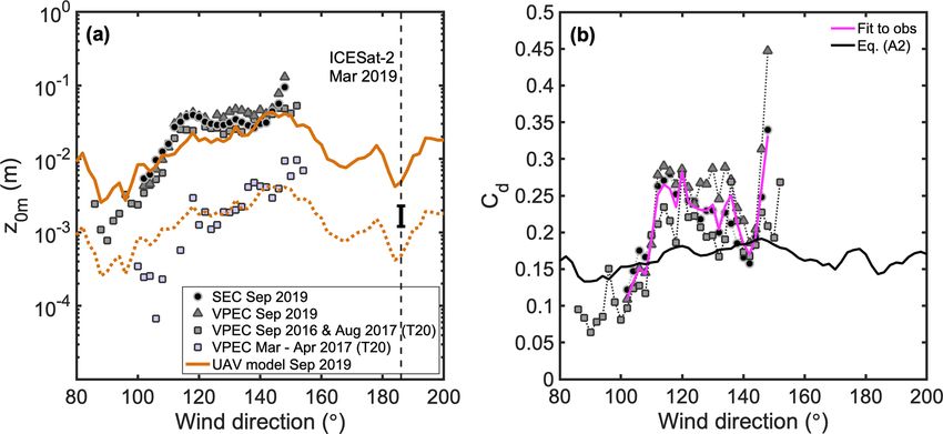
2610                                    M. van Tiggelen et al.: Mapping the Greenland Ice Sheet roughness using ICESat-2

Figure 6. Estimated height of the roughness obstacles (H ) from ICESat-2 between 16 October 2018 and 6 September 2020 in the lower part
of the K-transect, West Greenland. The locations of the automatic weather stations are given by the pink diamonds. The black boxes A and
B delineate the areas mapped by UAV photogrammetry. A hillshade of ArcticDEM (Porter et al., 2018) is shown as background over the ice
sheet.

   The R92 model with the parametrization for Cd allows for           ice edge. At first glance a clear pattern of roughness emerges,
some variability in modelled z0m for the same λ but is still not      in which ice dynamics and elevation seem to be the con-
able to reproduce the eddy-covariance observations (Fig. 5).          trolling factors. Low-lying bare-ice areas are rougher, while
We attribute this to the parametrization of Cd , which was            the higher, firn-covered areas are smooth. Nevertheless, the
derived for sea-ice pressure ridges and therefore likely less         roughness is very variable locally due to isolated crevasses
suitable for rough ice hummocks. Nevertheless, the overall            and melt channels. In addition, we expect a seasonal vari-
error between model and observation is acceptable, given the          ability that is not yet captured in this analysis.
simplicity of the bulk drag models that were designed for
idealized roughness geometries. As pointed out by L69, re-            4.3   Evaluation of ICESat-2 roughness statistics against
alistic modelling of total drag over a complex natural sur-                 UAV DEMs
face should intuitively require a complete variance spectrum
of the topography. Linking variance spectra to the total drag         Climate models and satellite altimeter corrections require in-
has been investigated recently through numerical simulations          formation about the larger-scale spatial variability of surface
(Yang et al., 2016; Zhu and Anderson, 2019; Li et al., 2020),         (aerodynamic) roughness. This motivated us to compare the
but a universal and physically based relationship for complex         roughness statistics acquired with high-resolution UAV pho-
surfaces is still lacking. In the next sections, we therefore use     togrammetry to the statistics estimated from the ICESat-2
the model of R92 with a parametrized Cd for mapping z0m               laser altimeter.
using either UAV or ICESat-2 profiles.                                   The elevation profile from the UAV survey in box A
                                                                      (Fig. 6) was already compared to the overlapping ICESat-
4.2    Height of the roughness obstacles (H) estimated                2 profiles in Fig. 4a, while H , λ, and z0m are compared in
       from ICESat-2                                                  Fig. 7. In box A, the UAV and ICESat-2 profiles were taken
                                                                      11 d apart at the end of the ablation season. The height (H )
The estimated height of the obstacles (H ) using 2 years              and frontal area index (λ) of the roughness obstacles are esti-
of ICESat-2 measurements (16 October 2018–6 Septem-                   mated for 200 m intervals, with each interval centre separated
ber 2020) crossing the lower part of the K-transect is shown          by 50 m. Overall, the uncorrected 1 m profile from ICESat-2
in Fig. 6. H ranges between less than 0.1 m at the higher lo-         (Fig. 7, solid black line) clearly captures all the largest ob-
cations and more than 3 m in rough crevassed areas near the           stacles and the large-scale variability but still slightly under-

The Cryosphere, 15, 2601–2621, 2021                                                        https://doi.org/10.5194/tc-15-2601-2021
M. van Tiggelen et al.: Mapping the Greenland Ice Sheet roughness using ICESat-2 2611 Figure 7. (a1, a2) Estimated height of the roughness obstacles (H ). (b1, b2) Estimated frontal area index. (c1, c2) Estimated aerodynamic roughness length (z0m ). (a1, b1, c1) Area A. (a2, b2 c2) Area B. The black lines denote the roughness statistics estimated from the ATL03 filtered profile, with or without accounting for the residual photon elevations (dashed and solid lines, respectively). The orange line denotes estimates using UAV elevation profiles, and the pink line denotes the height of obstacles estimated using the scatter of ATL03 photons detrended for the ATL06 signal. estimates both the height (H ) and the frontal area index (λ) In area B, crevassed and slightly rougher than A, the eleva- of the obstacles, compared to the UAV surveys (Fig. 7, or- tion was measured in December, 3 months after the UAV ange line). This is expected, given the size of the laser foot- survey. The uncorrected ICESat-2 profiles show a slightly print and the low-pass-filtering properties of the kriging pro- more pronounced underestimation of H compared to area A, cedure. On the other hand, the correction using the standard which we relate to snowfall reducing the height of the rough- deviation of the photon distribution (Eq. 9) overestimates H ness obstacles. On the other hand, the corrected ICESat- (Fig. 7, dashed black line). This can be explained by addi- 2 profiles overestimate H by 0.06 m, which translates into tional processes that affect the local photon distribution but an overestimation of z0m by approximately 2.5 × 10⁻³ m that we did not consider, such as the forward scattering in the (Fig. 7). On average, the uncorrected ICESat-2 values un- atmosphere (Kurtz et al., 2008), the penetration of photons derestimate z0m by 2.9 × 10−3 m for area A and 9 × 10⁻³ m in the ice layer (Cooper et al., 2021), or simply the presence for area B, which corresponds to ≈ 40 % and ≈ 36 % of the of outliers that passed the median absolute difference filter average z0m estimated by the UAV at these two sites. (Eq. 7). Furthermore, the obstacle frontal area index (λ) is At site S5, UAV elevation profiles and eddy-covariance underestimated by the ICESat-2 altimeter, since we do not measurements are available in September 2019, while the account for unresolved obstacles when counting the num- ICESat-2 elevation profile was measured in March (Table 2). ber of obstacles (f ). In addition, using the standard devia- Both the satellite and the UAV profiles are shown in Fig. 3. tions of the ATL03 product detrended for the 20 m resolu- Although the UAV profile is too short to statistically com- tion ATL06 signal results in an even greater overestimation pare H and λ to the ICESat-2 altimeter, the qualitative com- of H (Fig. 7, purple line). This is due to the fact that besides parison between the two confirms that the satellite altime- the additional processes broadening the altimeter signal, the ter is very capable of detecting most of the obstacles that scatter of this signal also contains the large-scale variability are smaller than 20 m in width. Interestingly, some depres- at wavelengths larger than 3 = 35 m. We assumed that such sions in the UAV DEM are not captured by ICESat-2, most large wavelengths can be neglected in the drag calculations; likely as a result of snow filling them in March. Furthermore, therefore they are removed in the filtered UAV and ICESat-2 the bending (or “doming”) of the UAV profile is visible near profiles. the edges, which is a consequence of the lack of reference Two more UAV surveys were performed in Septem- ground control points in the UAV data processing, which is ber 2019 in area B and around S5, but the overlapping a common issue with UAV data processing (James and Rob- ICESat-2 profiles were measured during winter (see Table 2). son, 2014). Both H and λ are smaller in the satellite profile The comparison of H , λ, and modelled z0m is given in Fig. 7. than in the UAV profile, but the modelled z0m agrees qualita- https://doi.org/10.5194/tc-15-2601-2021 The Cryosphere, 15, 2601–2621, 2021
2612                                      M. van Tiggelen et al.: Mapping the Greenland Ice Sheet roughness using ICESat-2

Figure 8. (a) Drag model evaluation at site S5. (b) Drag coefficient for form drag (Cd ) used in the bulk drag model (black line) or required to
perfectly fit the observations. The solid orange line is the modelled z0m using the R92 model and UAV photogrammetry on 6 September 2019,
while the dashed orange line is the orange line shifted down by a factor of 10. Solid symbols are measurements from sonic eddy-covariance
(SEC) or vertical propeller eddy-covariance (VPEC). Additional data are from Van Tiggelen et al. (2020, T20). The vertical dashed line
denotes the direction sampled by the ICESat-2 laser beam on 14 March 2019. The error bar denotes the range between the uncorrected and
corrected ICESat-2 measurements.

tively with that estimated using observations from the AWS                measurements. The difference in averaged estimated z0m us-
S5 during March–April. During this time period, z0m is ap-                ing in situ observations during the overlapping period across
proximately a factor of 10 smaller than during the end of the             all wind directions is 12 % between the VPEC and the SEC
ablation season (Fig. 8, dashed orange line). Unfortunately,              methods.
the track direction of the satellite altimeter rarely coincides              The ice hummocks seen in the easterly directions have
with the wind direction measured by the anemometers at this               smaller H and λ, which results in a smaller z0m than in
location, due to the katabatic forcing. This prevents a direct            the southerly directions. This is due to the anisotropic na-
comparison of ICESat-2 roughness to in situ observations, as              ture of the ice hummocks and is confirmed by the eddy-
the aerodynamic roughness strongly depends on the wind di-                covariance observations, regardless of the season. The extent
rection (Van Tiggelen et al., 2020). The z0m value estimated              of the UAV survey allows the application of the drag model
from ICESat-2 profiles must thus be interpreted as the aero-              for wind directions that rarely occur during the measurement
dynamic roughness in the wind direction along the direction               period. This is particularly useful for the development of z0m
of the ground laser track.                                                parametrizations in atmospheric models. Interestingly, the to-
   Only a high-resolution, two-dimensional DEM, e.g. ob-                  pography at site S5 translates into a wavy pattern of z0m as
tained using a UAV, allows for an accurate description of                 a function of wind direction, with two local minima at fetch
the aerodynamic roughness around a point of interest in mul-              directions of 90 and 180◦ (Fig. 8).
tiple directions. An example of such an analysis is shown                    To summarize, three independent but co-located meth-
for site S5 in Fig. 8. The R92 model applied to the UAV                   ods, namely UAV photogrammetry, ICESat-2 laser altimetry,
elevation profiles reproduces the considerable variability of             and in situ eddy-covariance measurements, allow us to es-
the estimated z0m using in situ observations. Across all the              timate the aerodynamic roughness of a rough ice surface at
wind directions available in the measurements, z0m using the              a specific site. The comparison confirms our two initial hy-
UAV profiles is underestimated by 7.6 × 10⁻³ m, or 28 % of                potheses: (1) the variability of estimated z0m using in situ
the average value estimated by the SEC method in Septem-                  observations as a function of wind direction found by T20
ber 2019 (2.65 × 10⁻² m). The comparison improves when                    is indeed a consequence of the anisotropic topography, and
comparing the modelled z0m to VPEC measurements from                      (2) the ICESat-2 data are very well suited to estimate z0m of a
September 2016 and August 2017 (T20), the model now                       rough ice surface in both space and time. Without correcting
overestimates the estimated z0m by in situ observations by                for the residual scatter in photon elevations, the 1 m resolu-
1.1 × 10⁻³ m or 9 % of the observed value (1.25 × 10⁻² m).                tion ICESat-2 profiles most likely provide a lower bound of
As these data contain more wind directions, the overestima-               roughness, as they underestimate z0m by almost a factor of 2
tion of z0m in the southerly fetch directions is compensated              at the two rough ice locations in areas A and B. On the other
for by an underestimation in the easterly directions (Fig. 8).            hand, an attempt to account for this residual scatter may lead
The difference between different in situ data highlights the              to an overestimated z0m , by a factor that depends on the noise
variability in z0m in time but also the uncertainty in the field          in the raw altimeter data. Nevertheless, given the fact that

The Cryosphere, 15, 2601–2621, 2021                                                             https://doi.org/10.5194/tc-15-2601-2021
M. van Tiggelen et al.: Mapping the Greenland Ice Sheet roughness using ICESat-2                                                   2613

Figure 9. Estimated aerodynamic roughness length (z0m ), without accounting for the residual photon backscatter, from ICESat-2 between
16 October 2018 and 6 September 2020 in the lower part of the K-transect, West Greenland. The locations of the automatic weather stations
are given by the pink diamonds. The black boxes A and B delineate the areas mapped by UAV photogrammetry. A hillshade of ArcticDEM
(Porter et al., 2018) is shown as background over the ice sheet.

z0m varies over several orders of magnitude, we deem this              while it is around 6 × 10⁻³ m during the other months. The
method useful to understand the spatio-temporal variability            average roughness approaches its minimum value of 10−4 m
of the aerodynamic roughness length over the GrIS.                     above 1000 m a.s.l., regardless of the time period. When the
                                                                       ICESat-2 altimeter does not detect any obstacle, the bulk
4.4   Results: mapping the roughness length z0m using                  drag model only accounts for skin friction, which is pre-
      ICESat-2                                                         scribed as a constant in the model. Interestingly, z0m de-
                                                                       creases very near the ice margin, which might be explained
                                                                       by the decreasing ice velocity at the margin, as most of the
In this section we apply the elevation profile filtering de-
                                                                       glaciers in this area are land-terminating.
scribed in Sect. 3 and the R92 model with parameterized Cd
                                                                          The measurements described in Table 1 are also included
(see Appendix A) to ICESat-2 ATL03 data to model and map
                                                                       in Fig. 10. The comparison indicates that the satellite product
the aerodynamic roughness (z0m ) over the K-transect. We
                                                                       captures the overall variability along the K-transect (Fig. 10).
process nearly 2 years of ICESat-2 ATL03 measurements,
                                                                       In particular at lower elevations, the modelled z0m is within
taken between 16 October 2018 and 6 September 2020. The
                                                                       the range of in situ observations. The in situ roughness z0m
results, without accounting for the unresolved photon scat-
                                                                       can vary due to changing wind direction, but also due to in-
ter, are presented in Fig. 9. Within a distance of 10 km from
                                                                       strumental uncertainty. Especially the smooth sites where the
the ice margin, z0m ranges between 10−3 and 10−1 m. There
                                                                       profile method has been used can exhibit large variability,
is a clear transition of z0m values that separates the rough
                                                                       such as at site S9 (see Table 1).
(S4, S5, KAN_L, SHR) and smooth (S6 and higher) surface
                                                                          Unfortunately, the ICESat-2 altimeter is not able to de-
in the ablation zone. Within a distance of several kilome-
                                                                       tect obstacles that contribute to form drag at sites S6
tres, z0m can vary by more than 1 order of magnitude, e.g.
                                                                       (1010 m a.s.l.) and higher. At S6, the surface is flat during
north of locations S5 and KAN_L (Fig. 9). In order to quan-
                                                                       winter but becomes rough during summer with ice hum-
tify the variability in time, we group the z0m values from
                                                                       mocks with 0.6 m average height (SB08). Unfortunately
ICESat-2 in two groups, July–September and October–June,
                                                                       the horizontal extent of these obstacles is smaller than the
which correspond to ICESat-2 cycles 1–3 & 5–8 and 4 &
                                                                       ICESat-2 footprint diameter (≈ 15 m). Higher up, the ice
8 respectively. The average z0m value for the two groups in
                                                                       hummocks become even smaller and the surface eventually
each 200 m elevation bin is presented in Fig. 10. During sum-
                                                                       becomes snow-covered year-round. Nevertheless, snow sas-
mer, the average z0m value is 1 × 10⁻² m below 600 m a.s.l.,

https://doi.org/10.5194/tc-15-2601-2021                                                      The Cryosphere, 15, 2601–2621, 2021
2614 M. van Tiggelen et al.: Mapping the Greenland Ice Sheet roughness using ICESat-2
Figure 10. Estimated aerodynamic roughness length (z0m ) from ICESat-2 between 16 October 2018 until 6 September 2020 along the K-
transect. The data were averaged over 200 m elevation bins and two time periods: summer (July–September) and winter (October–June). The
variability range denotes the two-sided standard deviation within one elevation class. The in situ observations are described in Table 1.
trugi, known to reach up to 0.5 m height at site S10 from the bulk drag partitioning model from Raupach (1992) such
photographic evidence, still contribute to form drag. This re- that it can be applied to 1D elevation profiles. Forcing this
sults in a maximum observed value of z0m = 7 × 10⁻⁴ m at model with 1 m resolution elevation profiles taken from the
sites S9 and S10 (Fig. 10). Using a rough estimate for both ICESat-2 satellite laser altimeter z0m becomes a quantifiable
H and λ at S6 and S10, based on photographs taken dur- and mappable quantity. The model assumes that the surface
ing the end of the ablation season, yields more realistic val- is composed of regularly spaced, identical obstacles, which
ues for z0m (Fig. A1) than using H and λ from the ICESat- all have the same drag coefficient. Despite the fact that the
2 elevation profiles. Therefore we conclude that the rough- drag coefficient for each individual obstacle remains poorly
ness obstacles are not properly resolved at these locations in known, the evaluation in this study against different in situ
the ATL03 data using the algorithm presented in this study, observations, using different techniques and for different lo-
even when the correction using the residual photon scatter cations and time periods, demonstrates the validity of this
is applied. This is mainly due to the limited footprint of the model. On the other hand, the use of the model of Lettau
ICESat-2 measurements, but also due to the orientation of (1969) is not recommended over a rough ice surface, as it
the surface features, which limits the detectability of highly does not separate the form drag and the skin friction and
anisotropic features from 1D profile measurements. These neglects both the effects of the displacement height and of
limitations in the ICESat-2 measurements result in a uniform inter-obstacle sheltering.
prescribed value of z0m = 1 × 10⁻⁴ m for elevations above Mapping surface obstacles at 1 m resolution using the
≈ 1000 m a.s.l. The algorithm described in Sect. 3 could be ICESat-2 altimeter data proves possible, as long as the rough-
adapted to extract these features from the ATL03 data. For in- ness obstacles are large enough (e.g. crevasses, ice hum-
stance, smaller-scale obstacles could be retrieved in multiple mocks). Obstacles that are small compared to the ICESat-2
directions at cross-over points, using the information from footprint diameter of ≈ 15 m, such as ice hummocks found
multiple ICESat-2 tracks. However, this is beyond the scope above 1000 m elevation in summer, or snow sastrugi ex-
of this study, which is to map the aerodynamic roughness of pected year-round at even higher locations on the ice sheet
rough ice at large scales. from photographic evidence, are not resolved by the ICESat-
For now, the implications of these findings for the sensi- 2 measurements when used in combination with the methods
ble heat flux, and thus surface ablation, remain to be investi- presented in this study. This translates into a lower bound
gated. The areas with high z0m are in the low-lying ablation of z0m ≈ 10−3 m that can realistically be mapped using this
zone close to the ice edge, where the highest melt rates are method. Furthermore, accounting for the scatter in the unre-
observed. Accounting for the variable roughness might shed solved altimeter signal leads to overestimates of the aerody-
light on the drivers of these high melt rates. namic roughness, as this scatter is a consequence of many
different processes that must individually be modelled.
The methods presented in this paper can effectively be
5 Conclusions used to map z0m at ice sheet elevations below 1000 m. This
lower ablation area is also where the contribution of turbu-
The aerodynamic roughness of a surface (z0m ) in part de-
lent heat fluxes to surface ablation, and thus runoff, is the
fines the magnitude of the surface turbulent energy fluxes, yet
largest. As a consequence of the orientation of the ICESat-2
is often poorly known for glaciers and ice sheets. We adapt
The Cryosphere, 15, 2601–2621, 2021 https://doi.org/10.5194/tc-15-2601-2021You can also read