The retrieval of snow properties from SLSTR Sentinel-3 - Part 1: Method description and sensitivity study
←
→
Page content transcription
If your browser does not render page correctly, please read the page content below
The Cryosphere, 15, 2757–2780, 2021
https://doi.org/10.5194/tc-15-2757-2021
© Author(s) 2021. This work is distributed under
the Creative Commons Attribution 4.0 License.

The retrieval of snow properties from SLSTR Sentinel-3
– Part 1: Method description and sensitivity study
Linlu Mei, Vladimir Rozanov, Christine Pohl, Marco Vountas, and John P. Burrows
Institute of Environmental Physics, University of Bremen, Bremen, Germany

Correspondence: Linlu Mei (mei@iup.physik.uni-bremen.de)

Received: 16 September 2020 – Discussion started: 7 October 2020
Revised: 12 March 2021 – Accepted: 22 March 2021 – Published: 18 June 2021

Abstract. The eXtensible Bremen Aerosol/cloud and sur-             tion due to unperfected atmospheric correction and cloud
facE parameters Retrieval (XBAER) algorithm has been de-           screening introduces underestimation of SGS, “inaccurate”
signed for the top-of-atmosphere reflectance measured by           SPS and overestimation of SSA; (6) the impact of the instru-
the Sea and Land Surface Temperature Radiometer (SLSTR)            ment spectral response function introduces an overestimation
instrument on board Sentinel-3 to derive snow properties:          into retrieved SGS, introduces an underestimation into re-
snow grain size (SGS), snow particle shape (SPS) and spe-          trieved SSA and has no impact on retrieved SPS; and (7) the
cific surface area (SSA) under cloud-free conditions. This is      investigation, by taking an ice crystal particle size distribu-
the first part of the paper, to describe the retrieval method      tion and habit mixture into account, reveals that XBAER-
and the sensitivity study. Nine pre-defined SPSs (aggregate        retrieved SGS agrees better with the mean size, rather than
of 8 columns, droxtal, hollow bullet rosette, hollow column,       with the mode size, for a given particle size distribution.
plate, aggregate of 5 plates, aggregate of 10 plates, solid bul-
let rosette, column) are used to describe the snow optical
properties. The optimal SGS and SPS are estimated itera-
tively utilizing a look-up-table (LUT) approach. The SSA           1   Introduction
is then calculated using another pre-calculated LUT for the
retrieved SGS and SPS. The optical properties (e.g., phase         Snow properties such as snow albedo, snow grain size (SGS),
function) of the ice crystals can reproduce the wavelength-        snow particle shape (SPS), specific surface area (SSA) and
dependent and angular-dependent snow reflectance features,         snow purity (Warren and Wiscombe, 1980; Painter et al.,
compared to laboratory measurements. A comprehensive               2003; Hansen and Nazarenko, 2004; Taillandier et al., 2007;
study to understand the impact of aerosols, SPS, ice crystal       Gallet et al., 2009; Battaglia et al., 2010; Gardner and Sharp,
surface roughness, cloud contamination, instrument spectral        2010; Domine et al., 2011; Liu et al., 2012; Qu et al., 2015;
response function, the snow habit mixture model and snow           Baker, 2019; Pohl et al., 2020a) show large variabilities tem-
vertical inhomogeneity in the retrieval accuracy of snow           porally and spatially (Kukla et al., 1986). They play impor-
properties has been performed based on SCIATRAN radia-             tant roles in the global radiation budget, which is critical to
tive transfer simulations. The main findings are (1) snow an-      some well-known phenomena such as Arctic amplification
gular and spectral reflectance features can be described by        (Serreze and Francis, 2006; Domine et al., 2019). Satellites
the predefined ice crystal properties only when both SGS and       offer an effective way to understand the surface–atmosphere
SPS can be optimally and iteratively obtained; (2) the im-         processes and corresponding feedback mechanisms on the
pact of ice crystal surface roughness on the retrieval results     regional, continental and/or global scales (Konig et al., 2001;
is minor; (3) SGS and SSA show an inverse linear relation-         Pope et al., 2014). Satellite-derived snow products (e.g.,
ship; (4) the retrieval of SSA assuming a non-convex particle      SGS, SPS and SSA) are particularly important for short-
shape, compared to a convex particle shape (e.g., sphere),         term hydrological, meteorological and climatological model-
shows larger retrieval results; (5) aerosol/cloud contamina-       ing (Livneh et al., 2009). A high-quality snow property data
                                                                   product can also be applied to derive aerosol optical thick-

Published by Copernicus Publications on behalf of the European Geosciences Union.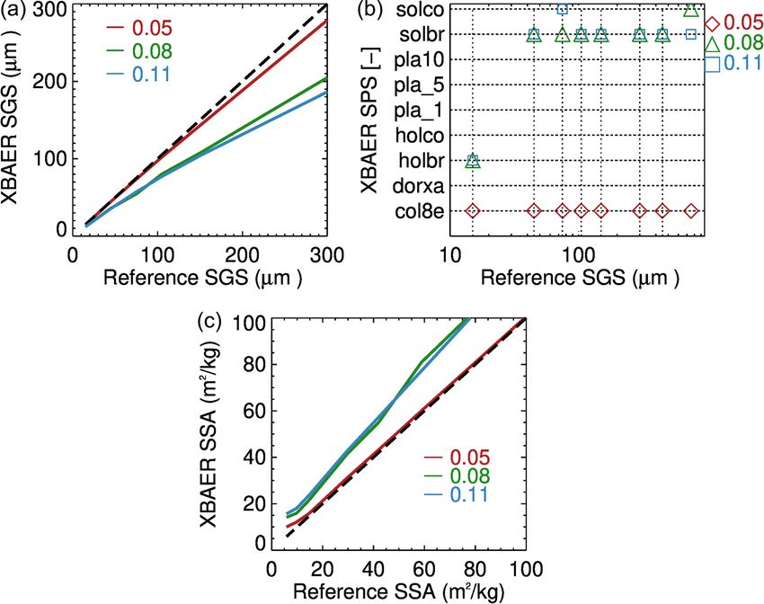
2758                                                                L. Mei et al.: Retrieval of snow properties from SLSTR

ness (AOT) over the cryosphere (Mei et al., 2020a). High-          2013). Improper wavelength-dependent snow bidirectional
quality satellite-derived snow products and their by-products      reflectance caused by a predefined SPS leads to low-quality
are also important for the creation of long-term climate data      satellite retrieval results. Some attempts to derive SPS in the
records (SSMC, 2014), which enable better investigation and        ice cloud can be found in previous publications (McFarlane
interpretation concerning global climate change (Konig et al.,     et al., 2005; Cole et al., 2014).
2001). However, both the definition and the corresponding             According to Legagneux et al. (2002), SSA is defined as
data accuracy of SGS are poor (Langlois et al., 2020), and         the surface area of ice crystal per unit mass; i.e., SSA =
there is no existing SPS satellite product. The lack of good       At /ρV , where At and V are total surface area and volume,
information on SGS and SPS leads to a low quality of SSA           respectively, and ρ is the ice density. SSA includes informa-
(Gallet et al., 2009). The accuracy of SGS, SPS and SSA lim-       tion on both SGS and SPS, and it is often used to describe the
its the model performance for the prediction of snow proper-       surface area available for chemical processes (Taillandier et
ties related to climate change issues. Lack of information on      al., 2007; Domine et al., 2011; Yamaguchi et al., 2019). SSA
SGS and SPS also restricts the accuracy of snow bidirectional      is reported to have a good relationship with snow spectral
reflectance estimation, which further limits the retrieval pos-    albedo at the shortwave infrared wavelengths (Domine et al.,
sibilities of aerosol and cloud properties above snow (Mei et      2007). Optical methods are routinely used to measure SSA
al., 2020a, b).                                                    in the field (Gallet et al., 2009). Empirical equations have
   A comprehensive overview of remote sensing of SGS, SPS          been proposed to describe the change in SSA (Legagneux
and SSA can be found in many previous publications (e.g.,          and Domine, 2005; Taillandier et al., 2007). Few attempts
Li et al., 2001; Stamnes et al., 2007; Koren, 2009; Lya-           have been made to derive SSA from satellite observations
pustin et al., 2009; Dietz et al., 2012; Wiebe et al., 2013;       (Mary et al., 2013; Xiong et al., 2018).
Frei et al., 2012; Mary et al., 2013; Kokhanovsky, et al.,            This paper presents a new retrieval algorithm to derive
2019; Xiong and Shi, 2018). The variation in SGS leads to          SGS, SPS and SSA from satellite observations. In a snow–
the large variability in top-of-atmosphere (TOA) reflectance       atmosphere system, satellite-observed TOA reflectances are
in near-infrared (NIR)/shortwave infrared (SWIR) spectral          affected by numerous snow and atmospheric parameters. The
ranges, and SPS shows a strong impact on TOA reflectance           parameters, which will be estimated in the framework of the
in visible channels (Warren and Wiscombe, 1980). Differ-           eXtensible Bremen Aerosol/cloud and surfacE parameters
ent retrieval algorithms have been developed for different         Retrieval (XBAER) algorithm, will be called the target pa-
instruments. For instance, the MODIS Snow-Covered Area             rameters. Other parameters, which the TOA reflectance also
and Grain size (MODSCAG) retrieval algorithm and Multi-            depends on, will be called the model parameters. In the case
Angle Implementation of Atmospheric Correction (MAIAC)             of the XBAER algorithm, the target parameters are SGS, SPS
algorithm have been used to derive SGS using MODIS and             and SSA, whereas the model parameters are aerosol loading,
VIIRS instruments (Painter et al., 2003, 2009; Lyapustin et        cloud optical thickness and gaseous absorption. Throughout
al., 2009).                                                        the paper, SGS will be characterized by an effective radius.
   Snow particle shape is another important parameter which        Following Baum et al. (2011), the effective radius is defined
affects the estimation of snow properties, such as albedo          as 3V /(4Ap ), where V and Ap are the volume and average
(Räisänen et al., 2017; Flanner and Zender, 2006), because         projected area, respectively. As can be seen in the case of a
ice crystals with different shapes have different optical prop-    spherical particle, the effective radius is equal to the radius of
erties (Jin et al., 2008; Yang et al., 2013). The absorption       the sphere. The general concept of the retrieval algorithm is
and extinction cross sections of an ice crystal can be de-         to use simultaneously spectral and angular reflectance mea-
scribed as a function of size, shape, and the refractive in-       surements, which are sensitive to SGS and SPS. The spec-
dex at a given wavelength (van de Hulst, 1981; Mischenko           tral channels used in the XBAER algorithm are 0.55 and
et al., 2002, and references therein). Natural snow consists       1.6 µm. Both nadir and oblique observation directions from
of grains, depending on temperature, humidity and meteo-           the Sea and Land Surface Temperature Radiometer (SLSTR)
rological conditions, which have numerous different shapes         are used. An optimal SGS and SPS pair is achieved by
(Nakaya, 1954). SPSs have been classified into different cate-     minimizing the difference between measured and simulated
gories; the classification has been increased from 21 (Nakaya      atmosphere-corrected surface reflectances. SSA is then cal-
and Sekido, 1938) to 121 (Kikuchi et al., 2013) categories.        culated based on the retrieved SGS and SPS. Nine predefined
Although a spherical-shape assumption is typically used for        SPSs (aggregate of 8 columns, droxtal, hollow bullet rosette,
field measurements (Flanner and Zender, 2006; Donahue et           hollow column, plate, aggregate of 5 plates, aggregate of 10
al., 2020), this approximation is not recommended to be used       plates, solid bullet rosette, column) (Yang et al., 2013; see
in retrieval algorithms of satellite measurements because it       Table 1) are used to describe the snow optical properties and
leads to large differences between observed and simulated          to simulate the snow surface reflectance at 0.55 and 1.6 µm
wavelength-dependent snow bidirectional reflectance, espe-         at two observation angles.
cially at visible wavelengths (Leroux and Fily, 1998; Aoki et
al., 2000; Jin et al., 2008; Dumont et al., 2010; Libois et al.,

The Cryosphere, 15, 2757–2780, 2021                                                    https://doi.org/10.5194/tc-15-2757-2021
L. Mei et al.: Retrieval of snow properties from SLSTR                                                                             2759

Table 1. Snow particle shape provided in Yang et al. (2013) database. The abbreviations introduced here will be used later.

                                      Snow particle shape         Abbreviation    Schematic drawing

                                      Aggregate of 8 columns      col8e

                                      Droxtal                     droxa

                                      Hollow bullet rosette       holbr

                                      Hollow column               holco

                                      Plate                       pla_1

                                      Aggregate of 5 plates       pla_5

                                      Aggregate of 10 plates      pla_10

                                      Solid bullet rosette        solbr

                                      Column                      solco

   There are three points we would like to emphasize to                       sonal communication, 2021). In a field measurement
avoid misunderstandings between the snow science commu-                       and its related application areas (e.g., calculation of
nity and remote sensing community.                                            snow albedo), a spherical-shape assumption is widely
  – Usage of the Yang et al. (2013) database for ice crys-                    used because it is easier to derive other snow proper-
    tals in the air (ice cloud) and on the ground (snow). The                 ties such as SSAs and snow albedo based on this as-
    optical properties of ice crystals presented by Yang et                   sumption, compared to using other more complicated
    al. (2013) have been widely used to study ice clouds.                     shapes (see Appendix). The assumptions of a spherical
    In recent publications, it has been demonstrated that                     and non-spherical shape have much less impact on the
    they can also be used for snow studies (Räisänen et al.,                  estimation of snow albedo compared to the bidirectional
    2015; Pirazzini et al., 2015; Saito et al., 2019; Schnei-                 reflection features of snow (Grenfel and Warren, 1999;
    der et al., 2019; Pohl et al., 2020b). In fact, the single-               Dumont et al., 2010), because SPS has a significant im-
    scattering properties of ice crystals in the Yang et al.                  pact on the ice crystal phase function while it has a rela-
    (2013) database are determined solely by the given par-                   tively weak impact on the snow extinction/absorption
    ticle size, shape and refractive index. They can be used                  coefficient (Jin et al., 2008). However, the spherical
    to describe the optical properties of both snow parti-                    shape cannot be used to provide typical bidirectional re-
    cles and ice cloud particles when the particle models                     flection features of snow with the required accuracy (Jin
    represent the aforementioned optical/physical proper-                     et al., 2008; Dumon et al., 2010; Jiao et al., 2019), which
    ties (Saito et al., 2019; Masanori Saito, personal com-                   is the fundamental basis for deriving snow properties
    munication, 2021).                                                        from satellite remote sensing techniques. Thus, more
                                                                              complicated SPSs, such as those proposed by Yang et
  – Snow particle shape observed from field measurements                      al. (2013), are recommended to use in the simulations
    and derived from satellite observations. For scientists                   of the angular distribution of snow reflectance. Besides,
    working in a laboratory or on campaign-based stud-                        both snow albedo and directional reflectance are af-
    ies, the best way to obtain an image of snow is to use                    fected by other factors such as how single particles ag-
    an X-ray microtomography or confocal scanning opti-                       gregate.
    cal microscope/scanning electron microscope (Hagen-
    muller et al., 2016; Baker et al., 2019; Ian Baker, per-

https://doi.org/10.5194/tc-15-2757-2021                                                         The Cryosphere, 15, 2757–2780, 2021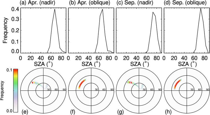
2760                                                                  L. Mei et al.: Retrieval of snow properties from SLSTR

    – SGS and SSA. Although what the definition of a snow
      grain constitutes is an ongoing debate in different com-
      munities, SGS and SPS are two fundamental inputs for
      any radiative transfer model, which is the basis for the
      satellite retrievals (Langlois et al., 2020). Typically, the
      SSA is preferable within the snow science community
      because SSA is commonly used in further applications
      based on field measurements. We note, however, ac-
      cording to the definition of SSA, for a given SPS, a
      unique relationship between SGS and SSA can be de-
      rived. SPS is the intermediate but fundamental parame-
      ter needed to retrieve SSA in our XBAER algorithm.
                                                                     Figure 1. Upper panels are the histograms of SZA for SLSTR ob-
   This paper is structured as follows: observation character-       servations: (a) nadir during April, (b) oblique during April, (c) nadir
istics of SLSTR and the laboratory measurements used for             during September, and (d) oblique during September. Lower panels
sensitivity studies are described in Sect. 2. The theoretical        are the polar plots of (VZA, RAA) probability for AATSR obser-
background and the ice crystal database (Yang et al., 2013)          vations: (e) nadir during April, (f) oblique during April, (g) nadir
are presented in Sect. 3. Section 4 describes the eXtensi-           during September, and (h) oblique during September.
ble Bremen Aerosol/cloud and surfacE parameters Retrieval
(XBAER) algorithm. The results of a comprehensive sensi-
tivity study using SCIATRAN (Rozanov et al., 2014) simu-             tical analysis has been performed using observations made
lations are presented in Sect. 5. The conclusions are given in       over Greenland during April and September 2017. April and
Sect. 6.                                                             September are reported to be representative months of the
                                                                     Arctic (Mei et al., 2020a). Please note that these two months
                                                                     are picked to represent the SLSTR observation characteris-
2     Data                                                           tic with a typical solar illumination angle; the change in un-
                                                                     derlying surface properties plays no role in such a selection.
2.1    SLSTR instrument                                              Figure 1 shows the frequency of SLSTR observation geome-
                                                                     tries. The upper panels show the SZA with SLSTR nadir
The satellite data will be used in two ways throughout the two       and oblique observations for April and September. We can
companion papers (this paper and Mei et al., 2021). In the           see that the SZA occurs frequently with a value of 70◦ for
first part, we perform a statistical analysis of the SLSTR ob-       selected months. The VZA and RAA for oblique observa-
servation/illumination geometries to select realistic settings       tion mode are typically around 55◦ and in a range of [110◦ ,
for the sensitivity study. In the companion paper, the satellite     170◦ ], respectively. The observation geometries for nadir
measurements will be used as the inputs of the XBAER al-             observation show relatively large variabilities due to larger
gorithm to derive the research satellite products of SGS, SPS        swath width compared to for oblique observations (1400 vs.
and SSA.                                                             700 km). Larger SZAs can be found especially at the edge of
   The SLSTR instrument on board the European Space                  the swath. The VZA and RAA for oblique observation mode
Agency (ESA) satellite Sentinel-3 is the successor of the Ad-        are typically in ranges of [0◦ , 55◦ ] and [70◦ , 140◦ ], respec-
vanced Along-Track Scanning Radiometer (AATSR) instru-               tively. According to the statistical analysis, a combination of
ment and is used to maintain continuity with the (A)ATSR             SZA, VZA and RAA of 70, 30 and 135◦ for nadir observa-
series of instruments. SLSTR has the heritage of AATSR               tion and 70, 55 and 135◦ for oblique observation can be a
instrument characteristics, especially the dual-viewing ob-          reasonable setting for the SLSTR observation geometries for
servation capabilities and wavelength settings. In order to          the sensitivity study.
have a reasonable setting for observation/illumination ge-
ometries in the sensitivity study, we perform a statistical          2.2   Laboratory measurements
analysis of the SLSTR observation geometries (solar zenith
angle, SZA; viewing zenith angle, VZA; relative azimuth              Laboratory measurements of the bidirectional reflectance of
angle, RAA), similarly to Mei et al. (2020a). This analy-            snow samples contain important information about the de-
sis is essential because (1) it provides a realistic setting of      pendence of the angular structure of snow reflection on the
observation/illumination geometries in our sensitivity stud-         lighting geometry, wavelength and snow physical properties.
ies and (2) it helps us to have a complete understanding             The comparison of measured and modeled bidirectional re-
of the observation-/illumination-related surface/atmospheric         flectance helps to establish the conceptual ideas for the re-
properties. Here the definition of RAA has been harmonized           trieval algorithm. For this comparison, we have selected mea-
with SCIATRAN (Rozanov et al., 2014); namely, the RAA                surements of fresh and aged snow samples presented by Du-
value is equal to 0◦ under a strict glint condition. The statis-     mont et al. (2010) and Peltoniemi et al. (2009), respectively.

The Cryosphere, 15, 2757–2780, 2021                                                        https://doi.org/10.5194/tc-15-2757-2021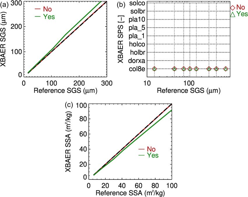
L. Mei et al.: Retrieval of snow properties from SLSTR                                                                    2761

   The fresh snow sample, a cylinder of 30 cm diameter and         diative transfer package SCIATRAN (Rozanov et al., 2014).
12 cm height, was taken from a new wet snow layer at Col           The snow layer was defined as a layer directly over a black
de Porte (Chartreuse, France) at 1300 m above sea level dur-       surface, with snow optical thickness of 500 and a snow ge-
ing January 2008 (Dumont et al., 2010). The sample was             ometrical thickness of 1 m. The snow layer is assumed to
stored in a cold room at −10 ◦ C for 1 week to avoid meta-         be vertically and horizontally homogeneous without any sur-
morphic effects during the ensuing measurements. To obtain         face roughness and composed of monodisperse ice crystals.
the bidirectional reflectance factor (BRF), the snow sample        The impact of snow impurities and scattering/absorption pro-
was illuminated by a monochromatic light source at an in-          cesses in the atmosphere was neglected at this stage. The
cidence zenith angle of 60◦ . The spectral BRF between 500         reflectance of the snow layer as a function of the effective
and 2600 nm was measured at viewing zenith angles of 0, 30,        radius of ice crystals at wavelengths of 0.55 and 1.6 µm is
60, and 70◦ and relative azimuth angles 0, 45, 90, 135, and        presented in Fig. 2. The calculations were performed for typ-
180◦ by a spectrogonio radiometer developed at the Labora-         ical SLSTR instrument observation/illumination geometries
toire de Planétologie de Grenoble, France, and using a Spec-       (see Sect. 2.1), with SZA, VZA and RAA equal to 70, 30 and
tralon® and an Infragold® sample as a reference (see Du-           135◦ (scattering angle 129◦ ).
mont et al., 2010, for further details).                              There are a couple of criteria we considered for the se-
   The aged snow sample, a cuboid of more than 10 cm               lection of the optimal wavelengths (0.55 and 1.6 µm) in the
height, was taken from an old dry snow layer at Masala,            XBAER algorithm, for the purpose of creating a long-term
Finland, and brought into a warm laboratory. The spectral          satellite snow property dataset with good and stable accu-
BRF between 350 and 2500 nm was measured during the                racy.
aged process by the Finnish Geodetic Institute field go-
                                                                     – We took the overlap channels between AATSR and
niospectropolariphotometer (FIGIFIGO) and using a Lab-
                                                                       SLSTR because a consistent long-term satellite snow
sphere Spectralon® 99 % white reference plate. For illumina-
                                                                       dataset is possible only when the same algorithm can
tion, a 1000 W Oriel Research quartz tungsten halogen lamp
                                                                       be applied to both AATSR and SLSTR instruments. In
at a zenith angle of 60◦ was utilized (Peltoniemi et al., 2009).
                                                                       particular, the overlap channels between AATSR and
The spectral BRF was obtained at viewing zenith angles of
                                                                       SLSTR are 0.55, 0.66, 0.87, 1.6, 3.7, 10.85 and 12 µm.
up to 70◦ in 1◦ resolution and at relative azimuth angles of 0,
90, 130, 160, 180, 270, 310 and 340◦ . The first and last mea-       – Picking up wavelengths for which the contribution of
surements were made in the principal plane, indicating minor           thermal emission can be ignored, then 0.55, 0.66, 0.87
metamorphism in the snow layer during the measurement.                 and 1.6 µm remain.
                                                                     – Deleting the channel 0.66 µm to avoid the potential im-
3   Dependence of snow reflectance on target parameters                pact of O3 absorption, after that, 0.55, 0.87 and 1.6 µm
                                                                       remain.
A comprehensive data library (Yang et al., 2013) containing
                                                                     – We take into account that the retrieval algorithm is a
the scattering, absorption and polarization properties of ice
                                                                       two-stage algorithm; namely, first it uses channels with
particles in the spectral range from 0.2 to 15 µm was used to
                                                                       minimum impact of the ice crystal shape to retrieve the
calculate radiative transfer through a snow layer (Pohl et al.,
                                                                       grain size, and then it selects the shape using channels
2020b). A full set of single-scattering properties is available
                                                                       with minimum impact of grain size. Accounting for the
for nine ice crystal habits presented in Table 1. The maximum
                                                                       fact that the 0.87 µm channel is impacted by both size
dimension of each habit ranges from 2 to 10 000 µm in 189
                                                                       and shape, 0.55 and 1.6 µm channels were picked up for
discrete sizes.
                                                                       the retrieval.
   The optical properties of ice crystals depend on wave-
length, ice crystal size and shape. Maximal dependence of             The right panel of Fig. 2 demonstrates the strong de-
the single-scattering albedo on the particle size is observed      pendence of the snow layer reflectance at 1.6 µm on the
in the spectral ranges where ice absorption cannot be ne-          SGS. One can also see that the dependence of snow re-
glected. The asymmetry factor depends on the particle size         flectance on SPS cannot be neglected. In particular, the same
for the whole spectral range. This dependence can be weaker        reflectance can be obtained with a combination of differ-
or stronger at a selected wavelength depending on SPS (see         ent SGS and SPS. For instance, one can see from the right
Yang et al., 2013, for details).                                   panel of Fig. 2 that the reflectance of the snow layer con-
   To better illustrate the impact of SGS and SPS on the ra-       sisting of droxtals with SGS = 200 µm or of plates with
diative transfer through a snow layer, we have calculated the      SGS = 65 µm equals ∼ 0.035 in both cases. Thus, assuming
reflectance of the snow layer consisting of droxtals, aggre-       different SPSs, the values of retrieved SGS can differ three
gates of 8 columns, hollow columns and plates with crys-           times. The left panel of Fig. 2 demonstrates the dependence
tal surface roughness conditions as severely roughened. The        of the snow layer reflectance at 0.55 µm on SGS and SPS. It
simulations of snow reflectance were performed using the ra-       can be seen that the dependence of reflectance on SGS is very

https://doi.org/10.5194/tc-15-2757-2021                                                The Cryosphere, 15, 2757–2780, 2021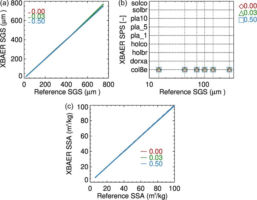
2762                                                                   L. Mei et al.: Retrieval of snow properties from SLSTR

Figure 2. Reflectance of snow layer at 0.55 and 1.6 µm calculated assuming different SPSs. Observation/illumination geometry: SZA, VZA
and RAA were set to 70, 30 and 135◦ , respectively.

weak for droxtals and aggregates of 8 columns. However, re-          requires accounting for the dependence of the phase function
flectance at 0.55 µm decreases with an increase in SGS for           on SGS.
hollow columns and plates. The weak oscillations for the re-            The main findings of the presented investigations can be
flectances at 0.55 µm can be explained by the joint impact of        formulated as follows:
oscillations in the single-scattering albedo and elements of
the scattering matrix presented in the original database. Al-           – Reflectance of a snow layer depends on both SGS and
though the reason for the oscillation in the database is un-              SPS.
clear, it is unlikely due to physical phenomena (Masanori               – Accurate simulation of snow surface reflectance re-
Saito, personal communication, 2021).                                     quires accounting for the dependence of the phase func-
   To illustrate this point, the dependence of the phase func-            tion on SGS.
tion at a 129◦ scattering angle on SGS is shown in the left
panel of Fig. 3. The phase functions (F11 element of the scat-          – Spectral channels in the visible spectral range are more
tering matrix) were extracted from the original database. Ac-             sensitive to SPS compared to SGS.
cording to the left panel of Fig. 3, the dependence of snow
surface reflectance at 0.55 µm on SGS and SPS is caused                 – Spectral channels in the near-infrared spectral range are
mainly by the phase function of ice crystals. Weak oscilla-               more sensitive to SGS compared to SPS.
tions can also be found.                                                Although the global classification of snow crystal, ice
   The above analysis shows that accurate retrieval of SGS           crystal, and solid-precipitation particles suggested in Kikuchi
requires adequate information about SPS and accounting for           et al. (2013) consists of 121 particle types, we restrict our-
the dependence of the phase function on SGS. To better il-           selves, in the retrieval algorithm, to nine shapes of ice crys-
lustrate the impacts of SGS on the ice crystal phase function,       tals, for which optical characteristics are represented in the
we calculated reflectance at 1.6 µm with different SGS val-          database (Yang et al., 2013). And these nine shapes have
ues. The right panel of Fig. 3 represents the reflectance of         been proven, especially from satellite observations, to be able
the snow layer, consisting of aggregates of 8 columns, cal-          to reproduce typical wavelength/angular features of snow re-
culated accounting for the dependence of the phase function          flectance in reality (Räisänen et al., 2015; Pirazzini et al.,
on the effective radius (black line) and assuming a constant         2015; Saito et al., 2019; Schneider et al., 2019; Pohl et al.,
phase function for three selected effective radii equal to 15,       2020b). To further illustrate that the selected dataset is able to
150 and 1150 µm (red, green and blue lines, respectively). It        reproduce the BRF of different snow types, we compared the
can be seen that the accurate simulation of snow reflection          simulated and measured BRF of fresh (Dumont et al., 2010)

The Cryosphere, 15, 2757–2780, 2021                                                      https://doi.org/10.5194/tc-15-2757-2021
L. Mei et al.: Retrieval of snow properties from SLSTR                                                                                    2763

Figure 3. Left panel: phase function at 0.55 µm for scattering angle of 129◦ , extracted from the original database (Yang et al., 2013) as a
function of effective radius. Right panel: reflectance of snow layer at 1.6 µm consisting of aggregates of 8 columns, calculated assuming that
(1) phase function depends on the effective radius (black line), (2) phase function is constant corresponding to the effective radius of 15 µm
(red line), (3) same as (2) but for effective radius of 150 µm (green line) and (4) same as (2) but for effective radius of 1150 µm (blue line).

and aged (Peltoniemi et al., 2009) snow samples. To repro-                Polarization & Anisotropy of Reflectances for Atmospheric
duce the spectral BRF by SCIATRAN, we use the setup de-                   Sciences coupled with Observations from a Lidar (PARA-
scribed above in this section and adjust the SGS for each SPS             SOL) measurements over a pure snow surface in Greenland
by minimizing the deviation between simulated and mea-                    (70.5◦ N, 47.3◦ W) on 6 July 2008 were compared with the
sured reflectance at 1.6 µm. Figure 4 shows the simulated                 SCIATRAN simulations, using droxtals, solid bullet rosettes
BRF in the principal plane at 0.55 µm of fresh and aged snow              and solid columns.
samples, as well as the respective measurements. The BRF                     According to the above analysis, we can formulate the
is defined as π I /F , where I is the reflected radiance and              general algorithm to retrieve SGS and SPS from satellite ob-
F is the incident irradiance. According to Fig. 4a, for fresh             servations. Satellite provides the wavelength-dependent TOA
snow, plates are the best shape to reproduce the measured                 reflectance. For a given SGS and SPS pair, the minimization
BRF in the vicinity of the forward scattering peak but plates             between satellite-observed TOA reflectance and theoretical
underestimate the BRF at higher viewing zenith angles in the              simulation is performed. The optimal SGS and SPS are ob-
backscattering region. Here, shapes of hollow bullet rosette,             tained when the difference between observations and simu-
hollow column and aggregate of 10 plates exhibit better po-               lations reaches the predefined criteria. The SSA is then cal-
tential to simulate the fresh-snow-layer BRF. In the case of              culated by the retrieved SGS and SPS.
aged snow, shapes of solid and hollow column, hollow bullet
rosette, and aggregate of 5 and 10 plates provide BRF val-
ues in conformity with respective measurements. However,                  4    XBAER algorithm
they slightly underestimate the BRF at high zenith angles in
                                                                          The retrieval algorithm consists of three stages. The first
the backscattering region where aggregates of 8 columns can
                                                                          stage includes the estimation of SGS using the effective Lam-
simulate the aged-snow BRF better.
                                                                          bertian surface albedo after atmospheric correction for se-
   The above analysis demonstrates that the selected database
                                                                          lected observation geometries and wavelengths. This step is
of SPS can be used successfully to reproduce measured BRF
                                                                          performed based on the path radiance representation (Mei et
of both fresh and aged snow samples. Similar results were
                                                                          al., 2017), in which the TOA reflectance can be described by
obtained by Pohl et al. (2020b). In this paper, the top-of-
                                                                          the contribution from the atmosphere and the interaction be-
atmosphere BRF at 865 nm derived from POLarization and
                                                                          tween atmosphere and surface. The inverse to derive the sur-
Directionality of the Earth’s Reflectances 3 (POLDER-3) on
                                                                          face reflectance from the satellite-observed TOA reflectance

https://doi.org/10.5194/tc-15-2757-2021                                                           The Cryosphere, 15, 2757–2780, 2021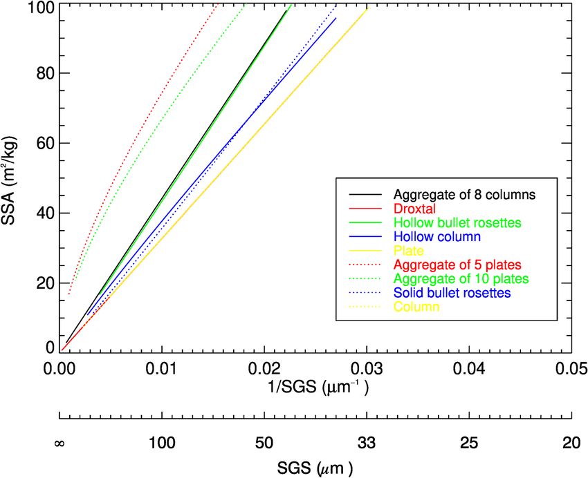
2764                                                                   L. Mei et al.: Retrieval of snow properties from SLSTR

Figure 4. The comparison of angle dependence of laboratory-measured and simulated snow reflectance: (a) fresh snow sample and (b) aged
snow sample. Symbols are measurements and lines are simulations with SCIATRAN, assuming different SPSs (see legend).

is called the atmospheric correction. And due to certain as-         constant. In our case, this results in At = 4Ap and SSA for
sumptions in the path radiance representation, the derived           convex particles such as droxtals, solid columns and plates is
surface reflectance is equivalent to the effective Lambertian        equal to 3/ρr. In the case of non-convex particles, the calcu-
surface albedo. The estimation of SGS is obtained solving the        lation of SSA requires information about total area At . Al-
following minimization problem with respect to the effective         though the database given by Yang et al. (2013) does not
radius, r, of snow crystals:                                         contain information about At , the total area of non-convex
                                                                     particles can be calculated employing the geometric param-
kAe − R s (r)k2 → min.                                       (1)     eters of ice crystal habits presented in Table 1 of Yang et al.
                                                                     (2013). Here we take a typical SPS, aggregate of 8 columns,
Here, Ae and R s (r) are two vectors whose components are
                                                                     as an example, to show the difference between SSA calcu-
the effective Lambertian surface albedo and the simulated
                                                                     lated assuming convex and non-convex particles.
snow reflectance, respectively. The dimension of these vec-
                                                                        According to Masanori Saito (personal communication,
tors is the number of wavelengths times the number of view-
                                                                     2021), the parameters L and a of the aggregate of 8 columns
ing directions.
                                                                     (see Fig. 3 in Yang et al., 2013, for details) can be obtained
   The simulation of snow reflectance (components of vec-
                                                                     by scaling with respect to the maximum dimension, D. To
tors R s (r)) was performed using the radiative transfer pack-
                                                                     find these values for different maximal dimensions, we cal-
age SCIATRAN (Rozanov et al., 2014) as described in
                                                                     culate at first the volume of the aggregate of 8 columns cor-
Sect. 3. The optical properties of nine SPSs, listed in Table 1,
                                                                     responding to parameters a and L on a relative scale as given
were used for radiative transfer calculations.
                                                                     in Table 1 of Yang et al. (2013).
   The minimization problem formulated by Eq. (1) was
solved separately for each SPS using Brent’s method (Brent,                √ 8
                                                                          3 3X
1973). The solution of the minimization problem for each             Vr =       a 2 Li                                            (4)
crystal habit is characterized by the following residual:                  2 i=1 i

1i = Ae − R s (ri∗ ) ,
                      2
                           i = 1, 2, . . ., 9,               (2)     Using the database of Yang et al. (2013), one can obtain the
                                                                     maximal dimension, Dr , corresponding to the volume, Vr . In-
where ri∗ is the solution of minimization problem given by           troducing the scaling factor, Ck = Dk /Dr , we have the semi-
Eq. (1) for the ith shape of the ice crystal particle.               width and length for the aggregate with the maximal dimen-
   The second stage is the selection of such i values (SPS)          sion Dk :
for which 1i is minimal. This completes the retrieval process
and enables the optimal SGS and SPS to be obtained.                  ai,k = ai Ck ,   Li,k = Li Ck .                              (5)
   The third stage is to calculate SSA for the retrieved SGS
                                                                     The total surface of the aggregate on a relative scale is given
and SPS. To this end, let us rewrite the SSA introduced above
                                                                     by
in the following equivalent form:
                                                                              8 √
SSA = 3/ρr · (At /4Ap ),                                     (3)     Sr = 3
                                                                              X
                                                                                  3ai2 + 2ai Li .                                 (6)
                                                                              i=1
where r is the effective radius. According to Cauchy’s sur-
face area formula (Cauchy, 1841; Tsukerman and Veomett,              Accounting for Eq. (5), we have
2016), the average area of the projections of a convex body
is equal to the surface area of the body, up to a multiplicative     S = Ck2 Sr .                                                 (7)

The Cryosphere, 15, 2757–2780, 2021                                                      https://doi.org/10.5194/tc-15-2757-2021
L. Mei et al.: Retrieval of snow properties from SLSTR                                                                                2765

                                                                             5     Impact of model parameters uncertainty

                                                                             The accuracy of any retrieval algorithm depends not only on
                                                                             measurement errors but also on the uncertainty in parameters
                                                                             which cannot be retrieved. In our case, such parameters are
                                                                             ice crystal roughness, aerosol contamination and cloud con-
                                                                             tamination. The impacts of these factors on XBAER-derived
                                                                             SGS and SPS have been investigated and will be discussed
                                                                             in this section. The TOA reflectances at selected channels
                                                                             (0.55 and 1.6 µm) and observation directions for SZA, VZA
                                                                             and RAA of 70, 30 and 135◦ for nadir and 70, 55 and 135◦
                                                                             for oblique, respectively, were calculated using the radiative
                                                                             transfer model SCIATRAN. The details of each scenario will
                                                                             be presented in the corresponding sub-section below.

                                                                             5.1    Impact of snow particle shape

Figure 5. Relationship between SGS and SSA for different SPSs.               Since the first stage of the XBAER algorithm is to estimate
For a better illustration, the realistic range of specific surface area is   the SGS assuming a given SPS, it is reasonable to investi-
limited to 100 m2 kg−1 .                                                     gate the impact of SPS on the retrieval of SGS. The TOA re-
                                                                             flectances of a snow layer at 0.55 and 1.6 µm with the above-
                                                                             given observation geometries were calculated using the fol-
Having obtained the total area, one can calculate SSA as the                 lowing settings for snow layer and atmospheric parameters:
total surface area of a material per unit of mass:
                                                                                 – Snow layer. This consists of ice crystals with SPS set
       S    Sr                                                                     to be severely roughened aggregates of 8 columns and
SSA =    =        .                                                   (8)
      ρV   ρCk Vr                                                                  maximal dimensions [100, 300, 500, 700, 1000, 2000,
                                                                                   3000, 5000] µm, which corresponds to SGS [15, 45.1,
Comparing SSA of a convex particle equal to 3/ρr with the                          75.2, 105.3, 150.4, 300.8, 451.3, 752.1] µm.
result given by Eq. (8), one can easily notice the difference in
SSA calculated from different SPSs using the same SGS. The                       – Atmosphere. This is excluded.
details of such calculations for other non-convex ice crystal
habits are given in the Appendix.                                               The simulated snow reflectances were used as components
   The relationship between SSA and SGS for different SPSs                   of vector Ae in Eq. (1). Nine SPSs from the database pre-
is presented in Fig. 5. According to Fig. 5, an almost in-                   sented in Yang et al. (2013) are used sequentially in the re-
verse linear relationship between SSA and SGS can be found.                  trieval process. The atmospheric correction is not performed
The lines, representing droxtal, plate and column, overlap,                  because the atmosphere is excluded in the forward simula-
indicating the same SSA for convex particles. For other                      tions. This enables avoiding additional errors caused by the
SPSs with the same SGS, SSA is larger compared to con-                       atmospheric correction and estimates the pure effect of SPS
vex faceted particles. SSA is restricted to the range of 0–                  on the retrieval results. Figure 6 shows the impact of the
100 m2 kg−1 in this investigation (Picard et al., 2009). For                 SPS on SGS retrieval. Different colors and line styles indi-
example, for SGS = 100 µm, the SSA is 32.7 m2 kg−1 for                       cate different ice crystals used in the retrieval process. The
convex faceted particles, whereas SSAs for aggregate of 8                    solid black line represents the retrieved SGS assuming the
columns, hollow bullet rosette, hollow column, aggregate of                  SPS in the retrieval process is the same as in forward sim-
5 plates, aggregate of 10 plates and solid bullet rosette are                ulations. This line agrees well with the 1 : 1 line, indicating
44.2, 43.4, 37.7, 74.4, 66.8 and 35.6 m2 kg−1 , respectively.                that the retrieval algorithm has been implemented technically
The relative differences range from 9 %–128 %, depending                     correctly. According to Fig. 6, one can see both underestima-
on the SPS. Taking into account the definition of SSA, one                   tion and overestimation of SGS depending on the SPS used
can derive the following relationship between SSA convex                     in retrieval. However, in most cases, an incorrect SPS leads
and non-convex particles: SSAnc = SSAc · (At /4Ap ), where                   to an underestimation of SGS. In particular, the maximal ef-
subscript c and nc denote convex and non-convex particles,                   fect can be seen when ice crystals of plate shape, rather than
respectively. The obtained results reveal that for all non-                  of the correct aggregate of 8 columns, is used (solid yellow
convex ice crystals under consideration, At /4Ap > 1 and the                 line). This result can be easily explained coming back to the
ratio At /4Ap weakly depends on the SGS.                                     right panel of Fig. 2. Indeed, one can see that the same re-
                                                                             flectance of the snow layer can be obtained using the plate
                                                                             shape, instead an aggregate-of-8-columns shape, with a sig-

https://doi.org/10.5194/tc-15-2757-2021                                                           The Cryosphere, 15, 2757–2780, 2021
2766 L. Mei et al.: Retrieval of snow properties from SLSTR
Figure 6. Impact of SPS on the retrieval of SGS. Figure 7. Impact of SGS and SPS on the retrieval of SSA. (a) SGS
errors – the black line with dots indicates the 0 difference for accu-
rate SGS for aggregate of 8 columns, and the grey area indicates the
nificantly smaller SGS. These results reveal that the SPS is an relative error in SSA introduced by a 16 % error in SGS; (b) SPS se-
important parameter affecting the accuracy of retrieved SGS. lection – different color and line styles indicate different SPSs used
in the calculation of SSA while the true SPS is set to be “plate” or
5.2 Impact of SGS and SPS on SSA other convex particles.
Since the SSA is obtained from the retrieved SGS and SPS,
an understanding of how the error in SGS and/or SPS prop- discussion with respect to uncertainty in the campaign-based
agates to the SSA will provide helpful information to under- measurement is out of the scope of this paper.
stand the retrieved SSA. Figure 7 shows the impact of SGS
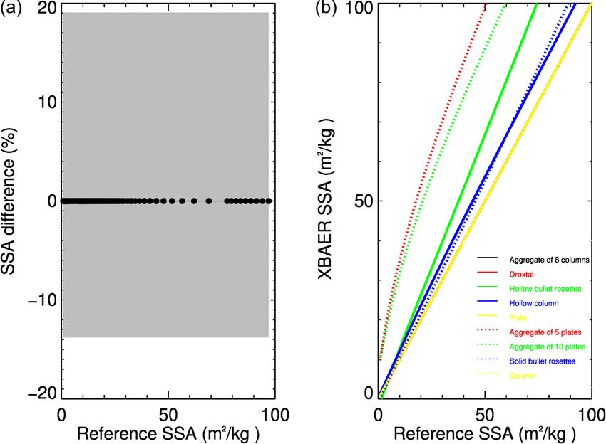
(left) and SPS (right) on XBAER-retrieved SSA. The rela- 5.3 Impact of ice crystal surface roughness
tive error in SGS, εr = (r − r 0 )/r, is propagated to the rela-
tive error in SSA as εSSA = 1 − 1/(1 − εr ), and it is indepen- Although the surface roughness of ice crystals is not too se-
dent of the reference SSA. The left panel of Fig. 7 depicts vere for snow compared to ice cloud due to basic thermody-
εSSA corresponding to ±0.16 of εr . One can see that this namics (Colbeck, 1980, 1983), the ice crystal surface rough-
results in 19 % and −13.8 % of SSA relative errors, which ness (ICSR), indicating ice crystal surface texture, may still
are presented as the upper and lower error boundaries in be important for the retrieval of snow properties from op-
the left panel of Fig. 7. The systematical error of ±16 % tical sensors such as SLSTR. The ICSR has been used as
for SGS was obtained as the maximal relative difference be- a new variable in model simulation (Järvinen et al., 2018).
tween XBAER-retrieved SGS and both in situ and aircraft- Retrieval algorithms of ice cloud parameters are frequently
measured SGS (as presented in the companion paper – Mei et based on the assumption that the ice crystal surface is smooth
al., 2021). This represents the worst case of SGS error prop- (Kokhanovsky et al., 2019). This assumption can however
agation into SSA. introduce large uncertainty in the ice cloud retrieval param-
The impact of SPS on SSA is demonstrated in the right eters and, as a consequence, lead to misunderstanding the
panel of Fig. 7. As a reference shape, we have selected in impacts of ice clouds on global climate change (Järvinen et
this case the plate, which provides the same SSA as other al., 2018). However, this issue has not yet been discussed for
convex particles. One can see that the SSA of non-convex snow. In general, ice crystal surfaces are rougher in clouds
particles overestimates the SSA of convex particles, which than in snow layers due to metamorphism processes (Col-
is in line with the results presented in Sect. 4. For instance, beck, 1980, 1983; Ulanowski et al., 2014). The investiga-
for the same SGS, the SSA for aggregate of 8 columns (non- tion of the impact of ICSR on retrieval of snow properties
convex particle) is about 3 times larger than that for doxtal provides valuable information to understand the XBAER al-
(convex particle). Since the assumption of the sphere (con- gorithm. The ICSR according to Yang et al. (2013) is de-
vex particle) is used to measure SSA in-field measures (Gal- fined similarly to the definition suggested by Cox and Munk
let et al., 2009; Nick Rutter, personal communication. 2021), (1954) for the roughness of the sea surface. A parameter σ
such as observations from SnowEx, the retrieval results of describes the degree of ICSR. The σ values 0, 0.03 and 0.5
SSA from XBAER will be systematically larger than field are for three surface roughness conditions: smooth, moderate
measurements in the case of non-convex particles even if the roughness and severe roughness. And only the above three
retrieved and measured SGSs are similar. However, a detailed values are available in the Yang et al. (2013) database. The
The Cryosphere, 15, 2757–2780, 2021 https://doi.org/10.5194/tc-15-2757-2021L. Mei et al.: Retrieval of snow properties from SLSTR 2767
Figure 8. Impact of ice crystal surface roughness (ICSR) on the Figure 9. Impact of aerosol contamination on the retrieval of SGS
retrieval of SGS (a), SPS (b) and SSA (c). Different colors indicate (a) SPS (b) and SSA (c). Different colors indicate different AOT
different ICSRs used in the retrieval. used in forward simulations. No atmospheric correction is per-
formed in the retrieval, black dash line is the 1 : 1 line.
snow layer reflectances were used as components of the vec-
tor Ae in Eq. (1) in the same way as in Sect. 5.1. low latitudes (e.g., Canadian Arctic, Tibetan Plateau) due to
Figure 8 shows the impact of ICSR on the retrieved SGS, large absolute uncertainty in the MERRA-simulated aerosols
SPS and SSA. The impact of ICSR on SGS and SSA are rel- over middle–low latitudes in wintertime. A detailed compar-
atively small for SGSs smaller than ∼ 300 µm. Ignoring the ison of how possible aerosol contamination may affect the
impact of roughness leads, in general, to a slight overestima- retrieved snow properties will be included in the companion
tion of SGS and an underestimation of SSA. The absolute er- paper (Mei et al., 2021). In the companion paper, the compar-
rors in SGS and SSA introduced by ICSR range from 0.3 %– ison between satellite-derived and campaign-measured snow
3 %, depending on SGS. Due to the inverse almost linear re- properties all over the world will be included. In order to have
lationship between SSA and SGS, as presented in Fig. 5, for a better understanding of aerosol contamination on snow
the same SPS, an overestimation of SGS leads to an under- property retrieval, the TOA reflectances were calculated at
estimation of SSA. The slight overestimation can be found if 0.55 and 1.6 µm with the above-given observation geometries
less ICSR is taken into account in retrieval because the snow using the following settings:
reflectance with the same SGS and SPS for ICSR = 0.5 is
larger than for ICSR = 0.03 due to the lower asymmetry fac- – Snow layer. This is the same as in Sect. 5.1.
tor of ice crystals with more roughened surface roughness; – Atmosphere. Aerosol type is set to be weakly absorb-
thus the same surface reflectance observed by satellite re- ing (Mei et al., 2020b) with AOTs of [0.05, 0.08, 0.11].
quires a larger SGS for the case with ICSR = 0.03 used in Other atmospheric parameters are set according to the
retrieval in contrast to ICSR = 0.5 used in the forward simu- Bremen 2D chemical transport model (B2D CTM) for
lation. However, as can be seen from the right panel of Fig. 8, April at 75◦ N (Sinnhuber et al., 2009). It is worth notic-
the XBAER algorithm still retrieves the correct SPS ignoring ing these three AOT values represent background, aver-
the impact of roughness. age and pollution conditions in the Arctic as suggested
by Mei et al. (2020a, b).
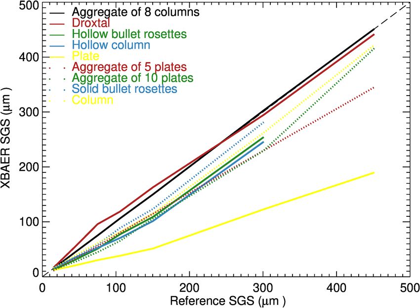
5.4 Impact of aerosol contamination
Figure 9 shows the impact of aerosol contamination on the
The impact of aerosols on the retrieval of snow properties SGS (a), SPS (b) and SSA (c) retrieval. These results are ob-
using passive remote sensing can be important because there tained by introducing a 50 % error into AOT at the step of
is limited aerosol information over the cryosphere (Mei et atmospheric correction and can be considered the worst case
al., 2013a, b, 2020a; Tomis et al., 2015) to perform an accu- for impact of aerosol contamination on retrieved SGS, SPS
rate atmospheric correction. The use of MERRA-simulated and SSA. The surface reflectances estimated after employ-
AOT, although of good data quality, will still introduce po- ing the atmospheric correction were used as components of
tential aerosol contamination into the XBAER-derived snow the vector Ae in Eq. (1). One can see that aerosol introduces
properties. The impact of aerosols on snow property retrieval systematic underestimation of retrieved SGS for the given
is much smaller over Arctic regions compared to middle– scenarios and the magnitude of underestimation increases
https://doi.org/10.5194/tc-15-2757-2021 The Cryosphere, 15, 2757–2780, 20212768 L. Mei et al.: Retrieval of snow properties from SLSTR
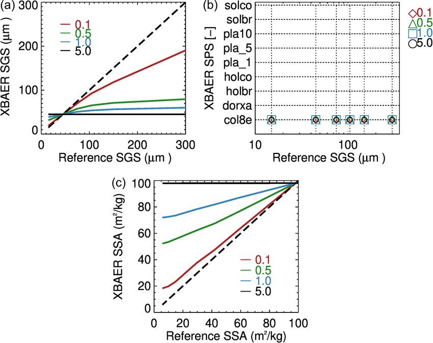
with the increase in AOT. For a typical background Arctic 6 Impact of cloud contamination
aerosol condition, with AOT = 0.05, aerosol contamination
introduces errors in SGS of less than 3 % for SGS ≤ 150 µm Any cloud-screening method, especially over the cryosphere,
and less than 7 % for 150 ≤ SGS < 300 µm. The maximal may introduce cloud contamination for the retrieval of at-
errors introduced by the aerosol contamination increase to mospheric and surface properties (Chen et al., 2014; Mei et
30 % and 37 % in the case of average and pollution condi- al., 2017; Jafariserajehlou et al., 2019). Understanding of the
tions for AOT = 0.08 and AOT = 0.11, respectively. Please cloud contamination will provide valuable information to in-
note that the AOT values in the Arctic can be even smaller terpret the retrieval results using the SLSTR instrument. To
than 0.05, for instance, AOT over Greenland. Thus, the anal- investigate the impact of cloud contamination, the following
ysis with respect to aerosol contamination is the worst case settings were used to perform the simulations of TOA re-
for a typical Arctic condition. flectance:
For the case of AOT = 0.05, SPSs have been correctly re-
– Snow layer. This is the same as in Sect. 5.1.
trieved for all SGS values, indicating that under a typical
Arctic clean condition, the impact of aerosols is not so large – Atmosphere. An aerosol-free atmosphere is used with
as to disturb SPS retrieval. In order to demonstrate the two- other parameters as in Sect. 5.4. Additionally, vertically
stage retrieval process and illustrate the impact of aerosols, homogeneous ice cloud consisting of aggregates of 8
let us focus on Fig. 10. To facilitate the presentation, we columns with an effective radius of 45 µm and optical
consider the measurement of reflectance at 1.6 µm for a sin- thickness [0.1, 0.5, 1.0, 5] is set to be at the position of
gle observation direction (30◦ ) and at 0.55 µm for the differ- [5, 6] km.
ence in reflectance at two observation angles (30 and 55◦ ).
This enables the avoiding of the minimization process given Figure 11 shows the impact of cloud contamination on
by Eq. (1) and represents the retrieval process in a simple XBAER-retrieved SGS (a), SPS (b) and SSA (c). The size of
graphic form. The left panel of Fig. 10 depicts the determina- ice crystals in ice clouds is typically smaller than snow grain
tion of an effective radius for each ice crystal form, assuming size (Kikuchi et al., 2013). Our statistical analysis of the
the correct shape is aggregate of 8 columns with an effective ice crystal effective radius over Greenland shows an average
radius of 105.4 µm. Solid and dotted lines are the surface re- value in the range of 30–50 µm, which is consistent with pre-
flectance of the snow layer consisting of ice crystals with dif- vious publications (King et al., 2013; Platnick et al., 2017).
ferent forms, and the dashed line is the measured reflectance According to Fig. 11, an overestimation of SGS can be found
after the atmospheric correction. The obtained SGSs are in for SGSs of less than 45 µm (cloud effective radius) and an
the range 40–120 µm, depending on the selected SPS, and underestimation of SGS can be found for SGSs larger than
presented in Fig. 10 by solid and dotted vertical lines. In the 45 µm. The magnitude of overestimation/underestimation in-
case of correct SPS selection (aggregate of 8 columns) the creases with the increase in cloud optical thickness (COT).
retrieved SGS is ∼ 110 µm. The right panel of Fig. 10 shows XBAER-derived SGS becomes saturated for COT larger than
the second stage of the retrieval process, namely, the selec- 0.5. Due to a limited photon penetration depth for optically
tion of an SPS for which the difference between the mea- thicker clouds (e.g., COT = 5), the XBAER algorithm re-
sured (dashed line) and simulated (solid black line) value is trieves the effective radius of ice crystals in the cloud. This
minimal. In the case under consideration the correct shape is demonstrates that theoretically, the XBAER algorithm can
selected with an effective radius of ∼ 110 µm. retrieve an ice cloud effective radius without pre-processing
For larger-AOT conditions, an inaccurate selection of SPS of cloud screening. And this can be further used as post-
occurs for all SGS cases, indicating the remaining aerosol processing to avoid cloud contamination.
information is strong enough to decouple the aerosol contri- The impact of the cloud on the retrieval of SPS is similar to
bution from the snow surface characteristic. Thus, a quality the impact of aerosols considered above. In short, the cloud
flag of SPS, associated with AOT, should be introduced into plays a larger role for larger SPSs (darker TOA) and this im-
the retrieval of real satellite data. It is interesting to see that pact increases with the increase in COT. However, cloud with
“solid bullet rosette” is the preferable SPS for very strong large COT can be much more easily detected and excluded
aerosol contamination cases. This is due to the similar scat- by the cloud-screening algorithm (e.g., for the cases with
tering properties (shape) of ice crystals and weakly absorb- COT > 0.5). SPSs are correctly picked up due to the same
ing aerosols, defined in forward simulation. The impact of SPS used for both the snow layer and the cloud layer. Sim-
aerosol contamination, for typical Arctic conditions, intro- ilarly to the impact of aerosol, the underestimation of SGS
duces a less-than-5 % error into SSA. However, for large introduced by the cloud leads to an overestimation of SSA
aerosol contamination, the around 30 % underestimation in (Fig. 11c). The increase in COT results in saturation of the
SGS linearly introduced about 25 % overestimation in SSA, ice cloud SSA, with a value of 100 m2 kg−1 in the case of
which agrees with the analysis as presented in Fig. 7. aggregates of 8 columns.
The Cryosphere, 15, 2757–2780, 2021 https://doi.org/10.5194/tc-15-2757-2021L. Mei et al.: Retrieval of snow properties from SLSTR 2769
Figure 10. Schematic representation of two stages of the retrieval process. (a) Determination of effective radius for each ice crystal form.
(b) Selection of optimal SGS–SPS pair.
ment spectral response function (SRF), and the other one is
the representativeness of the snow scenario for reality.
7.1 Impact of instrument spectral response function
– Snow layer. This is the same as in Sect. 5.1.
– Atmosphere. An aerosol-free atmosphere is used with
other parameters as in Sect. 5.4.
The forward simulations are performed with and without
the impact of the spectral response function (SRF). The SRFs
for SLSTR at 0.55 and 1.6 µm are shown in Fig. 12. The re-
trieval is then performed ignoring the SRF. Figure 13 shows
the impact of SRF on the retrieval of SGS, SPS, and SSA.
For forward simulations without taking the SRF into account
(labeled as No in Fig. 13), SGS, SPS and SSA are well re-
Figure 11. Impact of cloud contamination on the retrieval of
ceived as expected. And this agrees with Fig. 6. However,
SGS (a), SPS (b) and SSA (c). Different colors indicate different ignoring the impact of the SRF introduces about 7 % uncer-
COTs in forward simulations; dashed black line is the 1 : 1 line. tainties into the simulated surface reflectance, and this causes
about a 5 %–7 % error in both SGS (overestimation) and SSA
(underestimation). Taking the SRF into account leads to a
smaller surface reflectance at 1.6 µm due to potential gas ab-
7 Impact of other factors occurring in reality
sorption at this wavelength and thus introduces an overesti-
mation for SGS. However, due to a significantly smaller im-
The above theoretical investigations include all possible im-
pact at 0.55 µm, the SRF does not play a significant role in
portant factors affecting the accuracy of the XBAER algo-
the retrieval of SPS.
rithm. However, when applying the XBAER algorithm to the
SLSTR instrument for real scenarios, two additional factors
need to be considered as well: one is the impact of the instru-
https://doi.org/10.5194/tc-15-2757-2021 The Cryosphere, 15, 2757–2780, 20212770 L. Mei et al.: Retrieval of snow properties from SLSTR
where k and v are the shape and scale parameters, the nor-
malization factor C is defined as
−1
D
Zmax
C= (D/v)k−1 e−D/v dD , (11)
Dmin
and Dmin and Dmax describe the minimal and maximum par-
ticle sizes in the distribution.
In order to introduce the vertical inhomogeneity, we use
the measurement of snow density and equivalent optical
diameter vertical profiles conducted during the SnowEx17
campaign. Accounting for the fact that the equivalent optical
diameter cannot be directly used to define parameters of the
gamma distribution, we use the vertical profile as a shape of
the mode (most frequent value in a dataset); i.e.,
Figure 12. Spectral response function of (a) 0.55 and (b) 1.6 µm of
De (z)
the SLSTR instrument. D0 (z) = D0 (ztop ), (12)
De (ztop )
where De (z) is the measured vertical profile of equivalent op-
tical diameter and D0 (z) is the vertical profile of the mode.
The mode near the top of the snow layer, D0 (ztop ), is as-
sumed to be equal to 400 µm according to the measurement
data reproduced by Saito et al. (2019) in their Fig. A1.
Taking into account the analytical expression of the mode
via shape and scale parameters,
D0 = (k − 1)v, (13)
and the relationship between shape and scale parameters de-
rived by Saito et al. (2019),
k = 11.38v −0.167 − 2, (14)
we can estimate parameters k and v of the gamma distribu-
tion corresponding to D0 (z) given by Eq. (12).
Figure 13. Impact of SRF on the retrieval of SGS (a), SPS (b) and
The snow grain habit mixture (SGHM) model is used ac-
SSA (c). Different colors indicate retrieval results without (No) and cording to Saito et al. (2019). In particular, the particle habits
with (Yes) the SRF in forward simulations; dashed black line is the include droxtal, solid hexagonal column and solid bullet
1 : 1 line. rosette. The habit fraction, fh (D), as a function of the maxi-
mal dimension of the SGHM model is presented in Fig. 15b.
The habit fraction is defined so that, for each D,
7.2 Impact of snow inhomogeneities
3
X
In this section, a realistic model of the snow layer is repre- fh (D) = 1. (15)
h=1
sented by a vertically inhomogeneous, polydisperse ice crys-
tal habit mixture. Following Saito et al. (2019), the gamma The selected SGHM model enables us to derive the total vol-
distribution with respect to the maximal dimension will be ume of ice per unit volume of air as
used to describe polydisperse properties:
Dmax
X3 Z
n(D) = N G(D). (9) Vt = N Vh (D)fh (D)G(D) dD
(16)
h=1
Dmin
Here, N is the number of ice particles per unit volume and
G(D) is the gamma distribution function; i.e., and ice water content (IWC)
G(D) = C(D/v)k−1 e−D/v , (10) IWC = Vt ρice , (17)
The Cryosphere, 15, 2757–2780, 2021 https://doi.org/10.5194/tc-15-2757-2021You can also read