Reply on Referee Comment RC1 on acp-2021-52 - Recent

Reply on Referee Comment RC1 on acp-2021-52
In the following the comments of the referee are presented (in black) alongside with our replies (in blue)
and changes made to the manuscript (in red).
General statement: The manuscript presents original and valuable experimental results accompanied by
global model calculations. Furthermore, it is generally well written and presented. I suggest acceptance
of the manuscript for publication, but I have a few minor comments to be considered before the final
acceptance.
Dear reviewer, thank you very much for reviewing our manuscript and for the insightful comments. Below
we provide detailed responses to your comments.

Comment 1: line 35: The wording “NOx is a toxic gas” sounds rather odd as NOx is not a single gas. To
avoid misunderstandings the wording could be revised.
We have revised the sentence. It now says in line 35: Both NO and NO2 are toxic gases which degrade
surface air quality and regulate the abundance of secondary tropospheric oxidants.

Comment 2: line 41: The sentence needs revision.
We have revised the sentence. It now says: The U.S. Clean Air Act identified ozone as a criteria air
pollutant in the 1970s (Jaffe et al., 2018).

Comment 3: line 84: You may also add some earlier references on NOx-VOC sensitivity of ozone
production by Sillman.
We have added the already cited study of Sillman et al. “Photochemistry of ozone formation in Atlanta,
GA – models and measurements” (1995) as a reference and another study by Sillman et al., “O3-NOx-
VOC sensitivity and NOx-VOC indicators in Paris: Results from models and Atmospheric Pollution Over
the Paris Area (ESQUIF) measurements” to the list of references and as a reference to line 84: (Sillman
et al., 1995; Sillman et al., 2003; Duncan et al., 2010, Nussbaumer and Cohen, 2020, Tadic et al., 2020).

Comment 4: lines 85-86: Please add a reference for the lifetime of NOx.
We have added a reference to lines 85-86 (Beirle et al., 2010).

Comment 5: There are a number of NOPR studies based on in situ HOx or ROx measurements by
aircraft or at high altitudes stations which could be considered, e.g. Cantrell et al., 1996, Zanis et al.,
2000, Cantrell et al., (2003a), Ren et al., (2008) Olson et al., (2012).
We have added Zanis et al. (2000a; The Role of In Situ Photochemistry in the Control of Ozone during
Spring at the Jungfraujoch (3,580 m asl) – Comparison of Model Results with Measurements;
https://doi.org/10.1023/A:1006349926926) and Cantrell et al. (2003; Peroxy radical behavior during the
Transport and Chemical Evolution over the Pacific (TRACE-P) campaign as measured aboard the NASA
P-3B aircraft; https://doi.org/10.1029/2003JD003674) to the list of references.
We have added the following sentence to the manuscript in line 367 (referencing Zanis et al., 2000a):
The negative net ozone tendencies observed between 3 and 5 km altitude for the tropical troposphere
stand in opposition to positive net ozone tendencies of about 0.1 ppbv h-1 (Zanis et al., 2000a) and
balance in net ozone tendencies (NOPR ≈ 0) (HOOVER campaign over Europe; Bozem et al., 2017)
deduced from previous measurements at similar altitudes at mid-latitudes.

 1

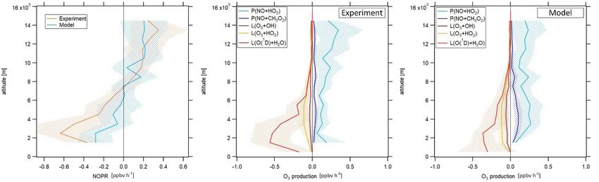
We have added the following sentence to the manuscript in line 449 (referencing Cantrell et al., 2003):
Especially the NO compensation mixing ratio (for which ozone production equals ozone loss) reproduces
results from previous studies remarkably well. Cantrell et al. (2003) report NO compensation mixing
ratios between 10 and 30 pptv over the Pacific, depending on whether modelled or measured HO 2 and
RO2 is used. A study conducted by Zanis et al. (2000b) for the Swiss Alps also reports balance in ozone
production for similar NO compensation mixing ratios. Note that this second amendment addresses
Comment 17 of our reply. The respective reference (Zanis et al., 2000b) has been added to the list of
references.
Comment 6: line 211: Should rather be “is practically one or unit” instead of unity.
We have revised line 211 accordingly.

Comment 7: line 211: Should be Tadic et al. (2017).
We have revised the passage accordingly.

Comment 8: line 235: You may also add some earlier references for the calculation of net ozone
production (e.g. Lin et al., 1986).
We have added the suggested reference to the list of references and to line 235/236. However it should
be Lin et al., 1988 (https://doi.org/10.1029/JD093iD12p15879) instead of 1986. We have further added
Cantrell et al. (2003) as a reference for this sentence.

Comment 9: line 242-243: You may add a reference for the selection of the 100 ppbv criterion for
stratospheric ozone. For example, see Prather et al., 2011. Other model intercomparison studies
generally utilized a chemical tropopause defined at the 150 ppbv.
We have added Prather et al. (2011) to the list of references. Line 242ff now says (the underlined
passage is new): Data are filtered for stratospheric influence by removing all data points for which
concurrent O3 is larger than 100 ppbv; a conservative criterion which has been discussed by Prather et
al. (2011).

Comment 10: lines 251-253: The attribution of high NOx above 12 km to lightning NOx rather than NOx
rich stratospheric air is rather speculative, unless if there are some indications from the model results of
references for that. Mind also the simultaneous relatively smooth increase of both NO and O3 (as you
also mention in page 10) which may point influence of stratospheric air.
Our argumentation is based the fact that the tropopause is located at about 16-18 km altitude at the
ITCZ, which is still about 3-5 km above typical (highest) cruising altitudes of 12 – 14 km during the
campaign. Second, although both NO and O3 show a slight increase above 12 km, the vertical CO profile
shows only a slight decrease in average mixing ratios from about 100 ppbv around 12 km altitude to 80
ppbv around 15 km altitude which is statistically insignificant within ±1 standard deviation of the vertical
average CO mixing ratio. Assuming that stratospheric influence did play a (more) dominant role in terms
of high NOx, the decrease in CO should be stronger than observed.
Also we have created two additional figures (added at the end of this reply) showing 2-D
latitudinal/altitudinal distributions of measured, tropospheric NO and O3 during the campaign. Especially
the latitudinal/altitudinal NO distribution shows rather local enhancements at the latitudinal range of the
ITCZ than intrusion from the stratosphere at the subtropical jet streams.
We have further added these two figures discussed here to the supplement (as supplement Figure S5
and Figure S6) and redefined the numbering of the following supplement Figures accordingly. A short

 2

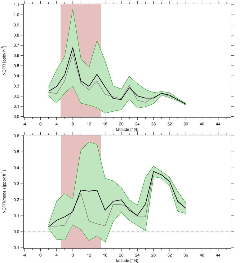
passage has been added to the manuscript in line 343: Furthermore, supplementary Figures S5 and S6
show 2-D latitudinal-altitudinal distributions of measured, tropospheric NO and O3, respectively.

Comment 11: line 264: At around 6 km it seems that there is an ozone layer of possible stratospheric
origin. You may check this with relevant model diagnostics (e.g. specific humidity, potential vorticity or
O3S if it is available from the simulation).
There is generally a lower data coverage for altitudes in the free and middle troposphere (between 4 and
10 km). The increase in modelled O3 at 6 km altitude arises from a few data points with increased mixing
ratios at this altitude. A vertical profile of modelled humidity does not reproduce stratospheric influence.

Comment 12: lines 280-281: This does not necessarily mean that you totally exclude the influence of
mixing with air of stratospheric origin.
No, we do not exclude mixing with air of stratospheric origin. To clearify this, we have added a short
notice after the respective sentence in line 281f (underlined passage is new): We again remove
stratospheric measurement data by only considering those for which O3 was below 100 ppbv. Note that
this does not necessarily exclude influence of mixing with air of stratospheric origin.

Comment 13: line 308: “…is shown..” should be deleted.
Thanks for noticing. We have removed “is shown” from the sentence.

Comment 14: line 368: Although the effect of humidity can be implied from factor of Eq. 4 maybe it is
also interesting adding in the supplementary material the observed and simulated specific humidity
values.
We agree that is makes sense to add a comparison of the vertical profiles of observed and simulated
humidity. We have added the following underlined sentence in line 349: We provide a vertical profile of
 calculated based on Eq. 4, for which we obtain good agreement between measurements and
simulations, for which we refer to the left graph of Figure S7 in the supplement. Supplementary Figure
S7 also provides a comparison of vertical profiles of measured and simulated H2O mixing ratios. The
respective comparison of measured and modelled H2O mixing ratios has been added to supplement
Figure S7 (which already shows the intercomparison of the vertical profile of and (O1D)). The revised
Figure S7 (updated in the supplement) is included at the end of our reply.

Comment 15: line 379: Should rather be: “… is from a factor of 2-3 (below 3 km altitude) to a factor of
10 (above 12 km altitude) stronger …”
We have applied the suggested change.

Comment 16: Figure 7 is interesting showing the NO dependence of NORP as well as the ozone
compensation point (the NO level at which NORP is roughly zero). One possibly limitation is the fact that
the aggregated bins correspond to different atmospheric layers with different atmospheric characteristics
which can possibly induce the spiky signal in the figure.
We agree that the spiky signature in the profile could be due to the variety of different air masses
measured during the campaign and corresponding to a certain bin. We have added the following
sentence to the passage below the figure (line 453ff): Note that one possible limitation of this figure
arises from the fact that the data aggregated in the respective NO mixing ratio bins stem from different
atmospheric layers and origins, which causes the spiky signature of the profile for both measurement
and model.
 3

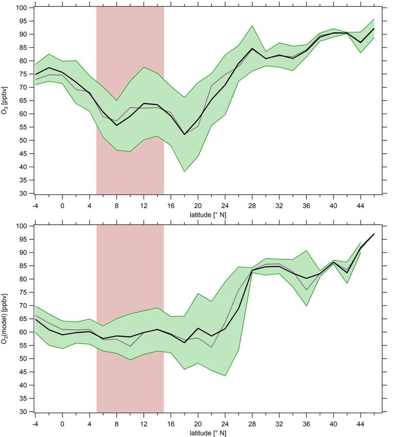
Comment 17: line 441: You may also take into consideration the ozone compensation point which was
derived in previous studies in the free troposphere and which agrees well with these values (see e.q.
Zanis et al., JGR, 2000)
Zanis, P., Monks, P. S., Schuepbach, E., Carpenter, L. J., Green, T. J., Mills, G. P., Bauguitte, S., and
Penkett, S. A.: In situ ozone production under free tropospheric conditions during FREETEX ’98 in the
Swiss Alps, J. Geophys. Res., 105, D19, https://doi.org/10.1029/2000JD900229, 2000b has been added
to the list of references. Comment 17 is being addressed within the answer to comment 7.

Figure S5: Latitudinal/altitudinal distribution of measured, tropospheric NO obtained during the campaign. The data have been
aggregated and averaged over a grid width of 2 degree latitude and 1 km altitude.

 4

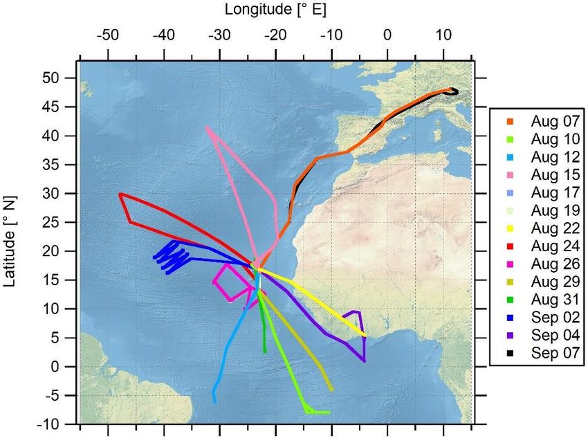
Figure S6: Latitudinal/altitudinal distribution of measured, tropospheric O3 obtained during the campaign. The data have been
aggregated and averaged over a grid width of 2 degree latitude and 1 km altitude.

Figure S7: Vertical, tropospheric profile of calculated based on measured and simulated data during CAFE-Africa (left graph).
Vertical, tropospheric profile of H2O mixing ratios calculated based on measured and simulated data during CAFE-Africa (middle
graph). Vertical, tropospheric profile of ( ) (measured and simulated) obtained during CAFE-Africa (right graph). The orange
and blue traces represent measured and simulated results, respectively.

 5

6

Reply on Referee Comment RC2 on acp-2021-52
In the following the comments of the referee are presented (in black) alongside with our replies (in blue) and
changes made to the manuscript (in red).
General description: The authors use aircraft observations of ozone and NO to estimate net ozone
production rates in the upper troposphere over the Atlantic Ocean and West Africa. They determine that
ozone production is NOx-limited. My recommendation is substantial changes to the manuscript before
this should be considered for publication in ACP. These are detailed below.
Dear reviewer, thank you very much for reviewing our manuscript and for the insightful comments. Below
we provide detailed responses to your comments.

General comments: The introduction does not provide the reader with context for what’s known about
the region and the time period sampled. The introduction details well-established ozone chemistry, rather
than referring to prior publications that focus on ozone chemistry in the region. These include, but are
not be limited to, publications that make use of observations from previous and ongoing flight campaigns
in West Africa and over the Atlantic (AMMA, DACCIWA, MOZAIC, IAGOS, CARIBIC, ATom). URLs to
some relevant publications are provided in the References section of this review. An introduction specific
to the target region would clarify whether the finding in this study is in dispute, known already, or contrary
to what’s been found before.
Similarly, the results section should be compared to results published in the literature from previously
published research.
We agree that it makes sense to provide the reader with information on ozone chemistry in the region
by including observations from previous and ongoing flight campaigns. We have added a new paragraph
to line 101ff (prior to the sentence “In the present study we characterize the distribution of NO and …):
A number of previous studies have performed measurements in the region of interest, the troposphere
over the Atlantic Ocean and the West Africa (Lelieveld et al., 2004; Aghedo et al., 2007; Saunois et al.,
2009; Real et al., 2010; Bourgeois et al., 2020). Lelieveld et al. (2004) indicated that positive ozone
trends in the marine boundary layer over the Atlantic are likely caused by an increase in anthropogenic
emissions of nitrogen oxides. Aghedo et al. (2007) showed that lightning acts as a major source of
tropospheric NOx, leading to a significant increase in middle and upper tropospheric ozone over the
African continent. Saunois et al. (2009) described results from airborne measurements in the region
during the AMMA project. Deploying a two-dimensional model for further analysis, Saunois et al.
determined positive trends in photochemical net ozone production in the boundary layer over West
Africa. There are also results from the ATom airborne mission, which measured vertical profiles of O 3 in
the troposphere over the Atlantic Ocean (Bourgeois et al., 2020), which we will use to validate the results
presented here. Real et al. (2010) investigated downwind O3 production in pollution plumes in the mid
and upper troposphere and determined mean net ozone production rates of 2.6 ppbv/day over a period
of 10 days. However, studies reporting on vertical profiles and spatial distributions of nitric oxide, ozone
and net ozone production rates as part of one coherent measurement project in the troposphere over
the West African continent and the Atlantic Ocean are absent.

We added the here mentioned five studies to the list of references:

 7

Aghedo, A. M., Schultz, M. G., and Rast, S.: The influence of African air pollution on regional and global
tropospheric ozone, Atmos. Chem. Phys., 7, 1193-1212, https://doi.org/ 10.5194/acp-7-1193-2007,
2007.

Bourgeois, I., Peischl, J., Thompson, C. R., Aikin, K. C., Campos, T., Clark, H., Commane, R., Daube,
B., Diskin, G. W., Elkins, J. W., Gao, R.-S., Gaudel, A., Hintsa, E. J., Johnson, B. J., Kivi, R., McKain,
K., Moore, F. L., Parrish, D. D., Querel, R., Ray, E., Sánchez, R., Sweeney, C., Tarasick, D. W.,
Thompson, A. M., Thouret, V., Witte, J. C., Wofsy, S. C., and Ryerson, T. B.: Global-scale distribution of
ozone in the remote troposphere from the ATom and HIPPO airborne field missions, Atmos. Chem.
Phys., 20, 10611–10635, https://doi.org/10.5194/acp-20-10611-2020, 2020.

Lelieveld, J., van Aardenne, J., Fischer, H., de Reus, M., Williams, J., and Winkler, P.: Increasing Ozone
over the Atlantic Ocean, Science, 304, Issue 5676, 1483-1487, https://doi.org/10.1126/science.1096777,
2004.

Real, E., Orlandi, E., Law, K. S., Fierli, F., Josset, D., Cairo, F., Schlager, H., Borrmann, S., Kunkel, D.,
Volk, C. M., McQuaid, J. B., Stewart, D. J., Lee, J., Lewis, A. C., Hopkins, J. R., Ravegnani, F., Ulanovski,
A., and Liousse, C.: Cross-hemispheric transport of central African biomass burning pollutants:
implications for downwind ozone production, Atmos. Chem. Phys., 10, 3027–3046,
https://doi.org/10.5194/acp-10-3027-2010, 2010.

Saunois, M., Reeves, C. E., Mari, C. H., Murphy, J. G., Stewart, D. J., Mills, G. P., Oram, D. E., and
Purvis, R. M.: Factors controlling the distribution of ozone in the West African lower troposphere during
the AMMA (African Monsoon Multidisciplinary Analysis) wet season campaign, Atmos. Chem. Phys., 9,
6135-6155, https://doi.org/10.5194/acp-9-6135-2009, 2009.

A discussion of the O3 vertical profile with respect to results from the ATom mission has been included
in the manuscript in line 300ff:
O3 profiles observed in this study are in good agreement with results from the ATom mission (Bourgeois
et al., 2020). For the June-August season, Bourgeois et al. show that in the tropical troposphere O3
increased with altitude to 50 ppbv at 5-6 km whereas above 9 km O3 varied from 40 to 80 ppbv,
supporting the results presented here (see Figures 9 and 10 in Bourgeois et al., 2020).

Another section has been added to discuss the relevance of photochemical ozone production derived in
this study in line 437:
Our results add to the understanding of photochemical net ozone production in the upper troposphere of
the region. Using a photochemical trajectory model initiated by in situ measurements, Real et al. (2010)
derived photochemical net ozone production rates of 2.6 ppbv/day over a period of 10 days downwind
of West Africa. Our study supports the findings by Real et al. (2010) by underlining that photochemical
ozone production in the upper troposphere over the tropics is positive at about 0.2-0.4 ppbv h-1, which
supports the concept of significant photochemical ozone production in the upper troposphere of the
region. Note that during CAFE-Africa, measurements at low altitudes were generally performed over the
Atlantic Ocean. Hence we cannot compare to previous results from Saunois et al. (2009) reporting ozone
production ranging from 0.25 to 0.75 ppbv h-1 in the continental boundary layer over West Africa (2009).

 8

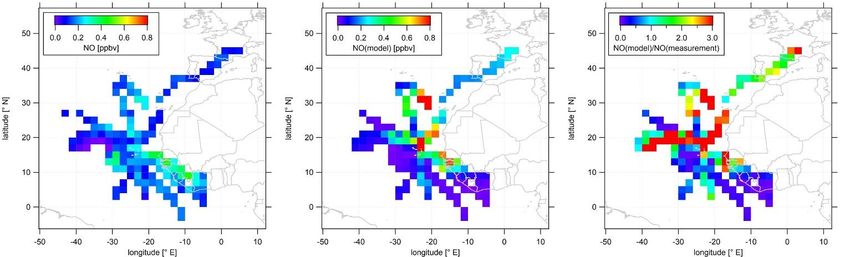
The measurement techniques the researchers use are established techniques, so instead dedicate the
methods section to describing the aspects of these that are unique and relevant to your study.
We consider the section describing the measurement methods and techniques to be essential to the
study. We have added a short sentence in line 197 emphasizing the applicability of the instrumental set
up for observations on an airborne platform:
All instruments deployed on the aircraft have been developed to meet the high standards of airborne
measurements in terms of operability, accuracy and sensitivity.

Avoid unfamiliar and unnecessary acronyms when there are mathematical symbols or familiar letters
that would be easier for the reader to follow. NOPR, RMU, and TMU are not universally familiar. For
NOPR, for example, consider rather using P(O3)net. P(O3)gross could then be used to distinguish the
two. Many acronyms in the paragraph starting on line 111 seem unnecessary and make it a challenge
to read.
We agree that it makes sense to unify “total measurement uncertainty” (TMU) and “relative measurement
uncertainty” (RMU), which describe in principle the same phenomenon. We have therefore replaced
“relative measurement uncertainty”/”RMU” in Table 1 and in the caption of Table 1 by “total measurement
uncertainty”/”TMU”.
However, in terms of the acronym NOPR we have to state that the acronym/symbol for net ozone
production rate” is not unified in the community. Previous studies (Thornton et al., 2002) used the
acrnonym “ (O3 )” as the gross rate of O3 production, which is equivalent to what is given in our study.
Also Real et al. (2010, https://doi.org/10.5194/acp-10-3027-2010) abbreviated “net ozone production” by
“NPO3”, similar to the acronym “NOPR” mentioned in our study. Last but not least, “NOPR” has already
been established in previous studies (Bozem et al., 2017; Tadic et al., 2020). We would like stay with
the used acronym “NOPR”.
Nevertheless to make it easier to follow the manuscript, we have added short notices in line 231: Note
that other studies use P(O3)gross as an acronym for P(O3) in Eq. 2.
… and in line 238:
Note that other studies use P(O3)net as an acronym for NOPR in Eq. 6.

Comment 1: Line 118: How does the flight ceiling compare to the tropopause height during the flight
campaign?
The tropopause is located at about 16-18 km altitude at the ITCZ, which is 3-5 km above the flight ceiling.
At higher latitudes (~ 30° N), the tropopause is located at about 13-15 km.

Comment 2: Figure 1 caption: Provide dates instead of flight numbers. The former are more meaningful.
We have replaced the flight numbers by flight dates. A revised version of Figure 1 (with revised caption)
can be found at the end of this document. We have revised lines 128ff in the manuscript (underlined
words are new) to facilitate the attribution of flight dates to flight numbers: For the analysis of the MFs,
we consecutively numerate each MF. We start with MF03 on August 07, 2018 for the ferry flight from
Oberpfaffenhofen (Germany, Deutsches Zentrum für Luft- und Raumfahrt) to Sal (Cape Verde Islands)
and ending with MF16 on September 07, 2018 for the back ferry flight from Sal to Oberpfaffenhofen.

Comment 3: What does the model simulate? Global?
Yes, EMAC is a global model. We have clarified this at the beginning of chapter 2.4 by adding the
attribute “global” to the description of EMAC (underlined word is new): EMAC is a 3-D global general

 9

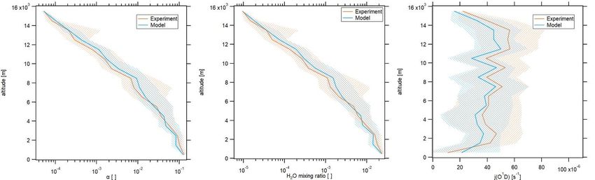
circulation, atmospheric chemistry-climate model, which has been used and described in a number of
previous studies (Roeckner et al., 2006; Jöckel et al., 2016; Sander et al., 2019; Tadic et al., 2020).

Comment 4: Are soil NOx emissions in the model? If so, give the name and reference of the inventory.
If not, would this contribute to the model-measurement discrepancy in NO in the lower troposphere?
NOx soil emissions are included in the model. However, there is no inventory itself in the model as NOx
soil emissions are calculated online by an algorithm described by Yienger and Levy II (Yienger and Levy
II, 1995; Kerkweg et al., 2006). Based on the Yienger and Levy II algorithm, Pozzer et al. have
determined a yearly emission of NOx at 6.77 to 7 TgN/yr (see supplement of Pozzer et al., 2007). Weng
et al. found that averaged over the last 37 years, global total soil NOx emissions amount to 9.5 TgN/yr
(2020), which means that NOx soil emission in the EMAC model might be on the lower end of the most
recent estimates. We have added the following sentence to the description of the model in line 216: The
NOx soil biogenic emission flux is calculated based on a semi-empirical emission algorithm
implementation by Yienger and Levy II (1995; Kerkweg et al., 2006).
Yienger and Levy II (1995) has been added to references of the manuscript. Kerkweg et al. is already
cited in the manuscript.

Yienger, J. and Levy II, H.: Empirical model of global soil-biogenic NOx emissions, J. Geophys. Res.,
100, 11 447–11 464, https://doi.org/10.1029/95JD00370, 1995.

Pozzer et al.: Simulating organic species with the global atmospheric chemistry general circulation model
ECHAM5/MESSy1: a comparison of model results with observations, Atmos. Chem. Phys., 7, 2527–
2550, 2007.

Weng et al.: Global high-resolution emissions of soil NOx, sea salt aerosols, and biogenic volatile organic
compounds, Sci Data, 7, 148 (2020).

Comment 5: Line 198: What is “tg”? Do you mean “Tg”?
Yes, we mean “Tg”. We have revised the unit accordingly (now line 214)

Comment 6: Line 211: Format of the in-text citation of Tadic et al. is incorrect.
We have revised the passage accordingly.

Comment 7: Line 213: What does “Therewith” mean? Is it necessary?
We agree that “therewith” is redundant. We have removed “therewith” from the sentence.

Comment 8: Line 217-221: This is a very lengthy sentence that makes for challenging reading.
We agree that it makes sense to rewrite this sentence. We have also clarified the acronym PSS in line
219 (which addresses comment 9). Line 236ff now say: We further assume photostationary steady state
(PSS) for the probed air masses. As the typical time to acquire PSS during CAFE-Africa varied between
40 s at 2 km altitude and about 70-80 s at 15 km altitude (Mannschreck et al., 2004; Tadic et al., 2020),
we can calculate the concentration of CH3O2 by the equation derived by Bozem et al. (2017).

Comment 9: Line 219: Tell the reader what “PSS” is.
See answer to comment 8.

 10

Comment 10: Lines 225-226: The dominant loss pathway for HCHO leading to the formation of HO2 is
photolysis. If this loss pathway is also taken into account, is HO2 production from HCHO still negligible?
In the manuscript we have conservatively estimated ambient HCHO mixing ratios at 100 pptv, which
represents an upper limit for HCHO and is most likely a factor of 2 too high. Taking into account the
photolysis of HCHO (being an additional pathway of HO2 production) results in HO2 production from the
reaction of CO with OH being on average a factor of 5 larger than the sum of HO2 production from the
sum of the reaction of H2 with OH, the reaction of HCHO with OH and photolysis of HCHO. In
combination with the fact that 100 pptv already represents an upper limit for HCHO, we still can assume
that the reaction of CO with OH dominates HO2 production during most of the campaign time to estimate
CH3O2. Nevertheless, we have incorporated this new finding into the manuscript in line 241ff: Note that
the reaction of CO with OH represents the dominant term in HO2 production during CAFE-Africa.
Assuming mixing ratios of 500 ppbv and 100 pptv for H2 and HCHO, respectively, we find that HO2
production rate from the reaction of OH with CO is on average 5 times greater than the sum of the HO2
production rates from photolysis of HCHO and the reactions of HCHO and H2 with OH during CAFE-
Africa. Note that the assumed mixing ratio of 100 pptv represents a rather conservative upper estimate
for HCHO in the upper troposphere.

Comment 11: Equation (6): Is the righthand side of this equation just “P(O3)gross – L(O3)”? If so,
consider rewriting it to this so that it is clearer that this relates to what’s given in equations (2) and (5).
Yes, the righthand side of this equation is just “P(O3)gross – L(O3)”. Equation 6 now reads as:
 NOPR = (O3 ) − (O3 ) =
 [NO] ⋅ ( NO+HO2 [HO2 ] + NO+CH3 O2 [CH3 O2 ]) − [O3 ] ⋅ (α ⋅ (O1 D) + OH+O3 [OH] + HO2 +O3 [HO2 ])

Comment 12: Lines 231: It’s not clear whether the quoted values are calculated in this work or are from
a previous study. Rewrite for clarity.
These values represent results from a previous study (Bozem et al., 2017). We have clarified this by
revising line 251: In the troposphere, ranges from about 15 % in the PBL to 1 % in the upper
troposphere, where absolute humidity is very low (Bozem et al., 2017).

Comment 13: Figure 2: Considering the simulated NO variability extends into the negative, provide the
min and max values of the modelled and observed NO.
The simulated NO variability extends into the negative due to the large variability of NO data at highest
altitudes. Note that the model itself does not yield any negative data at all. However having a few
simulated data points with large NO mixing ratios results in a relatively large standard deviation of the
respective average and, consequently, in the variability (± 1 standard deviation) being negative above
12 km altitude. The min and max mixing ratios of modelled NO are zero and 2.13 ppbv, respectively. The
mix and max mixing ratios of observed NO are zero and 0.95 ppbv. This finding has been incorporated
into the study in line 284: The minimum and maximum mixing ratios of modelled NO are zero and 2.13
ppbv, respectively. The minimum and maximum mixing ratios of observed NO are zero and 0.95 ppbv,
respectively.

Comment 14: Lines 252-253: Why would there be influence from the stratosphere if this has been
removed using an ozone concentration threshold?

 11

The ozone mixing ratio threshold of 100 ppbv only removes measurements obtained directly in the
stratosphere where O3 significantly exceeds 100 ppbv. However, this threshold does not remove all
periods with stratospheric influence. Take for instance an (upper) tropospheric air mass with intrinsically
low O3. Influence from the stratosphere could result in an increase in O 3 which however would not
necessarily result in O3 mixing ratios larger than 100 ppbv.

Comment 15: Line 309: Avoid subjective words like “interestingly”.
We have removed “interestingly” from this sentence.

Comment 16: Line 433: Change “Please note that there …” to “There …”.
We have revised line 474 accordingly. It now says: Please note that There is only limited data coverage
for measured NO above 0.325 ppbv and for simulated NO above 0.15 ppbv. See supplementary table
ST3 for the number of data points in each NO mixing ratio bin.
The second sentence of this amendment already addresses comment 18 (to add the number of data
points in each NO concentration bin.).

Comment 17: Line 432: Was there any doubt or contention that the upper troposphere is NOx-limited
over this region?
There was no doubt or contention that the upper troposphere might or might not be NO x-limited. This is
a fundamental finding, which arises from the dependency of net ozone production on NO (presented in
Figure 7), which has, as far as we know, not been presented before for the upper troposphere over the
Atlantic Ocean and West Africa.

Comment 18: Give the number of data points in each NO concentration bin.
The number of data points in each NO concentration bin are given in the following table, which has been
added to the supplements of this study. We have further revised sentence in Line 474ff: There is only
limited data coverage for measured NO above 0.325 ppbv and for simulated NO above 0.15 ppbv. See
supplementary table ST3 for the number of data points in each NO mixing ratio bin.

Table ST3: Number of data points in each NO mixing ratio bin. Note that the data coverage of the simulation is larger
than that of the measurement due to gaps in the observational data.
 NO mixing ratio bin measurement simulation
 0 pptv ≤ NO < 25 pptv 140 226
 25 pptv ≤ NO < 50 pptv 54 70
 50 pptv ≤ NO < 75 pptv 36 40
 75 pptv ≤ NO < 100 pptv 23 60
 100 pptv ≤ NO < 125 pptv 50 38
 125 pptv ≤ NO < 150 pptv 44 24
 150 pptv ≤ NO < 175 pptv 28 7
 175 pptv ≤ NO < 200 pptv 30 7

 12

200 pptv ≤ NO < 225 pptv 21 3
 225 pptv ≤ NO < 250 pptv 15 7
 250 pptv ≤ NO < 275 pptv 11 3
 275 pptv ≤ NO < 300 pptv 12 5
 300 pptv ≤ NO < 325 pptv 11 5
 325 pptv ≤ NO < 350 pptv 3 3
 350 pptv ≤ NO < 375 pptv 2 6
 375 pptv ≤ NO < 400 pptv 3 2
 400 pptv ≤ NO < 425 pptv 1 1
 425 pptv ≤ NO < 450 pptv 5 2
 450 pptv ≤ NO < 475 pptv 1 3
 475 pptv ≤ NO < 500 pptv 1 3

Comment 19: Lines 445: Should “tropical troposphere” be “upper troposphere in the tropics”, as this is
the focus of the study according to the title.
We have revised lines 445 and 446 accordingly. It now says in line 492ff: However, both model
simulations and observations indicate that O3 production in the upper troposphere in the tropics is NOx-
limited.

 13

.
Figure 1: Spatial orientation of the measurement flight tracks during CAFE-Africa. Note that MF07 (August
17, 2018), MF08 (August 19, 2018) and MF11 (August 26, 2018) had identical flight tracks.

 14

Further changes made to the manuscript
We have made the following additional changes to the manuscript, which are not related to the
referee’s comments and listed below:
Change 1: We have replaced “TDLAS” by “TDL” for the measurement technique/method of H2O in
Table 1 as it is also mentioned as “TDL” in the manuscript.
Change 2: We have added QCLAS Quantum cascade laser absorption spectroscopy to
“Appendix: Acronyms and Abbreviations”.

 15

16

Central role of nitric oxide in ozone production in the upper tropical
 troposphere over the Atlantic Ocean and West Africa
 Ivan Tadic1, Clara M. Nussbaumer1, Birger Bohn2, Hartwig Harder1, Daniel Marno1, Monica Martinez1, Florian
 5 Obersteiner3, Uwe Parchatka1, Andrea Pozzer1,4, Roland Rohloff1, Martin Zöger5, Jos Lelieveld1,6 and Horst Fischer1
 1
 Atmospheric Chemistry Department, Max Planck Institute for Chemistry, Mainz, Germany
 2
 Institute of Energy and Climate Research, IEK-8: Troposphere, Forschungszentrum Jülich GmbH, Jülich, Germany
 3
 Karlsruhe Institute of Technology, Karlsruhe, Germany
 4
 Earth System Physics section, The Abdus Salam International Centre for Theoretical Physics, Trieste, Italy
 5
10 Flight Experiments, German Aerospace Center (DLR), Oberpfaffenhofen, Germany
 6
 Climate and Atmosphere Research Center, The Cyprus Institute, Nicosia, Cyprus

 Correspondence: Ivan Tadic (i.tadic@mpic.de) or Horst Fischer (horst.fischer@mpic.de)

 Abstract. Mechanisms of tropospheric ozone (O3) formation are generally well understood. However, studies reporting on net
15 ozone production rates (NOPRs) directly derived from in situ observations are challenging, and are sparse in number. To
 analyze the role of nitric oxide (NO) in net ozone production in the upper tropical troposphere above the Atlantic Ocean and
 the West African continent, we present in situ trace gas observations obtained during the CAFE-Africa (Chemistry of the
 Atmosphere: Field Experiment in Africa) campaign in August and September 2018. The vertical profile of in situ measured
 NO along the flight tracks reveals lowest NO mixing ratios of less than 20 pptv between 2 and 8 km altitude and highest mixing
20 ratios of 0.15-0.2 ppbv above 12 km altitude. Spatial distribution of tropospheric NO above 12 km altitude shows that the
 sporadically enhanced local mixing ratios (> 0.4 ppbv) occur over the West African continent, which we attribute to episodic
 lightning events. Measured O3 shows little variability in mixing ratios at 60-70 ppbv, with slightly decreasing and increasing
 tendencies towards the boundary layer and stratosphere, respectively. Concurrent measurements of CO, CH4, OH and HO2 and
 H2O enable calculations of NOPRs along the flight tracks and reveal net ozone destruction at -0.6 to -0.2 ppbv h-1 below 6 km
25 altitude and balance of production and destruction around 7-8 km altitude. We report vertical average NOPRs of 0.2-0.4 ppbv
 h-1 above 12 km altitude with NOPRs occasionally larger than 0.5 ppbv h-1 over West Africa coincident with enhanced NO.
 We compare the observational results to simulated data retrieved from the general circulation ECHAM/MESSy Atmospheric
 Chemistry (EMAC) model. Although the comparison of mean vertical profiles of NO and O3 indicates good agreement, local
 deviations between measured and modelled NO are substantial. The vertical tendencies in NOPRs calculated from simulated
30 data largely reproduce those from in situ experimental data. However, the simulation results do not agree well with NOPRs
 over the West African continent. Both measurements and simulations indicate that ozone formation in the upper tropical
 troposphere is NOx-limited.

 17

1 Introduction

35 The importance of nitrogen oxides (NOx = NO + NO2) and ozone (O3) in the photochemistry of the atmosphere is widely
 acknowledged. Both NO and NO2 are toxic gases, which degrade surface air quality and regulate the abundance of secondary
 tropospheric oxidants (Hosaynali Beygi et al., 2011; Silvern et al., 2018). They are the propagating agents in the formation of
 O3 and govern photochemical ozone production and removal from the atmosphere (Bozem et al., 2017; Schroeder et al., 2017).
 Ozone is a greenhouse gas, negatively affects human health and causes ecosystem damage (Jaffe et al., 2018). It is the primary
40 precursor of the hydroxyl (OH) radical, which determines the oxidation capacity of the atmosphere and directly controls the
 concentrations of methane (CH4), carbon monoxide (CO) and many volatile organic compounds (VOCs) (Thornton et al.,
 2002; Bozem et al., 2017). The U.S. Clean Air Act identified ozone as a criteria air pollutant in the 1970s (Jaffe et al., 2018).
 Since then and especially in the last decades, increasing effort has been put in the understanding and mitigation of tropospheric
 ozone pollution (Fiore et al., 2002; Dentener et al., 2005; West and Fiore, 2005; Lelieveld et al., 2009, Pusede et al., 2015;
45 Jaffe et al., 2018; Nussbaumer and Cohen, 2020; Tadic et al., 2020). To further resolve the complexity of scientific and policy-
 related issues of the NOx-O3-VOCs relationship, careful evaluation of model simulations against in situ measurement data is
 required (Sillman et al., 1995).

 Photochemical ozone formation in the troposphere has been comprehensively described in the literature. Briefly, O3 is
 photochemically formed in chemical reactions between NOx, HOx (= OH + HO2) and VOCs (Crutzen, 1974, Schroeder et al.,
50 2017). VOCs are here referred to as RH where R stands for an organic residual. The oxidation of CO, CH4 and VOCs by OH
 results in the production of HO2 and peroxy radicals (RO2).

 OH + CO + O2 → HO2 + CO2 (R1)
 OH + CH4 + O2 → CH3 O2 + H2 O (R2)
 OH + RH + O2 → RO2 + H2 O (R3)

55 HO2 and RO2 (including CH3O2 and further organic peroxy radicals) rapidly oxidize NO to NO2, which will yield O3 in its
 subsequent photolysis (reaction R6) followed by recombination of atomic ground-state oxygen with molecular oxygen
 (reaction R7) (Thornton et al., 2002).

 NO + HO2 → NO2 + OH (R4)
 NO + RO2 → NO2 + RO (R5)
 3
60 NO2 + h → NO + O( P) (R6)
 O(3 P) + O2 + M → O3 + M (R7)

 The net effect of reaction R1-R7 on HOx and NOx is zero, which is why both act as catalysts in photochemical O3 production.
 Ozone loss is due to photolysis (and subsequent reaction of O(1 D) with H2O) and reactions of O3 with OH and HO2.

 O3 + hv → O(1 D) + O2 (R8)

 18

65 O(1 D) + H2 O → 2OH (R9)
 O3 + OH → HO2 + O2 (R10)
 O3 + HO2 → OH + 2O2 (R11)

 Note that the deactivation of O(1 D) to O(3 P) via collisions with N2 and O2 will result in the reformation of O3 (Bozem et al.,
 2017; Tadic et al., 2020). We express the portion of O3 that is effectively lost via photolysis by (see section 2.2). In this
70 study, we neglect chemical loss reactions of O3 with alkenes, sulphides and halogen radicals. Note that reactions R8-R11 will
 be referred to as gross ozone loss, while the rate-limiting reactions of NO with HO2 or RO2 to produce NO2 will be referred to
 as gross ozone production (Zanis et al., 2000a; Thornton et al., 2002). The difference between these two quantities will yield
 net ozone production, conventionally given in units of ppbv h-1 (Bozem et al., 2017) or ppbv d-1 (Tadic et al., 2020).

 The dependency of NOPRs on ambient levels of NOx is highly non-linear (Bozem et al., 2017). Due to the above-mentioned
75 chemistry gross ozone loss will naturally prevail over gross ozone production at low NOx. Increasing ambient NOx will result
 in a linear increase in ozone formation such that the chemical air mass will shift from net destruction to net production in ozone
 (Bozem et al., 2017; Schroeder et al., 2017). However, at a certain NO mixing ratio, which depends on ambient levels of HOx
 and VOCs, adding more NO to the system will result in a saturation in ozone formation and eventually in a decrease in net
 ozone production towards higher NO levels (Tadic et al., 2020). This is due to the reaction of NO2 with OH to produce HNO3
80 followed by its deposition to the surface.

 NO2 + OH + M → HNO3 + M (R12)

 Reaction R12 will decrease the pool of available HOx and NOx radicals from the atmosphere to produce O3 (Thornton et al.,
 2002). Ozone formation hence crucially depends on whether NOx or VOCs are available in excess. These two atmospheric
 states are commonly referred to as either VOC-limited (if NOx is available in excess) or as NOx-limited (if VOCs are available
85 in excess) (Sillman et al., 1995; Sillman et al., 2003; Duncan et al., 2010; Nussbaumer and Cohen, 2020; Tadic et al., 2020).

 The lifetime of NOx in the atmosphere varies from a few hours in the planetary boundary layer (PBL) to 1-2 weeks in the upper
 troposphere/lower stratosphere (UTLS) (Beirle et al., 2010). In the latter, the reaction of NO2 with OH during daytime and
 NO3 formation at nighttime is slowed down due to low ambient pressure and temperature. Transport of NOx from polluted
 regions to pristine areas is limited due to the short lifetime of NOx in the PBL (Reed et al., 2016), which is why NOx in the
90 troposphere can vary over several orders of magnitude (Miyazaki et al., 2017; Tadic et al., 2020). Whilst measurements
 performed in remote and pristine regions, such as in the unpolluted South Atlantic marine boundary layer (MBL), have reported
 NOx mixing ratios of only a few tens of pptv (Hosaynali Beygi et al., 2011; Fischer et al., 2015), NOx mixing ratios in urban
 areas can exceed several tens of ppbv (Lu et al., 2010). Measurements obtained in the polluted MBL around the Arabian
 Peninsula have shown that NOx mixing ratios can locally exceed several tens of ppbv even in marine environments in the
95 proximity to strong emission sources such as passing ships or downwind of megacities (Tadic et al., 2020).

 19

Ground-level NOx emissions include fossil fuel combustion, biomass burning and soil emissions (Silvern et al., 2018).
 Lightning NOx (LNOx), aircraft emissions, and, to a lesser extent, convective uplift of potentially NOx-rich planetary boundary
 air and intrusion of stratospheric air are predominant sources of NOx in the upper troposphere (Bozem et al., 2017; Miyazaki
 et al., 2017). However, estimates of lightning produced NOx are uncertain (Beirle et al., 2010; Miyazaki et al., 2017) and can
100 have large implications on the photochemistry of the upper troposphere such as over tropical areas where lightning flash rates
 are enhanced (Christian et al., 2003; Tost et al. 2007).

 A number of previous studies have performed measurements in the region of interest, the troposphere over the Atlantic Ocean
 and the West Africa (Lelieveld et al., 2004; Aghedo et al., 2007; Saunois et al., 2009; Real et al., 2010; Bourgeois et al., 2020).
 Lelieveld et al. (2004) indicated that positive ozone trends in the marine boundary layer over the Atlantic are likely caused by
105 an increase in anthropogenic emissions of nitrogen oxides. Aghedo et al. (2007) showed that lightning acts as a major source
 of tropospheric NOx, leading to a significant increase in middle and upper tropospheric ozone over the African continent.
 Saunois et al. (2009) described results from airborne measurements in the region during the AMMA project. Deploying a two-
 dimensional model for further analysis, Saunois et al. determined positive trends in photochemical net ozone production in the
 boundary layer over West Africa. There are also results from the ATom airborne mission, which measured vertical profiles of
110 O3 in the troposphere over the Atlantic Ocean (Bourgeois et al., 2020), which we will use to validate the results presented here.
 Real et al. (2010) investigated downwind O3 production in pollution plumes in the mid and upper troposphere and determined
 mean net ozone production rates of 2.6 ppbv/day over a period of 10 days. However, studies reporting on vertical profiles and
 spatial distributions of nitric oxide, ozone and net ozone production rates as part of one coherent measurement project in the
 troposphere over the West African continent and the Atlantic Ocean are absent.

115 In the present study, we characterize the distribution of NO and the role of NO in photochemical processes in the upper tropical
 troposphere above the Atlantic Ocean and West Africa. The structure of the paper is as follows: we provide methodological,
 practical and technical information about the campaign and deployed instrumentation in Sect. 2. In Sect. 3 we present in situ
 NO and O3 data obtained during the campaign including vertical profiles and spatial distributions. Based on concurrent
 measurements of CO, CH4, OH and HO2, H2O, the actinic flux density, pressure and temperature net O3 production rates
120 (NOPRs) were calculated along the flight tracks. We also provide a comparison of the observational results to simulated data
 retrieved from the 3-D EMAC model and analyze the dependency of NOPRs on ambient NO. In Sect. 4, we summarize our
 results and draw conclusions based on our findings.

 2 Experimental
 2.1 CAFE-Africa campaign

125 The airborne measurement-based CAFE-Africa project took place in August and September 2018 in the tropical troposphere
 over the Central Atlantic Ocean and the West African continent. Starting from and returning to the international airport on Sal,
 Cape Verde (16.75° N, 22.95° W) a total of 14 scientific measurement flights (MFs) was carried out with the German High

 20

Altitude and Long-range research aircraft (HALO). For the analysis of the MFs, we consecutively numerate each MF, starting
 with MF03 on August 07, 2018 for the ferry flight from Oberpfaffenhofen (Germany, Deutsches Zentrum für Luft- und
130 Raumfahrt) to Sal (Cape Verde Islands) on and ending with MF16 on September 07, 2018 for the back ferry flight from Sal to
 Oberpfaffenhofen on. The test flights MF01 and MF02 conducted over Germany are not included in this study. MF03-MF16
 covered a latitudinal range from 8° S to 48.2° N and a longitudinal range from 47.9° W to 12.5° E and reached maximum flight
 altitudes of about 15 km. Before landing at the home base airport in Sal, a fixed-altitude leg of 30 min duration at FL150
 (~4,600 m altitude) was flown for calibration purposes. Take off (T/O) time of the flights was typically 9 or 10 UTC, except
135 for MF08 with T/O at 4 UTC and landing around 13 UTC and MF11 with T/O at 16 UTC and landing around 1 UTC the next
 day.

 The location of the campaign home base on Sal provided the unique possibility to analyze the impact of the Inter-Tropical
 convergence zone (ITCZ) on physical and chemical processes in the airspace above the Atlantic Ocean and the West African
 continent. The ITCZ is a low-pressure region evolving near the equator, which is characterized by deep convection, strong
140 precipitation and frequent lightning (Collier and Hughes, 2011), producing nitrogen oxides, mostly as NO through the
 Zeldovich reactions from atmospheric N2 and O2. The campaign was performed in late summer (August and September) 2018
 when the ITCZ had reached its northernmost position at around 5-15° N (Collier and Hughes, 2011) and was henceforth located
 only a few degrees in latitude to the south of the campaign base at 16.75° N. The flight tracks of the 14 MFs performed during
 the campaign are shown in Fig. 1. An overview of the corresponding flight dates and objectives of each particular MF is given
145 in the supplementary Table ST1.

 21

Figure 1: Spatial orientation of the measurement flight tracks of during CAFE-Africa. Note that MF07 (August 17, 2018), MF08
 (August 19, 2018) and MF11 (August 26, 2018) had identical flight tracks.

150 2.2 Chemiluminescent detection of NO

 In situ measurements of NOx on ground-based and mobile platforms are challenging in terms of the demand for high sensitivity
 and high precision (Tadic et al., 2020). During CAFE-Africa, we deployed a modified commercially available
 chemiluminescent detector CLD 790 SR (ECO Physics Inc., Dürnten, Switzerland) on-board HALO. It is the same instrument
 that has been used during previous shipborne (Hosaynali Beygi et al., 2011; Tadic et al., 2020) and airborne campaigns (Bozem
155 et al., 2017). The measurement method is based on the gas phase reaction of NO with O3, which will partly produce excited-
 state NO∗2 followed by the spontaneous emission (chemiluminescence) of a photon (Ridley and Howlett, 1967; Ryerson et al.,
 2000).

 NO + O3 → NO∗2 + O2 (R13)

 NO∗2 → NO2 + h ( > 600 nm) (R14)

160 Photons generated through the emissions from excited-state NO∗2 , which are directly proportional to the NO concentration in
 the sample flow (Ridley and Howlett, 1967), are detected by a photomultiplier tube and converted to an electric pulse. Carrying
 out the oxidation of NO by O3 at low-pressure (7-8 mbar) and in a temperature-stabilized (25 °C) main reaction chamber,

 22

minimizes quenching (non-radiative de-excitation of NO∗2 via collisions) (Reed et al., 2016; Tadic et al., 2020). Detector dark
 noise and artefacts due to the reaction of O3 with species other than NO (such as alkenes and sulphides) is corrected for by
165 using a pre-chamber setup, as first described by Ridley and Howlett (1967). A residual instrumental background (due to
 memory effects within the instrument) is corrected for by regularly sampling synthetic zero air (Tadic et al., 2020). During the
 MFs, we sampled zero air from a tank (17 l composite tank, AVOX) with a Purafil-activated carbon adsorbent installed
 downstream of the zero-air tank to ensure NO-free zero-air measurements. The residual instrumental background of the NO
 measurement was calculated at 5 pptv from measurements obtained at nighttime during MF11. As chemiluminescent detection
170 of NO is an indirect measurement method, regular calibrations against a known standard are needed. During the MFs we
 diluted the secondary NO standard (1.187 ± 0.036 ppmv NO in N2) at a mass flow of 8.6 sccm in a zero-air flow of 3.44 SLM
 (standard litre per minute) resulting in NO calibration gas mixing ratios of ~3 ppbv. NO calibrations measurements were
 performed six to eight times during a MF of 9-10 h duration by manually initiating calibration slots consisting of 2 min zero-
 air measurement, 2 min NO calibration and 2 min zero-air measurement, similar to previous deployments of the instrument
175 (see Tadic et al., 2020).

 The limit of detection (LOD) of the NO data was calculated at 9 pptv from the FWHM (full width at half maximum) of a Gauss
 Fit applied to the distribution of 1 s NO data obtained at nighttime during MF11 (see supplement Figure S1). Analogously we
 estimate the LOD of the NO data at 1 min time resolution to be 5 pptv from the FWHM of a Gauss Fit applied to the distribution
 of 1 min NO data obtained at nighttime during MF11. The precision of the NO data was calculated from the average
180 reproducibility of all in-flight calibrations to be 5 % at 1 . The uncertainty in the used secondary standard mixing ratio was 3
 %. The total measurement uncertainty (TMU) of the NO data was estimated at 6 % as the quadratic sum of the precision and
 the uncertainty of the secondary standard (Tadic et al., 2020).

 TMU(NO) = √(5 %)2 + (3 %)2 ≈ 6 % (1)

 2.3 Further measurements used in this study
185 O3 was quantified with a chemiluminescence detector calibrated by a UV photometer (Fast AIRborne Ozone Instrument; Zahn
 et al., 2012). CO and CH4 were measured by mid-infrared quantum cascade laser absorption spectroscopy (QCLAS) with
 TRISTAR, a multi-channel spectrometer (Schiller et al., 2008; Tadic et al., 2017). OH and HO 2 radicals were measured by
 laser-induced fluorescence with the custom-built HORUS instrument (Marno et al., 2020). Note that both OH and HO2 data
 are preliminary. We conservatively estimate the total relative measurement uncertainty of the OH and HO2 data at 50 %.
190 Spectrally resolved actinic flux density measurements were obtained with two spectro-radiometers (upward- and downward-
 looking) installed on the top and bottom of the aircraft fuselage, respectively. The particular photolysis frequencies were
 calculated from the actinic flux density spectra between 280 and 650 nm (Bohn and Lohse, 2017). The uncertainty in the used
 -values was estimated to be 13 %. Water vapor mixing ratio and further derived humidity parameters were measured by
 SHARC (Sophisticated Hygrometer for Atmospheric ResearCh) based on dual path direct absorption measurement by a

 23

195 tunable diode laser (TDL) system (Krautstrunk and Giez, 2012). The measurement range of SHARC covers the whole
 troposphere and lower stratosphere (5-40000 ppmv) with an absolute accuracy of 5 % (+1 ppmv). The BAMAHAS (BAsic
 HALO Measurement And Sensor System) provided measurements of temperature and pressure (Krautstrunk and Giez, 2012).
 All instruments deployed on the aircraft have been developed to meet the high standards of airborne measurements in terms
 of operability, accuracy and sensitivity. Table 1 lists the used instrumentation with the associated total measurement
200 uncertainties. A reference is given regarding the use of each method during previous measurements.
 Table 1: List of performed observations with the corresponding total measurement uncertainty (given as a percentage) during
 CAFE-Africa. The last column provides a reference regarding the practical use of the used measurement/instrument.

 Measurement Technique / method TMU reference
 NO chemiluminescence 6% Tadic et al., 2020
 O3 UV photometry / chemiluminescence 2.5 % Zahn et al., 2012
 CO QCLAS 4.3 % Tadic et al., 2017
 CH4 QCLAS 0.3 % Schiller et al., 2008
 OH LIF 50 % Marno et al., 2020
 HO2 LIF with chemical conversion 50 % Marno et al., 2020
 H2O TDL 5% Krautstrunk and Giez, 2012
 j(O1D) spectral radiometer 13 % Bohn and Lohse, 2017

 2.4 ECHAM/MESSy Atmospheric Chemistry (EMAC) model and data analysis
 EMAC is a 3-D global general circulation, atmospheric chemistry-climate model, which has been used and described in a
205 number of previous studies (Roeckner et al., 2006; Jöckel et al., 2010; Sander et al., 2019; Tadic et al., 2020). Briefly, EMAC
 comprises the 5th generation of the European Center Hamburg (ECHAM5) circulation model (Roeckner et al., 2006) and the
 Modular Earth Submodel System (MESSy) in the version 2.52 (Jöckel et al., 2010). Here we use the model in the T63L47
 resolution with a spatial resolution of roughly 1.8° × 1.8°, 47 vertical levels and one data point every 6 min. The model has
 been weakly nudged towards the ECMWF ERA-Interim data (Jeucke et al., 1996; Berrisford et al., 2009). The chemical
210 mechanism (the Mainz Organic Mechanism, MOM) and the photolysis rate calculations used in this work have been presented
 in Sander et al. (2019) and in Sander et al. (2014), respectively. The Emissions Database for Global Atmospheric Research
 (EDGARv4.3.2, Crippa et al. 2018) were used for anthropogenic emissions, while biomass burning emissions were from the
 GFAS (Global Fire Assimilation System) database with a daily temporal resolution (Kaiser et al 2012). Important for this
 work, the NOx emissions from lightning activity have been estimated using the submodel LNOX (Tost et al., 2007), where the
215 parameterization by Grewe et al. (2001) was applied. The global NO x emissions from lightning were scaled to 6.3 Tg(N)/yr,
 following Miyazaki et al. (2014). Tracer and aerosol wet and dry deposition were estimated following Tost et al. (2006) and
 Kerkweg et al. (2006), respectively. The NOx soil biogenic emission flux is calculated based on a semi-empirical emission
 algorithm implementation by Yienger and Levy II (1995; Kerkweg et al., 2006). For the current study we use EMAC
 simulations of NO, O3, OH, HO2, CH3O2, specific humidity, j(O1D), temperature and pressure spatially interpolated to the
220 flight tracks (latitude, longitude and altitude). Based on the simulations we perform calculations of and NOPRs along the

 24

flight tracks (see section 2.5). To synchronize the time stamp of the model data (6 min) with the measurement data (1 min),
 we have calculated a running mean of the measurement data within ±2 min around the simulated data point along the
 measurement flight tracks such that every sixth measurement data point (if available) was neglected.

 2.5 Calculation of net ozone production rates (NOPRs)
225 Calculation of NOPRs utilizes the chemical reactions related to ozone formation described in the introduction. EMAC model
 calculations show that during CAFE-Africa CH3O2 represents on average 80 % of the sum of all organic peroxy radicals with
 respect to ozone formation at typical flight altitudes of 200 hPa (and even up to 90 % at lower altitudes). Model calculations
 further show that the sum of HO2 and CH3O2 represents on average 95 % of the sum of HO2 and all organic peroxy radicals
 (RO2) yielding that the ratio (HO2+CH3O2)/(HO2+RO2) is practically one. In analogy to Tadic et al. (2017), we estimated RO2
230 as the sum of all organic peroxy radicals with less than four carbon atoms. See supplementary Table ST2 for an overview of
 the used organic peroxy radicals. Therewith we calculate photochemical gross production of O3 by the rate-limiting reaction
 of NO with HO2 and CH3O2 (Thornton et al., 2002; Bozem et al., 2017).
 (O3 ) = [NO] ⋅ ( NO+HO2 [HO2 ] + NO+CH3O2 [CH3 O2 ]). (2)
 The IUPAC Task Group on Atmospheric Chemical Kinetic Data Evaluation (Atkinson et al. 2004; Atkinson et al., 2006)
235 provides rate coefficients used in this study. Note that other studies use P(O3)gross as an acronym for P(O3) in Eq. 2. The
 photochemical lifetimes of both HO2 and CH3O2 are similar with respect to self-reactions yielding hydrogen peroxide and
 methyl hydroperoxide and reactions with NO and HO x (Bozem et al., 2017). We further assume photostationary steady state
 (PSS) for the probed air masses. As the typical time to acquire PSS during CAFE-Africa varied between 40 s at 2 km altitude
 and about 70-80 s at 15 km altitude (Mannschreck et al., 2004; Tadic et al., 2020), we can calculate the concentration of CH3O2
240 by the equation derived by Bozem et al. (2017).

 kOH+CH4 [CH4 ]
 [CH3 O2 ] = ⋅ [HO2 ] (3)
 kOH+CO[CO]

 Note that the reaction of CO with OH represents the dominant term in HO2 production during CAFE-Africa. Assuming mixing
 ratios of 500 ppbv and 100 pptv for H2 and HCHO, respectively, we find that HO 2 production rate from the reaction of OH
 with CO is on average 5 times greater than the sum of the HO 2 production rates from photolysis of HCHO and the reactions
245 of HCHO and H2 with OH during CAFE-Africa. Note that the assumed mixing ratio of 100 pptv represents a rather
 conservative upper estimate for HCHO in the upper troposphere. As mentioned above, ozone loss due to photolysis (and
 subsequent reaction of O(1 D) with H2O) will only partly lead to a net loss effect as most O(1 D) will deactivate via collisions
 with air molecules, mostly N2 and O2, to O(3 P) and reform O3 in the subsequent reaction with O2. The share of O3 photolysis
 that will eventually lead to a net loss in O3, can be calculated using Eq. 4 (Bozem et al., 2017; Tadic et al., 2020).
 O(1 D)+H O[H2 O]
 2
250 = (4)
 O(1 D)+H O[H2 O]+ O(1 D)+N [N2 ]+ O(1 D)+O [O2 ]
 2 2 2

 25