Modelling steady states and the transient response of debris-covered glaciers - The Cryosphere
←
→
Page content transcription
If your browser does not render page correctly, please read the page content below
The Cryosphere, 15, 3377–3399, 2021
https://doi.org/10.5194/tc-15-3377-2021
© Author(s) 2021. This work is distributed under
the Creative Commons Attribution 4.0 License.

Modelling steady states and the transient response of
debris-covered glaciers
James C. Ferguson and Andreas Vieli
Department of Geography, University of Zurich, Zurich, Switzerland

Correspondence: James C. Ferguson (james.ferguson@geo.uzh.ch)

Received: 10 August 2020 – Discussion started: 21 September 2020
Revised: 4 June 2021 – Accepted: 11 June 2021 – Published: 21 July 2021

Abstract. Debris-covered glaciers are commonly found in           1   Introduction
alpine landscapes of high relief and play an increasingly im-
portant role in a warming climate. As a result of the insu-       Debris-covered glaciers are commonly found in alpine land-
lating effect of supraglacial debris, their response to changes   scapes of high relief, often when a primary source of mass
in climate is less direct and their dynamic behaviour more        input to the glacier comes from avalanching. Steep headwalls
complex than for debris-free glaciers. Due to a lack of obser-    and slopes deliver debris consisting of loose rocks onto the
vations, here we use numerical modelling to explore the dy-       glacier surface, mixed in with ice and snow. Typically, this
namic interactions between debris cover and geometry evolu-       debris falls in the accumulation zone and becomes entrained
tion for an idealized glacier over centennial timescales. The     in the ice, emerging on the surface further down-glacier in
main goal of this study is to understand the effects of de-       the ablation zone after it is left behind as the ice melts. De-
bris cover on the glacier’s transient response. To do so, we      bris may also be delivered directly to the glacier surface when
use a numerical model that couples ice flow, debris trans-        avalanching occurs in the ablation zone.
port, and its insulating effect on surface mass balance and          A debris-covered glacier is commonly defined as any
thereby captures dynamic feedbacks that affect the volume         glacier with a continuous debris cover across its full width
and length evolution. In a second step we incorporate the ef-     for some portion of the glacier (Kirkbride, 2011). For a
fects of cryokarst features such as ice cliffs and supraglacial   thin layer of debris, the resulting decrease in surface albedo
ponds on the dynamical behaviour. Our modelling indicates         leads to an elevated melt rate of the underlying ice; however,
that thick debris cover delays both the volume response and       when the debris cover exceeds a thickness of a few centime-
especially the length response to a warming climate signal.       tres, it reduces the ablation of the underlying ice (Østrem,
Including debris dynamics therefore results in glaciers with      1959; Nicholson and Benn, 2006). For highly-debris-covered
extended debris-covered tongues and that tend to advance or       glaciers, this reduced melt rate leads to glaciers with larger
stagnate in length in response to a fluctuating climate at cen-   volumes and greater extents than would be expected for the
tury timescales and hence remember the cold periods more          corresponding debris-free case (Scherler et al., 2011).
than the warm. However, when including even a relatively             Debris-covered glaciers exhibit a wide range of responses
small amount of melt enhancing cryokarst features in the          to changes in climate, some of which are counterintuitive
model, the length is more responsive to periods of warming        (Scherler et al., 2011). Many debris-covered glaciers glob-
and results in substantial mass loss and thinning on debris-      ally are retreating, particularly in the Himalayas (Bolch et al.,
covered tongues, as is also observed.                             2012), though more slowly and with stagnant termini. Ad-
                                                                  ditionally, some debris-covered glaciers exhibit mass loss
                                                                  rates that are similar to those observed for nearby debris-
                                                                  free glaciers (Kääb et al., 2012; Gardelle et al., 2013; Pel-
                                                                  licciotti et al., 2015; Brun et al., 2018) and that have been
                                                                  related to enhanced thinning rates on their debris-covered
                                                                  glacier tongues. The formation of features such as ice cliffs

Published by Copernicus Publications on behalf of the European Geosciences Union.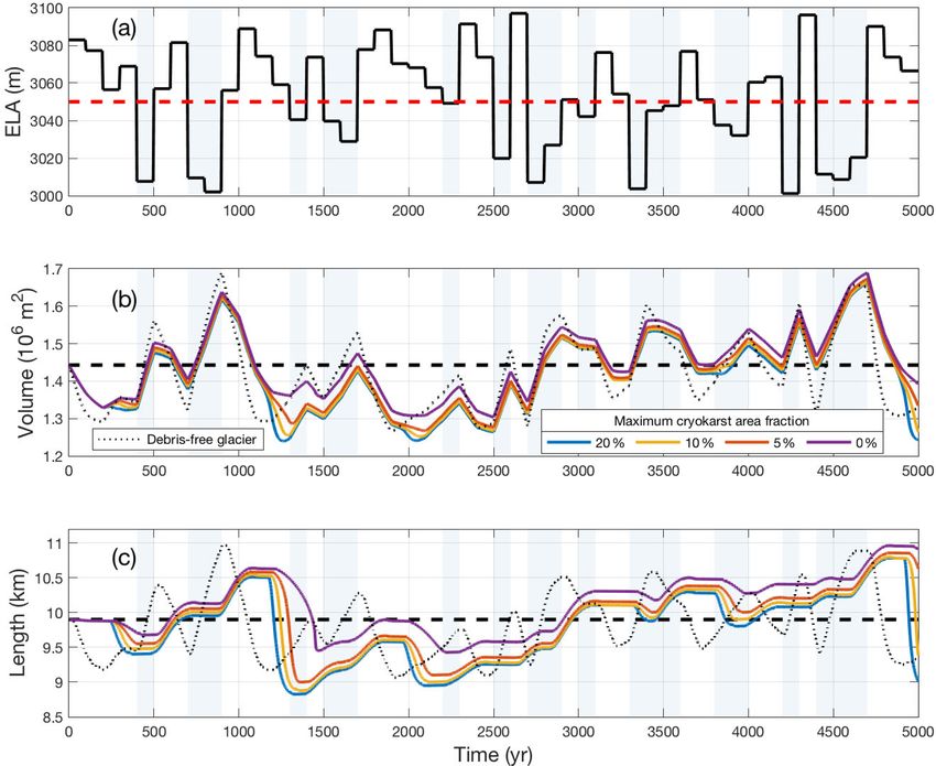
3378                              J. C. Ferguson and A. Vieli: Modelling the transient response of debris-covered glaciers

and supraglacial ponds, which we refer to collectively here as    the transient response and characteristic response times of
cryokarst features, has been suggested as a potential expla-      a debris-covered glacier. A better understanding of how a
nation for this anomalous thinning, and therefore the occur-      debris-covered glacier responds to changes in climate, and
rence of such features and their enhancing effect on surface      what role the debris concentration and the prevalence of
melt have been intensively studied (Sakai et al., 2000, 2002;     cryokarst features play in determining the magnitude of this
Steiner et al., 2015; Buri et al., 2016; Miles et al., 2016).     response, is critical to predicting how today’s debris-covered
However, the influence of dynamic effects on the thinning         glaciers will evolve as the Earth’s climate changes. There-
rates and glacier evolution has so far largely been neglected,    fore, this study aims to fill the gap by investigating the dif-
and such dynamic effects remain poorly understood. Further,       ference in transient response of debris-covered glaciers from
from the reduction in ablation on debris-covered glaciers         their debris-free counterparts. In particular, we (1) examine
a more delayed and dampened response is expected (Benn            how debris cover changes the transient response of an ideal-
et al., 2012). Ideally one would use observational data across    ized glacier to step changes in climate, quantifying both the
a greater temporal and geographical spectrum so that pro-         volume and length response; (2) examine the response to a
cess feedbacks can be observed and examined over relevant         fluctuating climate signal on the long-term evolution of an
timescales. However, the lack of long-term remote sensing         idealized debris-covered glacier as a function of debris con-
data means that we have severe constraints on the availabil-      centration; and (3) examine the impact on mass loss and sur-
ity of such long observational time series, and the recent re-    face evolution when cryokarst features are included, quanti-
construction of Zmuttgletscher (also known as Zmutt Glacier       fying this impact as a function of cryokarst area.
Mölg et al., 2019) provides the only currently available ob-
servable record of a debris-covered glacier that goes beyond
a century.                                                        2     Methods
   Given the paucity of long-term data it is therefore es-
sential to use advanced numerical models in order to in-          2.1     Governing equations
vestigate the role of glacier dynamics on glacier evolution
and mass loss, allowing for the study of interacting pro-         In order to examine the essential features of the interaction
cesses over longer timeframes. Recent progress with numer-        between glacier dynamics and debris cover, we couple an ice
ical simulations of debris-covered glaciers includes Konrad       flow model to a debris transport model that includes both the
and Humphrey (2000), where an early steady-state model of         debris melt-out and its insulating effect on ice ablation. In
debris-covered glaciers was developed; Vacco et al. (2010)        this model, the debris evolution affects the geometry and ice
and Menounos et al. (2013), both of which studied the ef-         flow through changes in the surface mass balance. Our model
fect of a rock avalanche on glacier evolution using a cou-        is similar to that used in Anderson and Anderson (2016) with
pled debris transport and ice dynamics model; Banerjee and        the main differences being some simplifications in the de-
Shankar (2013), which suggested that the transient response       scription of the ice flow, no explicit englacial debris tracking
of a debris-covered glacier to changes in climate has two dis-    within the ice, and the novel option of melt enhancement due
tinct timescales; Rowan et al. (2015), which was the first        to cryokarst features. This cryokarst component is coupled to
modern model of coupled debris-ice dynamics to study the          the flow dynamics and switches on when the tongue becomes
long-term evolution of a debris-covered glacier; and Wirbel       stagnant.
et al. (2018), which tested both 2-D and 3-D advective de-
bris transport using a full-Stokes solver for the ice dynamics.   2.1.1    Ice dynamics
Perhaps the most significant modelling study to date is An-
derson and Anderson (2016), where certain technical issues        For ice flow, we use a flowline version of the shallow ice
are addressed in detail for the first time, such as how to han-   approximation (SIA), a simple model that allows for a real-
dle both the boundary condition at the glacier terminus and       istic qualitative study of a glacier’s response to changing cli-
the possibility of a variable debris source in the accumula-      matic condition. The SIA has been used for studying glacier
tion area. The body of work that uses essentially the same        evolution and response times for debris-free glaciers (e.g.
model has examined diverse topics relating to the feedbacks       Leysinger Vieli and Gudmundsson, 2004), where it achieved
that exist between debris flux, debris thickness patterns, and    comparable results to a full-Stokes solver with significantly
steady-state glacier extent; has also studied the transient re-   less computational time. For a glacier with evolving ice
lationship between debris-covered glaciers and rock glaciers;     thickness H (x, t) flowing along the down-glacier direction
and has been used to explore the processes that govern the        x with depth-averaged velocity u(x, t) in response to a sur-
age of ice-cored moraines (Anderson and Anderson, 2016;           face mass balance forcing a(x, t), the equations for the ice
Crump et al., 2017; Anderson and Anderson, 2018; Ander-           thickness evolution and SIA ice flow are given by
son et al., 2018).
   However, to date no study has used a coupled ice flow-         ∂H ∂(uH )
debris transport model to systematically and in detail study          +     = a,                                              (1)
                                                                   ∂t   ∂x

The Cryosphere, 15, 3377–3399, 2021                                                  https://doi.org/10.5194/tc-15-3377-2021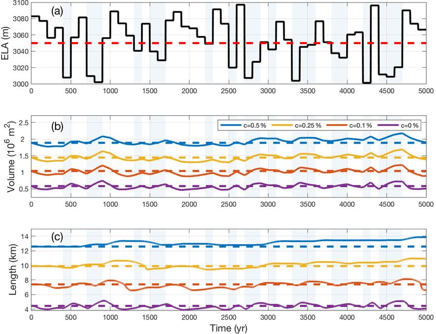
J. C. Ferguson and A. Vieli: Modelling the transient response of debris-covered glaciers                                     3379

                                                                  limits the accumulation to physically realistic values at very
                         n−1                                      high elevations. A surface layer of debris enhances ice abla-
     2A(ρg)n n+1 ∂h            ∂h                                 tion when its thickness D is below a threshold D0 . We ne-
u=          H                     ,                        (2)
      n+2        ∂x            ∂x                                 glect the effect of enhanced ablation when D < D0 and rep-
where ρ is the density of ice, g is gravitational acceleration,   resent the inverse relationship of surface mass balance with
A and n are the rate factor and exponent from Glen’s flow         debris thickness (Anderson and Anderson, 2016) as
law, respectively, and h(x, t) = H + b is the glacier surface               D0
                                                                  a = ã          .                                            (6)
elevation for a given bed elevation b(x). Note that param-                 D0 + D
eter choices in this model will have some effect on the ice
                                                                  The parameter D0 is chosen based on an Østrem curve that is
flow (e.g. a larger value of A will result in smaller glaciers
                                                                  representative for data from Zmuttgletscher, a medium-sized
that respond more quickly to climate forcing) but for reason-
                                                                  Alpine glacier (e.g. Nicholson and Benn, 2006; Mölg et al.,
able values do not significantly change any of the results in
                                                                  2019).
this study. The boundary conditions for the ice thickness H
are handled by specifying a Dirichlet or Neumann boundary         2.1.4     Debris boundary condition at glacier front
condition at x = 0 and requiring that H goes to zero at the
glacier terminus, where the ice front position is a free bound-   The choice of boundary condition at the terminus is of criti-
ary.                                                              cal importance, since the rate at which the supraglacial debris
                                                                  covering the ablation zone leaves the glacier significantly af-
2.1.2   Debris dynamics                                           fects the glacier extent (Anderson and Anderson, 2016), and
                                                                  if this is handled incorrectly, it can lead to runaway glacier
We assume that debris is homogeneously distributed within
                                                                  growth (Konrad and Humphrey, 2000). To ensure that the
the ice with a spatially constant concentration c. The debris
                                                                  boundary condition makes sense, it should be consistent with
melts out when the ice melts at the surface and remains on the
                                                                  observations and should also be grid size independent, since
surface, where it is passively advected with the surface ice
                                                                  the laws of physics should not depend on the choice of dis-
flow velocity us = n+2
                    n+1 u, until it reaches the terminus. The     cretization.
evolution of surface debris thickness D(x, t) is represented
                                                                     With these requirements in mind, we set the boundary con-
by
                                                                  dition such that the debris leaves the system via a terminal
∂D ∂(us D)                                                        ice cliff, as typically observed at termini of debris-covered
   +       = φ,                                            (3)    glaciers (Ogilvie, 1904; see Fig. A1 in Appendix A). This
∂t   ∂x
                                                                  can be achieved most easily through an adjustment of the sur-
where φ is the debris source term at the surface given by         face mass balance, which we adjust at the point where the ice
           (                                                      reaches a critical thickness H ∗ (Fig. A2). All debris melted
             0,      if a ≥ 0
φ(a, H ) =                      .                         (4)     out or transported past this point is assumed to slide off of the
             −ca, if a < 0                                        glacier relatively quickly and is therefore removed from the
                                                                  surface there. This implies that the glacier will always have
Note that for simplicity, we do not account for debris vol-
                                                                  a small debris-free cliff area at the terminus with clean ice
ume changes during melt due to density differences and de-
                                                                  melt. Therefore near the terminus, the surface mass balance
bris porosity; hence our formulation is different by a con-
                                                                  a is given by
stant factor compared to Naito et al. (2000) and Anderson              (
and Anderson (2016). Further, the assumption of uniform de-              ã D0D+D
                                                                               0
                                                                                  , for x < x ∗
bris concentration within the ice means that debris will be       a=                              ,                             (7)
                                                                         ã,         for x ≥ x ∗
present over the entire ablation area, and hence our model
is representative of extensively debris-covered glaciers with     where, as above, ã is the debris-free surface mass balance,
debris deposition in the accumulation area close to the equi-     and x ∗ is the location at which the ice thickness H = H ∗
librium line altitude (ELA) or even extending beyond, into        (with larger x values corresponding to positions further
the ablation area (e.g. Himalaya).                                down-glacier). In addition, we accounted for fact that the
                                                                  near-terminus ice velocity in SIA goes to zero at a faster rate
2.1.3   Surface mass balance                                      than is physically realistic by adjusting the velocity here. The
                                                                  mean velocity from the region up-glacier averaged over 10
We assume that debris-free ice has an elevation-dependent
                                                                  ice thicknesses (here about 300 m) is used when computing
surface mass balance ã given by
                                                                  the debris transport. For more details of the implementation
ã(z) = min {γ (H + b − ELA), amax } ,                     (5)    of the terminus parametrization, see Appendix A.
                                                                     We note that our boundary condition is similar to the one
where γ is the mass balance gradient, ELA is the equilibrium      implemented in Anderson and Anderson (2016), but our ap-
line altitude, and amax is a maximum mass balance, which          proach differs in that we remove debris beyond a critical

https://doi.org/10.5194/tc-15-3377-2021                                                 The Cryosphere, 15, 3377–3399, 2021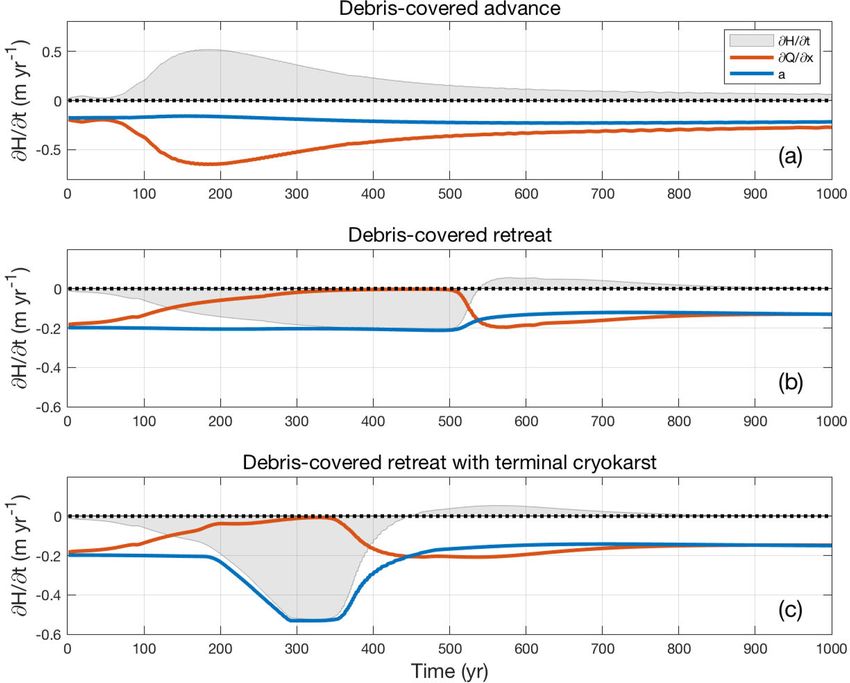
3380 J. C. Ferguson and A. Vieli: Modelling the transient response of debris-covered glaciers
thickness (position of ice cliff), whereas in Anderson and An-
derson (2016) it is removed from a terminal wedge. Although
our ice cliff position is by construction not really grid size
dependent, the modelled terminus position shows some de-
pendency on grid size. However, sensitivity tests demonstrate
that there is fast convergence with decreasing grid size and
the dependency for the 25 m grid size resolution used here
essentially vanishes (see Appendix A, Table A1 and Fig. S6
in the Supplement).
2.1.5 Terminus cryokarst features
For some experiments, we attempt to include the effects of
melt enhancement from cryokarst features. Observations in-
dicate that ice cliffs and supraglacial ponds commonly occur Figure 1. Cryokarst area fraction λ for a range of driving stress
near the termini of stagnating debris-covered glaciers (Pel- values τd for the case of τd− = 60 kPa, τd+ = 110 kPa, and λm = 0.1.
licciotti et al., 2015; Brun et al., 2016; Kraaijenbrink et al.,
2016; Watson et al., 2017) and are associated with regions
that have low driving stresses (Benn et al., 2012). The driv- upper threshold τd+ once the glacier begins to stagnate dur-
ing stress τd , representing the weight of the ice column, is ing retreat. From numerical simulations of retreat, we deter-
given by mined that realistic values for the thresholds are τd+ between
100 and 125 kPa and τd− between 50 and 75 kPa. For more
∂h details, see Appendix B.
τd = ρgH . (8)
∂x
2.1.6 Model setup numerical implementation
Using such a dynamic coupling as a first approximation, we
couple the initiation of cryokarst features to driving stresses The coupled dynamic system described above is solved us-
below a threshold value. Specifically, we define two driving ing standard finite differences and discretizations for the ice
stress thresholds, a maximum τd+ and a minimum τd− , and we flow, similar to that first described by Mahaffy (1976), cou-
introduce a local cryokarst area fraction λ which represents pled with centred differences for the debris transport. Care
the debris-free area associated with ice cliffs and supraglacial is taken to ensure that each time step fulfills the Courant–
ponds. For a driving stress above τd+ , the local cryokarst area Friedrichs–Levy (CFL) condition, which is necessary for the
fraction λ is set to zero, which corresponds to no ice cliffs numerical stability of the method (Courant et al., 1928). Es-
and no supraglacial lakes. For a driving stress below τd− , the sentially, the CFL condition limits the length of each time
local cryokarst area fraction equals a maximum value λm . For step so that information from any computational cell can
driving stress values in between the thresholds, we assume propagate only as far as its nearest neighbours. Importantly,
the local cryokarst contribution is linear in λ, given by the boundary condition at the glacier terminus requires in-
terpolation to determine the exact location of the critical ice
0,
if τd+ ≤ τd thickness H ∗ and to weight the surface mass balance forcing
λ = λm (τd+ − τd )/(τd+ − τd− ), if τd− < τd < τd+ . (9) accordingly in the corresponding grid cell.
if τd ≤ τd−
λm , In the results that follow, all computations are performed
using a bed consisting of a headwall with a slope of 45◦ fol-
This dependence of cryokarst area fraction on driving stress lowed by a linear bed with a slope of roughly 6◦ . All model
is illustrated in Fig. 1 for τd− = 60 kPa, τd+ = 110 kPa, and constants are shown below in Table 2.
λm = 0.1.
For the fraction of area where cryokarst is present, we as-
sume that there is no longer an insulating effect on the surface 3 Modelling results
mass balance. Adjusting the local surface mass balance a to
account for this gives Our goal is to better understand how the transient response of
a debris-covered glacier is different than that of a debris-free
D0 glacier and what effect cryokarst features have on this tran-
a = λã + (1 − λ)ã . (10) sient response. To do this, we perform a series of numerical
D0 + D
experiments consisting of applying step changes or random
The threshold values τd+ and τd− are based on the values of climate histories in the climate forcing for glaciers with vari-
the driving stress during advance and retreat in the cryokarst- able debris concentration and hence various levels of surface
free case and are chosen such that τd only drops below the debris and analyze the resulting volume and length response.
The Cryosphere, 15, 3377–3399, 2021 https://doi.org/10.5194/tc-15-3377-2021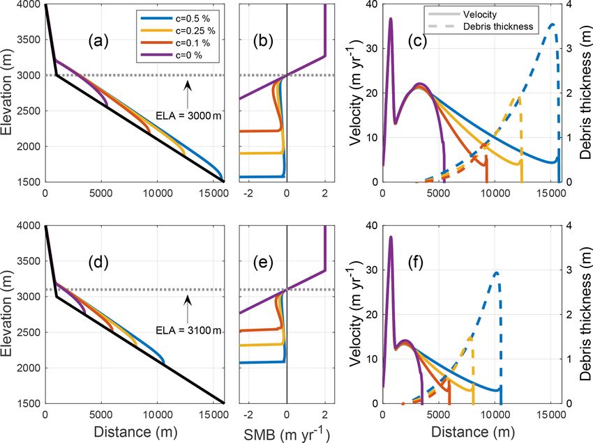
J. C. Ferguson and A. Vieli: Modelling the transient response of debris-covered glaciers                                        3381

Table 1. Summary of modelling experiments performed.

                        No.    Description                                                   Section   Figures
                        0      Baseline: steady states at ELA = 3000, 3100 m                   3.1     2
                        1      Transient response due to step change between steady states     3.2     3, 4, 5
                        2      Random climate forcing                                          3.3     6
                        3      Transient response with cryokarst                               3.4     7, 8
                        4      Random climate forcing with cryokarst                           3.5     9

   First we examine the steady-state case for two climates            at the ELA) and hence independent of debris concentration.
and four different debris concentrations in Sect. 3.1. Then in        The surface mass balance for the debris-covered glaciers no
Sect. 3.2, we examine the transient behaviour of glaciers that        longer decreases linearly with elevation but is instead con-
move from one steady state to another after a step change             trolled primarily by the debris thickness and strongly reduced
in climate for the case of debris concentration c = 0.25 %.           over most of the ablation area, as shown in Fig. 2b and e.
Next, we simulate a random climate forcing for a duration             Surface velocities generally decrease with increasing debris
of 5000 years for glaciers with different debris concentra-           thickness along the glacier, as seen in Fig. 2c and f.
tions and examine the resulting transient volume and length              An interesting observation here is that for a fixed climate,
response, found in Sect. 3.3. We next examine the effect of           the debris thickness profile in steady state appears to be ap-
introducing cryokarst features near the terminus on the tran-         proximately independent of concentration, while the glacier
sient response to a step change in climate in Sect. 3.4. Finally,     extents differ strongly. This is discussed further in Sect. 4.5.
we have a second look at the transient response to random
climate forcing when cryokarst is present in Sect. 3.5. An            3.2   Transient response between steady states
overview of these experiments is found in Table 1, with ref-
erence to the relevant figures in the text. Table 2 summarizes        Next we analyze the response to a step change in the cli-
the parameter values used in the numerical model.                     mate forcing. Figure 3 shows the transient volume and length
                                                                      changes due to ELA step changes of ±100 m. In Fig. 3b,
3.1   Steady-state glacier extent                                     glacier volume time series show the response time depen-
                                                                      dence on debris concentration, with the expected result that
As a baseline for understanding the glacier’s response to             higher debris concentration leads to a longer volume re-
a changing climate, we first examine steady-state features            sponse time. Here, filled-in squares denote the e-folding vol-
for the two climate extremes of our study, ELA = 3000                 ume response time (Jóhannesson et al., 1989; Oerlemans,
and 3100 m, which are representative of the climate for a             2001), which is the time it takes to reach 1 − 1/e ' 63 % of
medium-sized Alpine glacier during the last century. Al-              the total volume change. The values of the numerical volume
though in reality glaciers never attain a true steady state           response time are shown in Table 3 in the columns marked
due to a constantly changing climate, equilibrium conditions          Tnum . In general, the volume response times are strongly in-
are useful for theoretical studies because they provide well-         creased for debris-covered glaciers compared to the debris-
understood rest states around which glacier fluctuations can          free case. A more detailed discussion of volume response
be more easily studied. As for debris-free glaciers, a steady         time follows in Sect. 4.3.
state is defined as the point at which, for a fixed climate, the         In Fig. 3c, the length times series allow for a compari-
glacier geometry no longer changes with time. Additionally,           son with the length response time. For the case of glacier
in our modelling there is a further requirement that the debris       advance, shown on the right side of the plot starting at
flux entering the glacier also must leave the glacier surface at      T = 1000 years, the form of the length change is similar to
the terminus.                                                         that of the volume change: a slow but steady increase leading
   Figure 2 shows the steady-state glacier surface and bed            asymptotically to a steady state. However, the retreat phase,
profiles, velocity profiles, and debris thickness profiles for        shown for T = 0 to 1000 years, is contrasting this response
the debris-free case as well as for the debris concentrations of      behaviour. Here, we see a clear lag in length response, which
c = 0.1 %, 0.25 %, and 0.5 %. The glacier profiles in Fig. 2a         gets stronger for larger debris concentrations. The lag is so
and d show the expected behaviour of higher debris concen-            pronounced that when the glaciers have reached their respec-
tration leading to longer, larger glaciers. A debris concen-          tive e-folding volumes, denoted as filled-in squares, they are
tration of only 0.1 % almost doubles the glacier length com-          still approximately at their pre-step change extent.
pared to the clean ice case. Note that the glacier geometry              To show the difference in length versus volume response
in the debris-free part above the ELA is almost identical for         more clearly, we closely examine one debris-covered glacier,
all cases (with a small difference when greater debris cover          with c = 0.25 % debris concentration, and contrast its re-
results in a more elongated glacier with a lower surface slope        sponse with the debris-free case. In Fig. 4, the normalized

https://doi.org/10.5194/tc-15-3377-2021                                                      The Cryosphere, 15, 3377–3399, 2021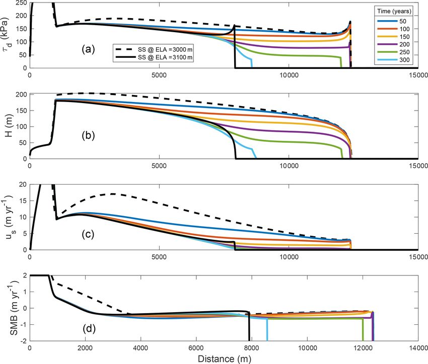
3382                                  J. C. Ferguson and A. Vieli: Modelling the transient response of debris-covered glaciers

Table 2. Values used for the model parameters.

                              Parameter     Name                                                Value     Units
                              ELA           Equilibrium line altitude                     3000–3100       m
                              ρ             Density of ice                                        910     kg m−3
                              g             Gravitational acceleration                           9.80     m s−2
                              c             Debris volume concentration                      0–0.005
                              A             Flow law parameter                             1 × 10⁻²⁴      Pa−3 s−1
                              n             Glen’s constant                                          3
                              D0            Characteristic debris thickness                      0.05     m
                              amax          Maximum surface mass balance                             2    m yr−1
                              γ             Surface mass balance gradient                       0.007     yr−1
                              H∗            Terminal ice thickness threshold                        30    m
                              λm            Maximum cryokarst fraction                          0–0.2
                              dt            Time step                                            0.01     yr
                              dx            Spatial discretization                                 25     m
                              τd+           Upper cryokarst driving stress threshold         100–125      kPa
                              τd−           Lower cryokarst driving stress threshold           50–75      kPa
                              θ             Bed slope                                              0.1    m m−1
                              θc            Headwall slope                                           1    m m−1

Figure 2. Steady-state glacier geometry profiles (a, c), and profiles of surface velocity (solid lines) and debris thickness (dashed lines) (b, d),
corresponding to ELA = 3000 and 3100 m for four different debris concentrations.

volume and length are plotted together for each glacier,                    sponse and the length response, which is more evident dur-
where we have set the cold (ELA = 3000 m) steady-state                      ing retreat. The debris-covered response, in Fig. 4b, shows
volume V = 1 (length L = 1) and warm (ELA = 3100 m)                         a substantial lag time between the volume response and the
steady-state volume V = 0 (warm length L = 0) for ease of                   length response. This lag in the length response is, at roughly
comparison. For the debris-free case, shown in Fig. 4a, the                 250 years, much larger during the retreat but is also observ-
volume and length curves follow each other closely but there                able during the advance, where a 50-year lag is observed
is a small but noticeable time lag between the volume re-                   at the onset of advance. An additional difference between

The Cryosphere, 15, 3377–3399, 2021                                                               https://doi.org/10.5194/tc-15-3377-2021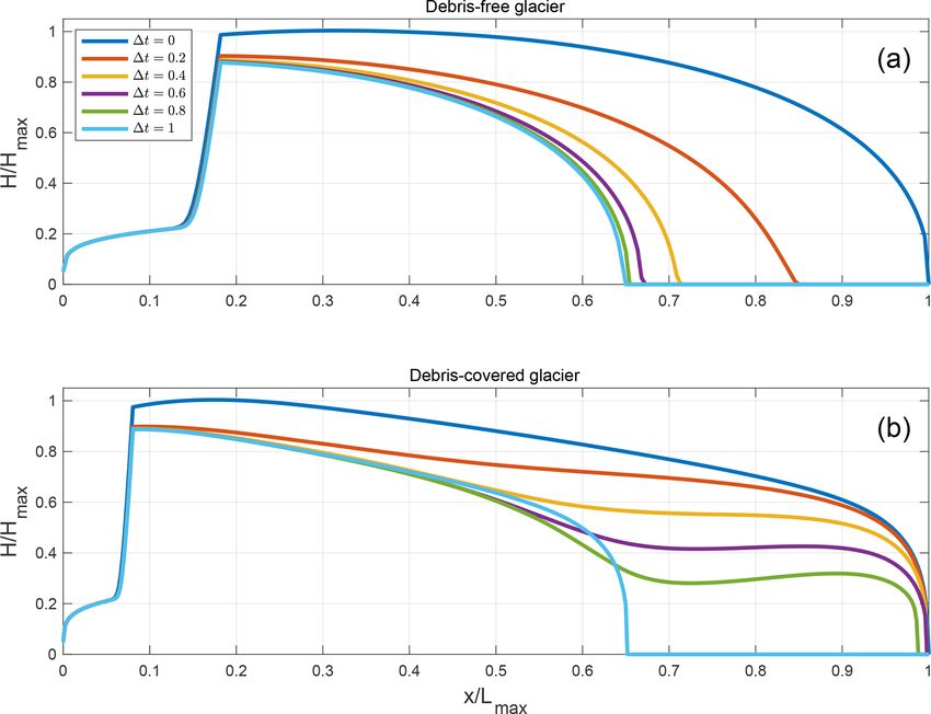
J. C. Ferguson and A. Vieli: Modelling the transient response of debris-covered glaciers                                                3383

Table 3. Comparison of numerical e-folding volume response times (in years) due to step changes between steady states at ELA = 3000 and
ELA = 3100 m for different debris concentrations. The columns marked Tnum represent the numerical volume response time, and the other
columns represent the theoretical estimate of Jóhannesson et al. (1989) developed for clean ice using different methods of calculating the
surface mass balance at the terminus (see Sect. 4.4 for details).

                                c                 τv – retreat                         τv – advance
                                        Tnum    T1     T2        T3   T4     Tnum     T1      T2      T3   T4
                                0         77     52    –          –    –      133    108       –      –     –
                                0.1      154     29   456        54   222     265     48     694      87   340
                                0.25     256     22   646        42   207     396     34     955      66   321
                                0.5      385     17   800        34   179     529     25    1237      50   273

Figure 3. Step change in ELA between steady states (a) leading to transient volume response (b) and transient length response (c) for glaciers
with different debris concentrations (coloured lines). The filled-in squares in both (b, c) represent the e-folding volume response time.

the glaciers is found near the end of the retreat phase. The                tive transient evolution times during retreat for both glaciers.
transient debris-covered glacier volume overshoots the fi-                  In Fig. 5a, we see that immediately as the debris-free glacier
nal steady-state volume, observable starting just before T =                thins, it also retreats in a roughly uniform way with thin-
500 years in Fig. 4b, before recovering to its final volume.                ning approximately matched by reduction in glacier extent.
During this overshoot and recovery in volume, the transient                 This can be thought of as a manifestation of a volume-area
glacier length monotonically decreases and never goes below                 scaling law V = cAγ (e.g. Bahr et al., 1997), which essen-
its final steady-state length. In contrast, the transient debris-           tially says that a debris-free glacier volume is linked to its
free glacier volume has no overshoots: it monotonically de-                 area by a power law. Note that for our flowline model, the
creases during retreat.                                                     equivalent scaling law is a relationship between area and
   In Fig. 5, we again compare the debris-free case with the                length. The debris-covered glacier profile shown in Fig. 5b
c = 0.25 % debris-covered case, but this time we look at the                does not follow the same pattern. As the glacier thins dur-
respective glacier thickness profiles during retreat. To facil-             ing the period of relative time 1t = 0 to 1t = 0.6, there is
itate comparison across spatial and temporal scales, we plot                no discernible change in the glacier extent. Initially, most of
the normalized glacier thickness profiles for equivalent rela-              the thinning occurs in the upper half of the ablation zone

https://doi.org/10.5194/tc-15-3377-2021                                                            The Cryosphere, 15, 3377–3399, 2021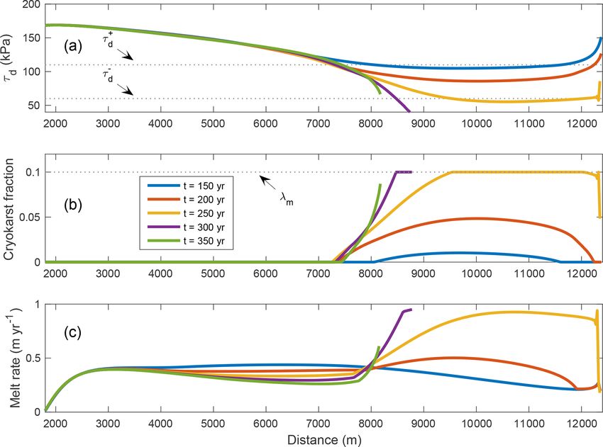
3384 J. C. Ferguson and A. Vieli: Modelling the transient response of debris-covered glaciers
Figure 4. Normalized transient volume and length response for a step change in ELA between two steady states for (a) a debris-free glacier
and (b) a debris-covered glacier with c = 0.25 %.
but ceases there rapidly after 1t = 0.1 to 0.2 relative time. vals of 100 years, which is close to but a bit larger than the
By 1t = 0.6, the entire region from relative length x = 0 to clean ice response time during retreat, and they have a mean
x = 0.6 is at or slightly below its final steady-state ice thick- of ELA= 3050 m. This random climate forcing is shown in
ness even though the original glacier extent has not changed Fig. 6a, and the respective transient volume and length time
yet. Only by 1t = 0.8 do we finally see the glacier termi- series are shown in Fig. 6b and c for a debris-free glacier and
nus start to retreat, with the last roughly 35 % of the glacier three debris-covered glaciers with different debris concentra-
appearing as a thin, not very dynamic, and soon to be dis- tions.
connected terminus (see Fig. S1 for corresponding velocity The behaviour of the debris-free glacier (purple line at the
profiles). Although the velocity is nonzero, this type of ter- bottom of Fig. 6b and c) exhibits a relatively rapid volume
minus is often described as stagnating because dynamic re- and length response, which can be seen by how quickly the
placement of ice is close to zero, and hence the local thinning solid curve, representing the transient, moves back towards
rate is roughly equal to the local surface mass balance. The the dashed line, which represents the steady-state value for
loss of this stagnant terminus results in a large, rapid decrease the mean climate of ELA = 3050 m. For the debris-covered
in ice volume and a corresponding rapid retreat (e.g. the blue glaciers with lower concentration (red and yellow lines in
curves in Fig. 3b and c at around t = 600 years). In the final Fig. 6b), the volume responds only marginally more slowly.
20 % of the total retreat time, the stagnant terminus has com- The difference is more pronounced for the glacier with the
pletely disappeared and the central region that had previously greatest debris concentration (blue line), where the transient
over-thinned has now recovered to its steady-state thickness volume never goes below the mean climate steady-state vol-
and has become the new terminus. We revisit this interesting ume beginning from T = 2800 years. Note that the light blue
terminus behaviour in Sect. 4.1 below. shading corresponds to colder-than-average time periods and
white shading corresponds to warmer-than-average time pe-
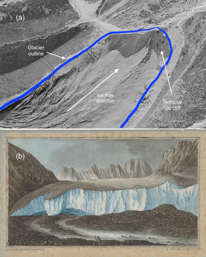
3.3 Response to random climate forcing riods.
The asymmetric response is much more pronounced in
We have investigated debris-covered glacier response to step the transient length time series. While the glacier with the
changes in the climate, and it is natural to query whether lowest debris concentration (red line in Fig. 6c) exhibits a
these results will have any bearing on a more realistic fluc- marginally slower response compared to the debris-free case
tuating climate input. To investigate this issue in a some- (solid purple line), the glaciers more heavily laden with de-
what less idealized setting, we initialize the model to a steady bris, shown in yellow and blue, have transients lengths that
state corresponding to an ELA of 3050 m. Then we force the are almost throughout more extended than the mean climate
model using a varying climate signal consisting of a 5000- steady-state length and tend to advance more than retreat.
year long time series made up of random fluctuations be- This is especially true for the c = 0.5 % case, which after
tween ELA= 3000 m and ELA= 3100 m, which corresponds 5000 years is more than 1 km longer than one would expect
in the Alps to a change in air temperature of about 0.8 ◦ C for the mean value climate. Hence, due to the lag in the length
(Linsbauer et al., 2013). The fluctuations occur at fixed inter-
The Cryosphere, 15, 3377–3399, 2021 https://doi.org/10.5194/tc-15-3377-2021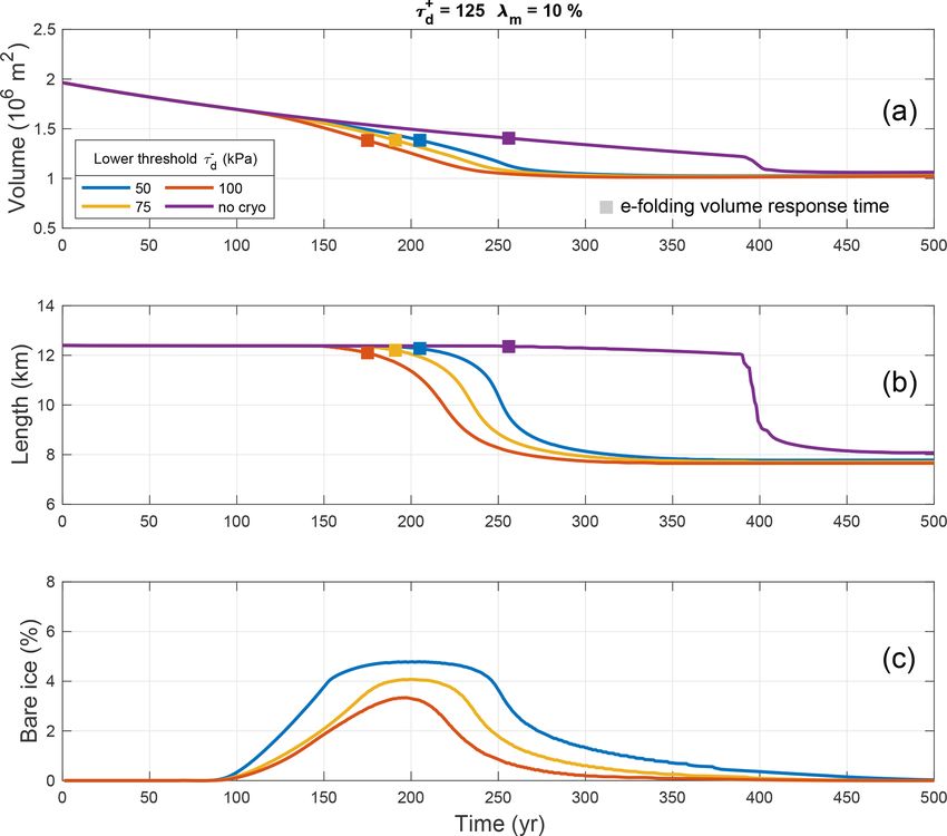
J. C. Ferguson and A. Vieli: Modelling the transient response of debris-covered glaciers                                                      3385

Figure 5. Glacier thickness profiles relative to the maximal initial thickness for (a) a debris-free glacier and (b) a debris-covered glacier with
c = 0.25 % at different times during a transient retreat. The different coloured lines refer to the time relative to the time it takes to retreat to
steady state, where a time of t = 0.1 corresponds in the debris-free case to about 38 years and in the debris-covered case to about 40 years.

Figure 6. Random climate forcing (a) and the corresponding transient volume response (b) and transient length response (c) for glaciers of
different debris concentrations. The dashed lines represent (a) the mean value climate of ELA = 3050 m and the corresponding steady-state
(b) volume and (c) length. The light blue background shading represents temporal periods during which the climate forcing is colder than
the mean climate.

https://doi.org/10.5194/tc-15-3377-2021                                                              The Cryosphere, 15, 3377–3399, 2021
3386 J. C. Ferguson and A. Vieli: Modelling the transient response of debris-covered glaciers
response to a warming climate, debris-covered glaciers pref- Table 4. Comparison of numerical e-folding volume response times
erentially show the effects of the colder climate. Put another (in years) due to step changes between ELA = 3000 m and ELA =
way, debris-covered glaciers remember periods of cold cli- 3100 m for a debris concentration of c = 0.25 % and with the pres-
mate more than warm ones. This also suggests that the time- ence of several different values of maximum terminal cryokarst
averaged length of a debris-covered glacier under random cli- fraction λm .
mate forcing will be longer than the steady-state length for
Debris conc. c Max. cryo. Vol. resp.
the equivalent constant climate forcing.
fraction λm time τv
3.4 Effect of cryokarst on response 0.25 0 256
0.25 0.05 234
Most of the debris-covered glaciers observed in the present 0.25 0.1 219
day have varying amounts of ice cliffs and supraglacial ponds 0.25 0.2 200
present on their tongues which are known to enhance surface
ablation (Benn et al., 2012). However, the long-term effect of
such cryokarst features on thinning and glacier dynamics is steps, spaced 50 years apart, corresponding to the case of
poorly understood. With this in mind, we repeat the above ex- λm = 10 %. As the driving stress drops below the upper
periments for four debris-covered glaciers, all with a medium threshold τd+ , shown in Fig 8a, the cryokarst area fraction
debris concentration c = 0.25 % by including the dynamic is observed to increase, shown in Fig 8b. This leads to an in-
cryokarst model introduced in Sect. 2.1.5 and perform runs crease in melt rate, depicted in Fig 8c. The maximum melt
for the different maximum local cryokarst area fraction of rates occur at t = 250 and 300 years, shown in yellow and
λm = 0 %, 5 %, 10 %, and 20 % (consistent with observa- purple, when the driving stress is at or below the lower
tions from Mölg et al., 2019; Steiner et al., 2019; Ander- threshold τd− and the corresponding cryokarst area fraction
son et al., 2021). Driving stress thresholds of τd+ = 110 kPa λ at the terminus achieves the maximum value λm . This in-
and τd− = 60 kPa are used here. Since we dynamically couple creased melt rate contributes to a rapid retreat, corresponding
the onset and intensity of melt enhancement from cryokarst to the green line for t = 350.
to the driving stress using Eqs. (9) and (10), the effect of
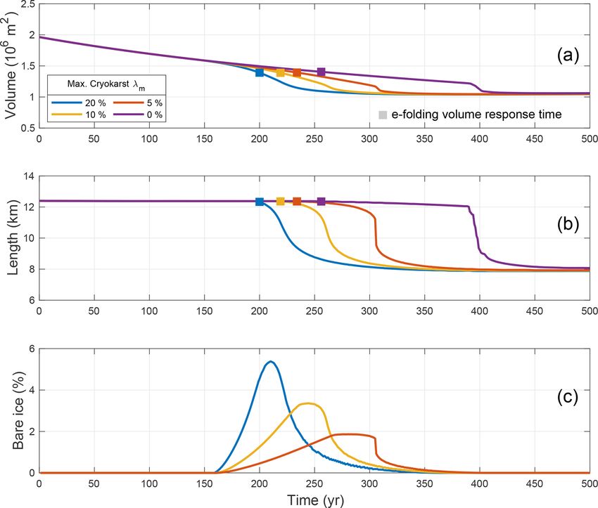
cryokarst is only felt during periods of mass loss, and we fo- 3.5 Response to random climate forcing with presence
cus exclusively on this in Fig. 7. The purple lines in Fig. 7a of cryokarst
and b correspond to the case with no cryokarst features, and
therefore they show the same retreat as the yellow lines in Figure 9 shows the same random climate forcing experiment
Fig. 3b and c. with c = 0.25 % as in Fig. 6 but cryokarst with driving stress
The addition of cryokarst has a noticeable effect on both thresholds of τd+ = 110 kPa and τd− = 60 kPa, as well as four
the volume and length response of a debris-covered glacier. different maximum local cryokarst area fractions λm = 0 %,
In Fig. 7a, there is a clear reduction visible in the e-folding 5 %, 10 %, and 20 %. As before, the λm = 0 glacier, corre-
volume response time of a couple of decades (see Table 4 for sponding to the purple curves in Fig. 9, is identical to the
the exact values), which is more pronounced with the pres- results already plotted in Fig. 6 in yellow. Since there is no
ence of enhanced cryokarst. The effect on glacier length re- dynamical effect during periods of advance, we do not see
sponse is even more striking, with a difference of more than much difference in either the volume or length change rate in
a century between the timings of the onset of retreat. The ac- colder climate regimes; see in particular between 3000- and
tual amount of equivalent bare ice for each glacier is shown 5000-year model time. However, during retreat the difference
as a percentage of the entire ablation zone area in Fig. 7c. is visible especially during the warm-climate-dominated pe-
Even for the smallest amount of cryokarst modelled, which riod of T = 1300 to 3000 years. In Fig. 9b and even more
accounts for only 2 % of equivalent bare ice in the ablation clearly in Fig. 9c, the transient volume and length of the
area, there is a shortening of roughly 70 years in the timing cryokarst-covered glaciers exhibit a shorter memory and are
of the main phase of retreat. Despite this evident effect the therefore able to retreat much more quickly than the corre-
presence of cryokarst has on length response, there is still a sponding cryokarst-free glacier. Despite this faster response,
significant lag observed compared to the clean ice case, as all of the modelled debris-covered glaciers still respond with
in all modelled cases the glaciers are still at their maximum much more delay than a debris-free glacier with the same
pre-step change extents even by the respective e-folding vol- climate forcing, as shown in the black dotted line in Fig. 9b
ume response times. Note that the choice of driving stress and c, which has been rescaled in the magnitude for both
thresholds affects the strength of the cryokarst effect on the length and volume for ease of comparison. As noted above,
response (see Figs. S2 and S3). the timing in onset of retreat is rather sensitive to the choice
To aid in the visualization of the effect of cryokarst on the of the upper and lower driving stress thresholds. To compare
transient glacier dynamics, we plot driving stress, cryokarst with results using different threshold values, please refer to
area fraction, and melt rate in Fig. 8 at five different time Figs. S4 and S5.
The Cryosphere, 15, 3377–3399, 2021 https://doi.org/10.5194/tc-15-3377-2021J. C. Ferguson and A. Vieli: Modelling the transient response of debris-covered glaciers 3387
Figure 7. Transient volume response (a) and length response (b) for debris-covered glaciers with terminal cryokarst features retreating from
steady state after a 100 m step change in ELA. Each colour represents a different value of the maximum cryokarst percentage λm . In all
cases, the debris concentration is c = 0.25 %, and the driving stress thresholds are τd+ = 110 kPa and τd− = 60 kPa. The filled-in squares in
panels (a) and (b) represent the e-folding volume response time. The percentage of total debris-covered length that has a bare ice equivalent
surface mass balance due to the presence of cryokarst is shown in panel (c).
4 Discussion primarily interested in the retreat rate. Figure 10 shows the
components of the mass conservation Eq. (1) for the moving
We explored the transient response of a debris-covered region consisting of the last 200 m of debris-covered area for
glacier to changes in climate forcing using a flowline model the cases of advance, retreat, and retreat with maximum local
that couples ice flow with debris melt out and advection and cryokarst area fraction λm = 5 % and driving stress thresh-
also includes an ad hoc representation of the effects of dy- olds τd+ = 110 kPa and τd− = 60 kPa. The initial condition for
namically coupled cryokarst features at the glacier terminus. all three panels is steady state for an ELA = 3050 m, with the
Several interesting results related to dynamics were obtained, advance and retreat due to ELA step changes of ±50 m at
which we discuss separately in light of observational data, T = 0.
previous studies, and model limitations. In each plot, the grey region represents the thickening or
thinning rate, with the area under the curve representing the
4.1 Terminus behaviour during transient response total thickness change of the last 200 m during the entire
1000 years of the advance or retreat. In all three cases, dur-
The results of our numerical experiments indicate that debris- ing the first 200 years the surface mass balance a, plotted in
covered glaciers have an asymmetric response to climate blue, does not change appreciably from the pre-step change
forcing, with a visible lag in response during a retreat, and value of a = −0.2 m yr−1 . This is because the debris at the
that the magnitude of the lag is reduced in the presence of ter- terminus is thick enough to make the glacier here relatively
minal cryokarst. To better understand this behaviour, we fur- insensitive to small changes in climate forcing. For the ad-
ther examine the debris-covered terminus region during ad- vancing glacier, depicted in Fig. 10a, the change in surface
vance and retreat and consider the relative magnitudes of sur- mass balance is minimal and the thickening rate is driven by
face mass balance a and flux divergence ∂Q/∂x on the rate of an increase in the magnitude of the flux divergence (red line),
thickness change ∂H /∂t. Anderson et al. (2021) used a simi- which peaks at around T = 150 years, the time taken for the
lar approach to study thinning at the terminus, but here we are
https://doi.org/10.5194/tc-15-3377-2021 The Cryosphere, 15, 3377–3399, 20213388 J. C. Ferguson and A. Vieli: Modelling the transient response of debris-covered glaciers
Figure 8. Profiles of driving stress (a), cryokarst fraction (b), and melt rate (c) at five different time steps for the case of maximum cryokarst
area fraction λm = 10 %. The dashed lines in panel (a) denote the driving stress thresholds used in the cryokarst parameterization.
increased ice flux to propagate down the glacier to the termi- 4.2 Debris-covered glacier memory
nus.
For the retreating glacier, shown in Fig. 10b, the thin- We showed that the memory of a debris-covered glacier is se-
ning rate is clearly driven by a decrease in flux divergence, lective, exhibiting an effective hysteresis, with periods of rel-
which eventually drops to zero at roughly T = 300 years, at atively cold climate having a sustained effect on the volume
which point the glacier terminus stagnates. It remains so un- and in particular on the length. Strictly speaking this is not a
til roughly T = 500 years, when the total amount of thin- true hysteresis since if the glacier is allowed a lengthy relax-
ning, almost equal to the local surface mass balance, is large ation period of several centuries, the resulting equilibrium is
enough that the stagnant terminus finally disappears. After independent of history. Some previous numerical simulations
this, there is a small amount of thickening at the terminus as of the transient response of debris-covered glaciers focused
the glacier readjusts to the overshoot caused by the collapse only on the effects of sudden debris input in the form of an
of the stagnant terminus. avalanche (Vacco et al., 2010; Menounos et al., 2013). Such
When a small amount of cryokarst features is added to a one-time debris input leads to an advance in glacier extent
the terminus during retreat, representing at most roughly 2 % and foreshadows the results of our study, where a constant
of the total debris-covered area (Fig. 10c), the glacier be- debris source and changing climate forcing gives rise to a
haves identically to the cryokarst-free case up until roughly more complex response.
T = 190 years. From then on the terminus dynamics become The glacier termini seem to struggle to retreat in warmer
stagnant enough that the cryokarst features begin to develop periods even if they are sustained over a century, and hence
and within several decades cause an increase in the melt rate debris-covered glaciers have the tendency to either advance
by a factor of more than 2. This significantly speeds up the or stagnate in a century-scale fluctuating climate (Fig. 6).
thinning on the tongue and hence the retreat rate, with the This also means that for debris-covered glaciers, no unique
bulk of the retreat completed about 100 years earlier than in glacier length exists for a given climate but rather that the
the cryokarst-free case. length of debris-covered glaciers is determined by the his-
tory of repeated cold phases. Furthermore, debris-covered
glaciers under random climate forcing are expected to have
a longer average length than the steady-state length corre-
sponding to the equivalent constant climate forcing. These
The Cryosphere, 15, 3377–3399, 2021 https://doi.org/10.5194/tc-15-3377-2021J. C. Ferguson and A. Vieli: Modelling the transient response of debris-covered glaciers 3389 Figure 9. Random climate forcing (a) and the corresponding transient volume response (b) and transient length response (c) for glaciers of different maximum cryokarst fraction λm . The dashed lines represent (a) the mean value climate of ELA = 3050 m and the corresponding steady-state (b) volume and (c) length. The light blue background shading represents temporal periods during which the climate forcing is colder than the mean climate. In all cases, the debris concentration is c = 0.25 %, and the cryokarst driving stress thresholds are τd+ = 110 kPa and τd− = 60 kPa. are novel modelling results which have important implica- change and hence average thinning behaviour are surpris- tions not only for the observed present-day extended extents ingly similar for all debris concentrations and the clean ice of debris-covered glaciers but also on historical reconstruc- case (Fig. 6), which agrees with the general observations of tions. For example, inferences of past climate from historical relatively high mass loss despite the occurrence of substan- glacier extents that do not take into account the asymmet- tial debris cover (Pellicciotti et al., 2015; Brun et al., 2018). ric memory of debris-covered glaciers risk misrepresenting Such rapid mass loss is governed by two processes. Initially, the climate as being colder than it actually was (Clark et al., the warming has a strong impact on the upper accumulation 1994). area where debris is still thin. Then the lower tongue with Observational data (Quincey et al., 2009; Scherler et al., thick debris cover stagnates and dynamic ice replacement di- 2011; Ragettli et al., 2016) show that many debris-covered minishes (∂Q/∂x goes to zero, Fig. 10b), and hence the ice glaciers have strongly extended and stagnating tongues, simply melts away. As this stagnant area is extensive the re- which is consistent with our modelling and our interpretation lated total volume loss is therefore substantial. that debris-covered glaciers remember rather the colder cli- The results presented used a random climate forcing with mates of the past, and are therefore quite far out of balance a particular ELA range and time interval between random with the present climate. However, since the observational step changes. Different climate forcing signals are possible, record is not long enough to provide data on meaningful as are many different shapes and sizes of glaciers with vary- timescales and is heavily biased towards retreating glaciers, ing debris thickness profiles. However, the general qualita- it is currently only possible to study this phenomenon fully tive results are expected to be the same, though for exam- using numerical experiments. ple a longer time interval between random steps (approach- Note that this asymmetric response to climate forcing is ing the debris-covered response time) will reduce the debris- much more pronounced for the adjustment in glacier length covered memory effect. This is indicated in the random cli- than in volume. In the random climate experiments, volume mate experiments by the ability of the terminus to retreat https://doi.org/10.5194/tc-15-3377-2021 The Cryosphere, 15, 3377–3399, 2021
3390                                 J. C. Ferguson and A. Vieli: Modelling the transient response of debris-covered glaciers

Figure 10. Thinning rate, flux divergence, and surface mass balance averaged over the final 200 m of the glacier terminus before the terminus
during advance (a), retreat (b), and retreat with cryokarst (c), for c = 0.25 %, λm = 0.05, τd+ = 110 kPa, and τd− = 60 kPa. In all cases, the
initial condition is a steady state at ELA = 3050 m followed by a 50 m step change in ELA at time t = 0.

in response to several successive warm periods (several cen-             consequence of our rather ad hoc approach and threshold for
turies), as shown in Fig. 6. An obvious extension of this work           the onset of cryokarst.
is to undertake a detailed sensitivity analysis, using a variety            Numerous previous studies (Sakai et al., 2000, 2002; Benn
of climate signals, glacier geometries, and debris thickness             et al., 2012; Buri et al., 2016; Kraaijenbrink et al., 2016;
profiles, in order to better understand the conditions under             Miles et al., 2016; Ragettli et al., 2016; Watson et al.,
which this selective memory effect becomes significant.                  2017; Rounce et al., 2018) have investigated the role of ice
                                                                         cliffs and supraglacial ponds on the enhancement of melt on
4.3    Cryokarst effect in modulating response                           debris-covered glaciers and indicate some link between stag-
                                                                         nation in ice dynamics and the development of such cryokarst
                                                                         features. Our model is, however, the first attempt to couple
Our results suggest that cryokarst features which dynam-                 the effects of these features to glacier dynamics in a numeri-
ically develop during a retreat on the stagnating terminus               cal model in order to explore the impact on glacier thinning.
substantially speed up the length response and also notice-              Although the ad hoc approach used here is admittedly sim-
ably reduce the volume response time. This is important for              plistic, it does allow for the general effect of cryokarst to
any long-term modelling studies involving debris-covered                 be incorporated dynamically without requiring knowledge of
glaciers, as neglecting the effects of cryokarst results in an           the details of the physical processes, which are not yet com-
overestimation of transient response times during a warming              pletely worked out and would greatly complicate the numer-
phase. Furthermore, the resulting earlier and more enhanced              ics since they are occurring at the sub-grid scale. The param-
mass loss rates agree better with the current observations of            eters chosen resulted in behaviour consistent with fractional
rapid thinning (Pellicciotti et al., 2015; Brun et al., 2018;            area observations (Mölg et al., 2019; Steiner et al., 2019; An-
Mölg et al., 2019), but the terminus response is still strongly          derson et al., 2021, give a local area fraction up to 12 %),
delayed and requires warm periods of substantial durations               and the approximate timing of the cryokarst evolution also
(several centuries) to cause substantial retreat (Fig. 9). This          matches the observation that stagnating glaciers tend to have
suggests that today’s thinning may still be related to the               more cryokarst (Benn et al., 2012).
warming after the Little Ice Age, or, alternatively, it may be a

The Cryosphere, 15, 3377–3399, 2021                                                            https://doi.org/10.5194/tc-15-3377-2021
J. C. Ferguson and A. Vieli: Modelling the transient response of debris-covered glaciers 3391
The main limitation to this component of the model is vance are found in Table 3. As is evident by comparison with
that the choice of driving stress thresholds for the onset of the corresponding numerical volume response times, none
cryokarst features is not well constrained by observations or of these approaches gives reasonable theoretical predictions
directly linked to a sub-grid-process-based model. Hence it is (Table 3) and results in either strongly over- or underesti-
clear that a better understanding of the link between glacier mated response times, depending on whether the debris-free
dynamics and the formation of cryokarst is needed. A more ice cliff is excluded. Note that using the theoretical volume
sophisticated model that faithfully represents the large-scale, response time of Harrison et al. (2001) does not make sense
long-term effect of ice cliff and supraglacial pond evolution here, as this calculation takes into account the gradient of
on the local surface mass balance would be useful for future the surface mass balance near the terminus, which is close to
studies. zero wherever there is debris cover.
The presence and variability of debris cover brings into
4.4 Transient response time play additional dynamics that affect not only the volume re-
sponse but also the geometry. The transient glacier thickness
The thinning and hence the volume response during retreat profile during a retreat showed two distinct shapes, depend-
occurs in two distinct phases: first a relatively rapid response ing on whether the stagnant and unsustainable tongue was
in the debris-free zone directly caused by enhanced melt- still present. This time-dependent glacier shape suggests that
ing followed by a slower response in the debris-covered the volume–area power law scaling relationship that exists
zone punctuated by the collapse of the stagnant terminus and for debris-free glaciers (e.g. Bahr et al., 1997) is unlikely
caused by the stagnation of the debris-covered tongue. Al- to exist in such a simple form for debris-covered glaciers.
though this has been indicated conceptually by general ob- Volume–area scaling for debris-free glaciers, which rests on
servations, Banerjee and Shankar (2013) gave the first dy- both theoretical arguments and observational data, shows that
namical explanation for this behaviour using a simplified debris-free glaciers keep essentially the same shape even if
representation of the effects of debris cover. Here we use a they are not in steady state. This is clearly not true for the
more physically realistic model which includes debris evo- debris-covered glaciers modelled in our study.
lution coupled to the ice flow, and our results confirm their Future work in establishing a way to understand and pre-
dynamical explanation. An important implication of this re- dict volume response times would be very beneficial here, as
sult, also pointed out by Banerjee and Shankar (2013), is that it would allow the approximate assessment of the large-scale
a simple volume response timescale to characterize the tran- volume and length response to climate forcing without the
sient response of a glacier to climate forcing, developed for need to run detailed, computationally expensive models for
debris-free glaciers in Jóhannesson et al. (1989) and Harri- each glacier.
son et al. (2001), does not seem possible for debris-covered
glaciers because of its more complicated retreat behaviour. 4.5 Steady-state velocity–debris thickness relationship
To illustrate this, we calculate for our step change exper-
iments (Sect. 3.2) the theoretical volume response time of The steady-state profiles resulting from our model show an
Jóhannesson et al. (1989), which is given by inverse relationship between debris thickness and ice flow
velocity, consistent with both observations (Anderson and
Hm
τv = , (11) Anderson, 2018; Mölg et al., 2019) and numerical studies
−at (Anderson and Anderson, 2016, 2018). It is natural to ask to
where Hm is the maximum ice thickness and at is the sur- what extent the debris thickness profile depends on the ice
face mass balance at the glacier terminus. It is, however, not flow model and the debris transport model used. That ques-
that clear how to define the terminal surface mass balance, as tion can be answered for the steady-state case without assum-
the glacier has both a debris-covered and a debris-free zone ing anything about the ice flow and considering only con-
(frontal cliff) near the terminus. This is even more problem- servation of mass. In steady state and for the debris-covered
atic when there is a zone of cryokarst at the terminus, so domain, Eqs. (1) and (3) can be written as one equation:
we neglect that case here. We choose four different termi-
nus locations to extract the surface mass balance at the ter- ∂(uH ) ∂(uD)
κ + = 0, (12)
minus from the modelling results and which depend on the ∂x ∂x
location of extraction: for the response time T1 , the terminal
where κ = cus /u. Integrating from the location of initial de-
surface mass balance is taken on the debris-free terminal ice
bris emergence (not necessarily at the ELA, as in our numer-
cliff; for T2 , it is taken on the debris-covered zone just up-
ical model) to an arbitrary point x further down-glacier and
glacier from the ice cliff; for T3 , it is taken as an average of
rearranging, we obtain an expression for steady-state debris
the surface mass balances from T1 and T2 ; and for T4 , it is
thickness D given by
taken from the average over the last 300 m (or roughly 10 ice
thicknesses) including the debris-free ice cliff. The results κue He
of these response time calculations for both retreat and ad- D(x) = − κH, (13)
u
https://doi.org/10.5194/tc-15-3377-2021 The Cryosphere, 15, 3377–3399, 2021You can also read