Evidence for a continuous decline in lower stratospheric ozone offsetting ozone layer recovery - Atmos. Chem. Phys
←
→
Page content transcription
If your browser does not render page correctly, please read the page content below
Atmos. Chem. Phys., 18, 1379–1394, 2018
https://doi.org/10.5194/acp-18-1379-2018
© Author(s) 2018. This work is distributed under
the Creative Commons Attribution 4.0 License.

Evidence for a continuous decline in lower stratospheric ozone
offsetting ozone layer recovery
William T. Ball1,2 , Justin Alsing3,4 , Daniel J. Mortlock4,5,6 , Johannes Staehelin2 , Joanna D. Haigh4,7 , Thomas Peter2 ,
Fiona Tummon2 , Rene Stübi8 , Andrea Stenke2 , John Anderson9 , Adam Bourassa10 , Sean M. Davis11,12 ,
Doug Degenstein10 , Stacey Frith13,14 , Lucien Froidevaux15 , Chris Roth10 , Viktoria Sofieva16 , Ray Wang17 ,
Jeannette Wild18,19 , Pengfei Yu11,12 , Jerald R. Ziemke13,20 , and Eugene V. Rozanov1,2
1 Physikalisch-Meteorologisches   Observatorium Davos World Radiation Centre, Dorfstrasse 33,
7260 Davos Dorf, Switzerland
2 Institute for Atmospheric and Climate Science, Swiss Federal Institute of Technology Zurich,

Universitaetstrasse 16, CHN, 8092 Zurich, Switzerland
3 Center for Computational Astrophysics, Flatiron Institute, 162 5th Ave, New York, NY 10010, USA
4 Physics Department, Blackett Laboratory, Imperial College London, SW7 2AZ, UK
5 Department of Mathematics, Imperial College London, SW7 2AZ, UK
6 Department of Astronomy, Stockholm University, 106 91 Stockholm, Sweden
7 Grantham Institute – Climate Change and the Environment, Imperial College London, SW7 2AZ, UK
8 Federal Office of Meteorology and Climatology, MeteoSwiss, 1530 Payerne, Switzerland
9 School of Science, Hampton University, Hampton, VA, USA
10 Institute of Space and Atmospheric Studies, University of Saskatchewan, Saskatoon, Canada
11 Cooperative Institute for Research in Environmental Sciences, University of Colorado, Boulder, CO, USA
12 NOAA Earth System Research Laboratory, Boulder, CO, USA
13 NASA Goddard Space Flight Center, Greenbelt, MD, USA
14 Science Systems and Applications Inc., Lanham, MD, USA
15 Jet Propulsion Laboratory, California Institute of Technology, Pasadena, CA, USA
16 Finnish Meteorological Institute, Earth Observation, Helsinki, Finland
17 School of Earth and Atmospheric Sciences, Georgia Institute of Technology, Atlanta, GA, USA
18 NOAA/NWS/NCEP/Climate Prediction Center, College Park, MD, USA
19 Innovim LLC, Greenbelt, MD, USA
20 Morgan State University, Baltimore, Maryland, USA

Correspondence: William T. Ball (william.ball@env.ethz.ch)

Received: 13 September 2017 – Discussion started: 10 October 2017
Revised: 11 December 2017 – Accepted: 18 December 2017 – Published: 6 February 2018

Abstract. Ozone forms in the Earth’s atmosphere from the          induced losses. Total column measurements of ozone be-
photodissociation of molecular oxygen, primarily in the trop-     tween the Earth’s surface and the top of the atmosphere in-
ical stratosphere. It is then transported to the extratropics     dicate that the ozone layer has stopped declining across the
by the Brewer–Dobson circulation (BDC), forming a pro-            globe, but no clear increase has been observed at latitudes
tective “ozone layer” around the globe. Human emissions of        between 60◦ S and 60◦ N outside the polar regions (60–90◦ ).
halogen-containing ozone-depleting substances (hODSs) led         Here we report evidence from multiple satellite measure-
to a decline in stratospheric ozone until they were banned        ments that ozone in the lower stratosphere between 60◦ S
by the Montreal Protocol, and since 1998 ozone in the upper       and 60◦ N has indeed continued to decline since 1998. We
stratosphere is rising again, likely the recovery from halogen-   find that, even though upper stratospheric ozone is recover-

Published by Copernicus Publications on behalf of the European Geosciences Union.
1380                                                             W. T. Ball et al.: Continuous stratospheric ozone decline

ing, the continuing downward trend in the lower stratosphere     brecht et al., 2017; Ball et al., 2017; Frith et al., 2017; Sofieva
prevails, resulting in a downward trend in stratospheric col-    et al., 2017; Bourassa et al., 2017). Trends are almost al-
umn ozone between 60◦ S and 60◦ N. We find that total col-       ways presented as percentage change per decade, which does
umn ozone between 60◦ S and 60◦ N appears not to have            not illuminate the contribution to the column ozone changes.
decreased only because of increases in tropospheric column       Thus, a recovery in upper stratospheric ozone does not mean
ozone that compensate for the stratospheric decreases. The       that stratospheric ozone as a whole is recovering. Indeed, if
reasons for the continued reduction of lower stratospheric       total column ozone does not display any significant changes
ozone are not clear; models do not reproduce these trends,       since 1997, while the upper stratosphere displays significant
and thus the causes now urgently need to be established.         increases, then either the uncertainties due to unattributed dy-
                                                                 namical variability interfere in the significance of the trend
                                                                 determined through regression analysis, or there are coun-
                                                                 teracting trends at lower levels of the stratosphere or in the
1   Introduction                                                 troposphere.
                                                                    Suggestions of a decrease in lower stratospheric ozone
The stratospheric ozone layer protects surface life from         have been presented elsewhere (Kyrölä et al., 2013; Geb-
harmful solar ultraviolet radiation. In the second half of the   hardt et al., 2014; Sioris et al., 2014; Nair et al., 2015;
20th century, halogen-containing ozone-depleting substances      Vigouroux et al., 2015). However, it has been difficult to
(hODSs) resulting from human activity, mainly in the form        confirm (WMO, 2014; Harris et al., 2015; Steinbrecht et al.,
of chlorofluorocarbons, led to the decline of the ozone layer    2017) because (i) ozone is typically integrated over wide lat-
(Molina and Rowland, 1974). The ozone hole over the South        itude bands and/or total column ozone is considered, both of
Pole was the clearest example of ozone depletion, but total      which may lead to cancellation of opposing trends; (ii) large
column ozone was declining between 60◦ S and 60◦ N (Far-         dynamical variability unaccounted for in regression analy-
man et al., 1985; WMO/NASA, 1988; WMO, 2011, 2014).              sis together with shorter time series lead to higher uncer-
The Montreal Protocol came into effect in 1989, banning          tainties (Tegtmeier et al., 2013); (iii) below 20 km there are
multiple substances responsible for ozone layer depletion,       large ozone gradients, with low ozone concentrations close to
and by the mid-2000s it had become apparent that a decline       the tropopause; and (iv) composite-data merging techniques
in total column ozone had stopped at almost all non-polar        have hindered identification of robust changes (Harris et al.,
latitudes since around 1997 (WMO, 2007).                         2015; Ball et al., 2017).
   The general expectation is that global mean stratospheric        In addition to only reporting decadal percentage changes,
column ozone will increase as hODSs continue to decline,         most studies typically do not consider altitudes below 20 km
but increasing total column ozone due to decreasing ODSs         (∼ 60 hPa), missing stratospheric changes down to 16 km in
has not yet been reported (WMO, 2014); a cooling strato-         the tropics (30◦ S–30◦ N) or ∼ 12 km at mid-latitudes (60–
sphere is also thought to aid the recovery of ozone by slow-     30◦ ), regions that contain a large fraction of, and drive most
ing temperature-dependent reaction rates and by accelerat-       sub-decadal variability in, total column ozone. Absolute un-
ing ozone transport through the meridional Brewer–Dobson         certainties between limb sounding instruments have been re-
circulation (BDC). Chemistry–climate models (CCMs) pre-          ported to be up to ∼ 10–15 % near 16 km (Tegtmeier et al.,
dict that mean total column ozone will increase, but this also   2013), which should be accounted for from bias corrections
remains uncertain since projections rely substantially on the    when composites are constructed, but which may also reduce
CO2 , N2 O, and CH4 emissions scenarios (Revell et al., 2012;    confidence in variability and trends in the lower stratosphere.
Nowack et al., 2015).                                            Nevertheless, a recent study by Bourassa et al. (2017) ex-
   Only recently has a total column ozone recovery been de-      tended their analysis of the SAGE-II/OSIRIS ozone compos-
tected over Antarctica during the austral spring (Solomon        ite down to 18 km, where widespread, partially significant,
et al., 2016). However, non-polar (< 60◦ ) total column ozone    negative ozone trends (1998–2016) can be seen at all lati-
levels have remained stable since 2000 (WMO, 2014), with         tudes from 50◦ S to 50◦ N. Models do predict a future decline
most latitudes displaying a positive, but non-significant,       in tropical lower stratospheric ozone (Eyring et al., 2010;
decadal trend (WMO, 2014). Results from Frith et al. (2014)      WMO, 2011), but evidence for recent BDC-driven ozone de-
and Weber et al. (2017) suggest a potential peak in positive     creases remain weak, and decreases identified at 32–36 km
trends around 2011, after which positive trends decreased,       (near 10 hPa) are largely thought to be due to high ozone
and while uncertainties shrink, significance remains elusive.    levels over 2000–2003 (WMO, 2014), and thus may be an
   Despite a lack of clear recovery in total column ozone,       artefact of the analysis period rather than a BDC change.
ozone appears to be significantly recovering in the upper           Finally, issues remain in the attribution and identification
stratosphere above 10 hPa in multiple ozone composites that      of ozone recovery usually performed through multiple lin-
merge observations from various space missions, especially       ear regression (MLR) analysis that can lead to biased trend
at mid-latitudes (Kyrölä et al., 2013; Laine et al., 2014;       estimates (Damadeo et al., 2014; Ball et al., 2017) due to
WMO, 2014; Tummon et al., 2015; Harris et al., 2015; Stein-      geolocation biases (Sofieva et al., 2014), vertical resolution

Atmos. Chem. Phys., 18, 1379–1394, 2018                                            www.atmos-chem-phys.net/18/1379/2018/
W. T. Ball et al.: Continuous stratospheric ozone decline 1381
(Kramarova et al., 2013), and satellite drifts and biases from below) are used for known drivers of ozone variability, and
merging data into composites (WMO, 2014; Tummon et al., an autoregressive term is included. However, the trend is not
2015; Harris et al., 2015; Ball et al., 2017). Most studies con- predetermined with a linear, or piecewise linear, model, but
sider either piecewise linear trends (PWLTs) or the equiv- is allowed to smoothly vary in time, and the degree of trend
alent effective stratospheric chlorine (EESC) proxy to rep- non-linearity is an additional free parameter to be jointly in-
resent the influence of hODSs on long-term ozone changes ferred from the data. We infer posterior distributions on the
(Newman et al., 2007). Chehade et al. (2014) and Frith et al. non-linear trends by Markov chain Monte Carlo (MCMC)
(2014) both concluded that total column ozone trends up to sampling; the background trend levels at every month are in-
2012 and 2013 estimated from PWLTs or EESC prior to 1997 cluded as free parameters, with a data-driven prior on the
agree well, but post-1997 the EESC proxy implies significant smoothness of the month-to-month trend variability. DLM
and positive increases, while PWLTs are generally smaller analyses have more principled uncertainties than MLR since
and non-significant at most non-polar latitudes. This suggests they are based on a more flexible model and formally inte-
that post-1997 changes in total column ozone may no longer grate over uncertainties in the regression coefficients, (non-
be well represented by an EESC regressor. Since PWLT rep- stationary) seasonal cycle, autoregressive coefficients, and
resents the overall trend without any specific physical attri- parameters characterising the degree of non-linearity in the
bution, the total column ozone may indeed be increasing at a trend. The time-varying background changes are inferred
slower rate than EESC estimates suggest, or not at all. rather than specified by, for example, an estimate of EESC
Here, we quantify the absolute changes in ozone in dif- (Newman et al., 2007) or PWLT; there is no need for assump-
ferent regions of the stratosphere and troposphere and their tions about when and where a decline in hODSs occurs.
contributions to total column ozone since 1998 at different
latitudes and between 60◦ S and 60◦ N using a robust regres- 2.2 Regressor variables
sion analysis approach (Sect. 2.1): dynamical linear mod-
elling (DLM) (Laine et al., 2014; Ball et al., 2017). DLM Similar to MLR, we use regressor time series that represent
provides a major step forward by estimating smoothly vary- known drivers of stratospheric ozone variability. These in-
ing, non-linear background trends, without prescribing an clude the 30 cm radio flux (F 30) as a solar proxy (as it better
EESC explanatory variable or restrictive piecewise linear as- represents UV variability than the commonly used F 10.7 cm
sumptions. Although this precludes a clear physical attribu- flux; Dudok de Wit et al., 2014), a latitudinally resolved
tion, similar to PWLT, it allows for an assessment of how stratospheric aerosol optical depth for volcanic eruptions
ozone is evolving on decadal and longer timescales and to (Thomason et al., 2017), an ENSO index (NCAR, 2013) rep-
identify if and when an inflection in ozone occurs. We use resenting El Niño–Southern Oscillation variability1 , and the
updated ozone composites extended to 2015–2016 (Sect. 3) Quasi-Biennial Oscillation at 30 and 50 hPa2 . For total col-
and put the DLM results of the longer time series in the con- umn ozone and partial column ozone trend estimates, we
text of previously reported percentage change trends, usually also use the Arctic and Antarctic Oscillation3 proxy for the
reported from 20 km upwards, but here extended down to the Northern and Southern hemispheres. We use a second or-
tropopause (Sect. 4.1). We then consider the absolute contri- der autoregressive (AR2) process (Tiao et al., 1990) to avoid
bution to total column ozone of partial column ozone from the autocorrelation of residuals. We remove the 2-year pe-
the upper, middle, lower, and whole stratosphere (Sect. 4.2), riod following the Pinatubo eruption, i.e. June 1991 to May
and then the tropospheric contribution (Sect. 4.3). We finally 1993, from the analysis to avoid problems related to im-
show results from two CCMs in specified dynamics mode pacts of satellite ozone retrieval due to stratospheric aerosol
(Sect. 4.4), and in Sect. 5 we discuss our findings and con- loading (Davis et al., 2016), and aliasing between regressors
clude. within the regression analysis (Chiodo et al., 2014; Kuchar
et al., 2017); the volcanic aerosols still show slowly varying
changes, which are important to consider as a regressor since
volcanic aerosols have a larger impact on ozone in the lower
2 Methods
stratosphere than the upper.
2.1 Regression analysis
The standard method to estimate decadal trends or changes in
ozone, MLR, is known to have estimator bias and regressor
aliasing (Marsh and Garcia, 2007; Chiodo et al., 2014). To 1 From NOAA: http://www.esrl.noaa.gov/psd/enso/mei/table.
minimise these effects we use a more robust method using html.
a Bayesian inference approach through DLM (Laine et al., 2 From Freie Universität Berlin: http://www.geo.fu-berlin.de/en/
2014; Ball et al., 2017; see Laine et al., 2014 for a detailed met/ag/strat/produkte/qbo/index.html.
description of the DLM model and implementation). DLM 3 From http://www.cpc.ncep.noaa.gov/products/precip/CWlink/
is similar to MLR in that the same regressors (see Sect. 2.2, daily_ao_index/teleconnections.shtml.
www.atmos-chem-phys.net/18/1379/2018/ Atmos. Chem. Phys., 18, 1379–1394, 20181382 W. T. Ball et al.: Continuous stratospheric ozone decline
2.3 Statistics We consider the period 1985–2016 in all cases, except
SAGE-II/CCI/OMPS up to 2015, as it ends in July 2016.
We do not apply any statistical tests and therefore avoid We consider the latitudinal range 60◦ S to 60◦ N where all
making assumptions about the (posterior) distributions. The composites have latitudinal coverage and from 13 to 48 km
posterior distributions that represent the change since Jan- in SAGE-II/CCI/OMPS and SAGE-II/OSIRIS/OMPS, the
uary 1998 are formed from the (n = 100 000) DLM samples approximately equivalent pressure range of 147–1 hPa that
from the MCMC exploration of the model parameters (see we consider in SWOOSH, GOZCARDS, and Merged-
Sect. 2.1). Then, probability density functions (PDFs) are es- SWOOSH/GOZCARDS; for SBUV-NOAA, SBUV-NASA,
timated as histograms of the sampled DLM changes from and Merged-SBUV we consider 50–1 hPa. SWOOSH,
1998. Finally, the probabilities represent the percentage of SBUV-Merged-Cohesive, and GOZCARDS have been up-
the posteriors that are negative; therefore, the posteriors and dated since previous intercomparisons (Tummon et al., 2015;
probabilities presented in all figures represent the full infor- Harris et al., 2015); see Table 1 for more information. GOZ-
mation about the change in ozone since 1998 obtained from CARDS v2.20, used here, includes SAGE-II v7.0 and has
the DLM analysis; these are not always normally distributed. a finer vertical resolution than earlier versions. It must be
Positive increases have values less than 50 % and therefore stressed that the resolution of SBUV instruments below
increases at 80, 90, and 95 % probabilities are indicated by 25 km (22 hPa) is low (McPeters et al., 2013; Kramarova
their respective contours in Fig. 1 and have values less than et al., 2013); thus, linear trends estimated at 25–46 hPa also
or equal to 20, 10, and 5 % in Fig. 2 (see also Figs. S1, S3, encompass altitudes lower than those that they formally rep-
S4, S6, S9, and S10 in the Supplement). resent (see Sect. 4 for a discussion on this).
3.2 Merged-SWOOSH/GOZCARDS and
3 Ozone data
Merged-SBUV
3.1 Satellite ozone composites
SWOOSH and GOZCARDS are composites constructed
A summary of the ozone merged datasets – SWOOSH (Davis with similar instrument data (Tummon et al., 2015;
et al., 2016), GOZCARDS (Froidevaux et al., 2015), SBUV- Ball et al., 2017) but with different preprocessing and
MOD (Frith et al., 2017), SBUV-Merged-Cohesive (Wild merging techniques; the same is true for SBUV-MOD
and Long, 2018), SAGE-II/CCI/OMPS (Sofieva et al., 2017), and SBUV-Merged-Cohesive, which are constructed us-
and SAGE-II/OSIRIS/OMPS (Bourassa et al., 2014) – and an ing nadir-viewing backscatter instruments. The Merged-
intercomparison of the publicly available data up to 2012 can SWOOSH/GOZCARDS and Merged-SBUV results pre-
be found in Tummon et al. (2015); data up to 2016 are avail- sented here combine these two pairs of composites (Alsing
able upon request from composite principal investigators (see and Ball, 2017), which show slightly different spatial vari-
also Steinbrecht et al., 2017). These data are monthly, zonally ability (see Fig. S1) (Tummon et al., 2015; Harris et al.,
averaged, homogenised, and bias-corrected ozone datasets. 2015; Steinbrecht et al., 2017; Frith et al., 2017). Part of the
Nevertheless, merged product uncertainties remain large in reason is related to offsets and drifts in the data that con-
the upper troposphere and lower stratosphere (UTLS) region tinue to be one of the largest remaining sources of uncer-
in merged products, with estimated monthly uncertainties tainty within, and between, ozone composites (Harris et al.,
of 3–9 % in SAGE-II-CCI-OMPS (Sofieva et al., 2017) and 2015; Ball et al., 2017; Frith et al., 2017). These artefacts
drifts of ∼ 1 % per decade in the OSIRIS period of SAGE-II- can be largely accounted for using the Bayesian integrated
OSIRIS-OMPS (Bourassa et al., 2017). Although data qual- and consolidated (BASIC) methodology developed by Ball
ity degrades in the UTLS, biases are still removed through et al. (2017), which we apply to both pairs of data separately;
the same procedure as other parts of the stratosphere and are examples of corrected time series in the lower stratosphere
thought to be performed optimally (Sofieva et al., 2014); re- are given in Fig. S2, and others can be found in Ball et al.
sults agree with studies focused on the tropical UTLS (Sioris (2017). This method also fills data gaps, which is reasonable
et al., 2014). Additional uncertainties remain unquantified, if they are discontinuous for only a few months. This is true
such as those in the SBUV (vertically resolved) composites for these datasets but is not for the SAGE-II/CCI/OMPS and
due to very low resolution in the lower stratosphere (Frith SAGE-II/OSIRIS/OMPS.
et al., 2017) and uncertainties that result from the unit con-
version from number density to volume mixing ratio in the 3.3 Total column ozone
SWOOSH and GOZCARDS composites that require infor-
mation about local temperature. We note, however, that for- We use merged SBUV v8.6 (Frith et al., 2014) for com-
mal definitions and calculations of uncertainties vary be- parison of results with total column ozone observations,
tween composites and cannot necessarily be directly com- which are available on a 5◦ latitude grid from 1970 onwards.
pared (Harris et al., 2015; Ball et al., 2017). We verify the stability of SBUV total column ozone after
1997 by comparing SBUV total column ozone overpass data
Atmos. Chem. Phys., 18, 1379–1394, 2018 www.atmos-chem-phys.net/18/1379/2018/W. T. Ball et al.: Continuous stratospheric ozone decline 1383
Table 1. List of datasets and coverage considered in this study; some data products cover ranges outside those quoted/used here. Data units
are either Dobson units (DU), volume mixing ratio (vmr) in parts per million (ppm), or number density (n-den) in cm−3 .
Name Region Alt. or press. range Location Version Units Merged?
SBUV-MOD1 Total column 0–400 km Space v8.6 DU No
Arosa1 Total column 0–400 km Ground – DU No
SBUV-MOD Stratosphere 50–1 hPa Space v8.62 vmr Yes3
SBUV-Mer. Coh. Stratosphere 50–1 hPa Space LOTUS2 vmr Yes3
GOZCARDS Stratosphere 147–1 hPa Space v2.202 vmr Yes4
SWOOSH Stratosphere 147–1 hPa Space v2.6 vmr Yes4
SAGE-II-OSIRIS-OMPS Stratosphere 13–48 km Space LOTUS2 n-den No
SAGE-II-CCI-OMPS1 Stratosphere 13–48 km Space Sofieva et al. (2017) n-den No
OMI/MLS Troposphere 0–16 km Space v9/v4.2 DU No
WACCM-SD All 0–120 km Model v4 vmr No
SOCOL-SD All 0–80 km Model v3 vmr No
1 All data consider the January 1985–December 2016 period, except SAGE-II-CCI-OMPS (1985–2015), Arosa (1970–2015), and SBUV-MOD total column
ozone (1970–2016). 2 All marked datasets were made available through the SPARC Long-term Ozone Trends and Uncertainties in the Stratosphere (LOTUS)
activity; unmarked datasets are publicly available. 3 SBUV-MOD and SBUV-Merged-Cohesive were merged to form Merged-SBUV using the BASIC
algorithm laid out in Ball et al. (2017). 4 GOZCARDS and SWOOSH were merged to form Merged-SWOOSH/GOZCARDS using the BASIC algorithm laid
out in Ball et al. (2017).
with the independent Arosa ground measurements, which are Merged-SBUV and Merged-SWOOSH/GOZCARDS com-
available from 1926 to present (Scarnato et al., 2010). posites show 95 % probability that upper stratospheric ozone
at almost all latitudes between 60◦ S and 60◦ N has in-
3.4 Tropospheric column ozone creased. This is less robust in SAGE-II/CCI/OMPS and
SAGE-II/OSIRIS/OMPS, which show differences at equa-
For tropospheric ozone, we consider Aura satellite Ozone torial latitudes (10◦ S–10◦ N). The reason for the difference
Monitoring Instrument and Microwave Limb Sounder is not clear, but we note that in this region nearly 50 %
(OMI/MLS) tropospheric column ozone measurements, dis- of the data are missing in the first 5 years (1998–2002),
cussed by Ziemke et al. (2006). The tropospheric ozone is es- while Merged-SWOOSH/GOZCARDS and Merged-SBUV
timated through a residual method that derives daily maps of have no missing data (Harris et al., 2015).
tropospheric column ozone by subtracting MLS stratospheric In contrast to the upper stratosphere, all four composites
column ozone from co-located OMI total column ozone. The show a consistent ozone decrease below 32 hPa and 24 km
OMI/MLS data, including data quality and data description, at all latitudes (Fig. 1). The regions where probabilities are
are publicly available4 . Coverage of the OMI/MLS ozone is high (> 80, 90, and 95 %; see legend) are similar in all com-
monthly (October 2004–present) and at 1◦ × 1.25◦ horizon- posites, except for Merged-SBUV, which has a lower ver-
tal resolution, which we have zonally averaged to make com- tical resolution. Right of Fig. 1a are two examples of the
parisons here. Merged-SBUV vertical resolution, indicating the contribu-
tion to ozone at a particular layer at tropical (solid) and north-
4 Results ern mid-latitudes (dashed) (Kramarova et al., 2013). The
profiles peaking at 3 hPa (red) span ∼1–8 hPa and contain
4.1 Post-1997 ozone changes resolved by latitude and only upper stratospheric changes. However, while changes at
altitude 25 hPa (blue) show insignificant changes in the other higher-
resolution composites, the Merged-SBUV profile ranges be-
Concentrations of active stratospheric hODSs reached a tween ∼ 15 and 100 hPa, thus including the lowest part of
maximum in ∼ 1997 (Newman et al., 2007), and verti- the stratosphere where changes in the other composites are
cally resolved satellite measurements show evidence that negative. We cannot use Merged-SBUV for comparison of
upper stratospheric ozone (10–1 hPa; ∼ 32–48 km) started resolved ozone changes, although a total column ozone prod-
recovering soon after (WMO, 2014). Figure 1 presents uct based upon these data can be used for comparison later
post-1998 ozone changes from four ozone composites that (Sect. 4.3). While Merged-SBUV has a different spatial pat-
combine multiple satellite instruments (see Sect. 3). The tern, the increases in the upper, and decreases in the lower,
4 From the NASA Goddard website https://acd-ext.gsfc.nasa.
stratosphere qualitatively agree with the other composites.
gov/Data_services/cloud_slice/.
www.atmos-chem-phys.net/18/1379/2018/ Atmos. Chem. Phys., 18, 1379–1394, 20181384 W. T. Ball et al.: Continuous stratospheric ozone decline
Figure 1. Zonally averaged change in ozone between 1998 and 2016. From (a–d) the Merged-SBUV, Merged-SWOOSH/GOZCARDS,
SAGE-II/CCI/OMPS (CCI), and SAGE-II/OSIRIS/OMPS (SOO) composites. Red represents increases, blue decreases (%; see right legend).
Contours represent probability levels of positive or negative changes (see left legend). Grey shaded regions represent unavailable data. Pink
dashed lines delimit regions integrated into partial ozone columns in Fig. 2 (and Figs. S3, S4, S6, S9, and S10). To the right of Merged-
SBUV are the instrument observing profiles centred at 3 hPa (red, upper) and 25 hPa (blue) at northern mid-latitudes (dashed) and in the
tropics (solid) from Kramarova et al. (2013). SAGE-II/CCI/OMPS changes are for 1998–2015.
These results strongly indicate that ozone has declined in the changes over a reduced altitude range in the lower strato-
lower stratosphere since 1998. sphere can actually produce larger integrated changes than in
We note that our spatial results (Figs. 1 and S1) show sim- the more extended regions higher up.
ilar patterns and changes to those presented in other studies, In Fig. 2 we present changes in partial column ozone in
(e.g.WMO, 2014, Bourassa et al., 2014, Sofieva et al., 2017, Dobson units (DU) from Merged-SWOOSH/GOZCARDS
Steinbrecht et al., 2017), though these typically do not ex- for the whole stratospheric column and for the upper (10–
tend below 20 km and thus often do not show the extensive 1 hPa) and lower stratosphere (147–32 hPa or 13–24 km
decrease in lower stratospheric ozone that we do. Bourassa at > 30◦ ; 100–32 hPa or 17–24 km at < 30◦ ). We note
et al. (2017) extend down to 18 km and, indeed, show a larger that the tropopause, the boundary layer between the tropo-
region of decreasing ozone trends, but even this does not ex- sphere and stratosphere, varies seasonally but is on aver-
tend as far down as our results, i.e. ∼17 km for 30◦ S–30◦ N age around 16 km (tropics) and 10–12 km (mid-latitudes);
and 13 km outside this region. Our results do not qualita- our conservative choice of slightly higher altitudes en-
tively disagree with previous studies and approaches (WMO, sures that we avoid including the troposphere. Due to the
2014). However, 4 additional years of data (Tummon et al., near-complete temporal and vertical coverage, we focus
2015; Harris et al., 2015), an improved regression analysis on the Merged-SWOOSH/GOZCARDS composite (SAGE-
method (Laine et al., 2014; Ball et al., 2017) (see Sect. 2), II/OSIRIS/OMPS and SAGE-II/CCI/OMPS are provided in
and techniques to account for data artefacts (Ball et al., 2017) Figs. S3 and S4, respectively5 ). Figure 2 shows posterior dis-
increase our confidence in the identified changes in the lower tributions of the 1998–2016 ozone changes, with black num-
stratosphere. bers representing the percentage of the distribution that is
negative, in 10◦ bands (left) and integrated into a “global”
4.2 Stratospheric and total column ozone post-1997 (defined as 60◦ S–60◦ N) partial column ozone (right), along
changes with the total column ozone observed by SBUV (red curves
and numbers; upper row).
The spatial trends presented in Fig. 1 are informative for
understanding where, and assessing why, changes in strato- 5 It should be noted that while each latitude band partial column
spheric ozone are occurring. However, stratospheric ozone
ozone of SAGE-II/OSIRIS/OMPS and SAGE-II/CCI/OMPS typi-
changes are usually reported as decadal percentage change
cally has between 60 and 90 % of months where data are available
vertical profiles or spatial maps (e.g. as in Fig. 1), which for 1985–2015/2016, integrating bands across all latitudes leads to
hides the absolute changes in ozone and the contribution to a reduction of available months (see Fig. S5), though estimates of
the total column, which are almost never reported. A recov- the change since 1998 can still be made and uncertainties due to
ery in the upper stratosphere is important to identify, but this the reduced data are captured in the posteriors given in Figs. S3
region contributes a smaller fraction to the total column than and S4; this does not affect SBUV total column ozone or Merged-
the middle and lower stratosphere. Thus, smaller percentage SWOOSH/GOZCARDS.
Atmos. Chem. Phys., 18, 1379–1394, 2018 www.atmos-chem-phys.net/18/1379/2018/W. T. Ball et al.: Continuous stratospheric ozone decline 1385
(a)
(b)
(c)
Figure 2. Merged-SWOOSH/GOZCARDS posterior distributions (shaded) for the 1998–2016 total and partial column ozone changes.
(a) Whole stratospheric column and (b) upper and (c) lower stratosphere in 10◦ bands for all latitudes (left) and integrated from 60◦ S to 60◦ N
(“Global”, right). The stratosphere extends deeper at mid-latitudes than equatorial latitudes (marked above each latitude). Numbers above
each distribution represent the distribution percentage that is negative; colours are graded relative to the percentage distribution (positive,
red-hues, with values < 50; negative, blue). SBUV total column ozone (red curves) is given in the upper row and negative distribution
percentages are given as red numbers.
Upper stratospheric ozone (Fig. 2, middle row) has in- column ozone (total column ozone posteriors shown as red
creased since 1998 in almost all latitude bands, in half the lines in Fig. 2a), the latter of which includes both the tropo-
cases at > 90 % probability and > 95 % at 40–60◦ in both sphere and stratosphere. The SBUV total column ozone in-
hemispheres. Integrated between 60◦ S and 60◦ N, the prob- tegrated over 60◦ S–60◦ N indicates that total column ozone
ability exceeds 99 % that upper stratospheric ozone has in- has, in contrast to the stratospheric column ozone, changed
creased, confirming that the Montreal Protocol has indeed little compared to 1998.
been successful in reversing trends in this altitude range. We note that uncertainty remains in the middle strato-
Changes in the lower stratosphere (Fig. 2, lower row) sphere (see Fig. S6), with Merged-SWOOSH/GOZCARDS,
show ozone decreases, typically exceeding 90 % probabil- SAGE-II/CCI/OMPS, and SAGE-II/OSIRIS/OMPS display-
ity (50◦ S–50◦ N). There is a 99 % probability that lower ing different changes. SAGE-II/OSIRIS/OMPS, in particu-
stratospheric ozone integrated over 60◦ S–60◦ N has de- lar, shows a significant positive trend, which leads to the
creased since 1998; SAGE-II/OSIRIS/OMPS and SAGE- 60◦ S–60◦ N integrated stratospheric column ozone indicat-
II/CCI/OMPS both support this result with 87 and 99 % prob- ing no change since 1998 (see Fig. S3). This is likely a result
abilities, respectively (see Figs. S3 and S4). of how the data were merged to form composites (see ex-
Integrating the whole stratosphere vertically to form the amples in Fig. S7) at 30 km for northern mid-latitudes and
stratospheric column ozone (Fig. 2, upper row), we see that 17 km for southern mid-latitudes, where steps and drifts can
all distributions imply a decrease (i.e. values > 50 %); prob- be seen in different composites and is an issue that remains
ability is generally higher in tropical latitudes (30◦ S–30◦ N). to be resolved (Harris et al., 2015; Ball et al., 2017; Stein-
Integrating over all latitudes, stratospheric column ozone be- brecht et al., 2017). Nevertheless, the changes in the upper
tween 60◦ S and 60◦ N (right) indicates that stratospheric and lower stratosphere are consistent in all ozone composites,
ozone has decreased with 95 % probability. We compare the and a latitudinally integrated stratospheric column ozone de-
Merged-SWOOSH/GOZCARDS change with SBUV total
www.atmos-chem-phys.net/18/1379/2018/ Atmos. Chem. Phys., 18, 1379–1394, 20181386 W. T. Ball et al.: Continuous stratospheric ozone decline
time series are bias-shifted so that the smoothly varying non-
linear trend crosses the zero line in January 1998, so that
relative changes can be clearly compared. It is interesting
to note here that the SBUV total column ozone non-linear
trend initially increases from 1998 and then peaks around
2011, before decreasing. Frith et al. (2014) and Weber et al.
(2017) found similar behaviour when applying linear trend
fits to SBUV total column ozone, fixing the start date in Jan-
uary 2000 and incrementally increasing the end date, i.e.
the largest positive trend was found for the period 2000–
2011 and thereafter trends decreased. Their analyses ended
in 2013 and 2016, and the non-linear trend from our DLM
analysis here shows identical behaviour and shows a con-
tinued decrease until 2016, which suggests that total col-
umn ozone has now returned to 1998 levels despite an ini-
tial upward trend. Qualitatively similar behaviour is seen
in the Merged-SWOOSH/GOZCARDS stratospheric column
ozone, though less pronounced because of its larger overall
downward behaviour (see below, Sect. 4.3), which lends sup-
porting, independent evidence that such a turnover in ozone
trends might be real. The stratospheric column ozone from
Merged-SWOOSH/GOZCARDS continued to decrease after
1998 and, while this decline stalled in the late 2000s, since
2012 it has continued to decrease. The overall result is that
stratospheric column ozone is on average lower today than in
1998 by ∼ 1.9 DU.
The different stratospheric regimes that contribute to
the stratospheric column ozone behaviour can be see in
Fig. 3b–d, where we show upper, middle (10–32 hPa),
and lower stratospheric ozone time series from Merged-
SWOOSH/GOZCARDS. A recovery is clear in the upper
stratosphere in Fig. 3b, increasing by a mean of ∼0.8 DU,
and trends have been relatively flat since 1998 in the middle
Figure 3. Total and partial column ozone anomalies inte- stratosphere (Fig. 3c), with a mean decrease of ∼ 0.4 DU.
grated over 60◦ S–60◦ N between 1985 and 2016. Deseasonalised However, the result from Merged-SWOOSH/GOZCARDS
and regression model time series are given for the Merged- in the lower stratosphere (Fig. 3d) indicates not only that
SWOOSH/GOZCARDS composite (grey and black, respectively) ozone there has declined by ∼ 2.2 DU since 1998, and has
for (a) the whole stratospheric column and (b) upper, (c) middle, been the main contributor to the stratospheric column ozone
and (d) lower stratospheric partial column ozone. The DLM non- decrease, but that the lower stratospheric ozone has seen
linear trend is the smoothly varying thick black line. In (a), the a continuous and uninterrupted decrease. We note that a
deseasonalised SBUV total column ozone is also given (orange), large proportion of the post-1997 decline occurred between
with the regression model (red) and the non-linear trend (thick, red). 2003 and 2006, during which overlaps and switchovers be-
Data are shifted so that the trend line is zero in 1998. DLM results
tween different combinations of instrument data were used
for WACCM-SD (blue) and SOCOL-SD (purple) from Fig. S11 are
also shown; model results in (a) are for the stratospheric column.
to form the composites, most notably from the low-sampling
SAGE-II instrument that ended operation in 2005; that said,
all composites display similar behaviour, and overlaps and
switchovers between different instrument data occur at dif-
cline is indicated by both Merged-SWOOSH/GOZCARDS ferent times (see Fig. 1 in both Tummon et al., 2015, and
and SAGE-II/CCI/OMPS. Sofieva et al., 2017).
To make these latitudinally integrated (60◦ S–60◦ N)
results clear, we show the SBUV total column ozone 4.3 Tropospheric ozone contribution to total column
(orange and red represent deseasonalised time series ozone
and regression model fit, respectively) and Merged-
SWOOSH/GOZCARDS stratospheric column ozone (grey The stratosphere accounts for the majority (∼ 90 %) of to-
and black) in Fig. 3a; in all of the panels in Fig. 3, the tal column ozone; thus, intuitively attribution to total column
Atmos. Chem. Phys., 18, 1379–1394, 2018 www.atmos-chem-phys.net/18/1379/2018/W. T. Ball et al.: Continuous stratospheric ozone decline 1387 Figure 4. The 60◦ S–60◦ N total tropospheric column ozone between 2004 and 2016. OMI/MLS integrated ozone (grey line) and deseason- alised time series (black) are shown. The 2005 and 2016 periods are plotted in blue and red, respectively, and the mean and two standard errors on the mean for these two years are plotted on the right, with the mean value given alongside. The mean linear trend estimate (dashed line) and the 1 standard deviation uncertainty are also provided. ozone changes would be expected to come primarily from Supporting evidence for tropospheric ozone increases this region. However, the results in Figs. 2 and 3 suggest comes from work reconstructing stratospheric ozone changes a discrepancy between stratospheric column ozone and to- in a CCM. Shepherd et al. (2014) indicate that tropo- tal column ozone. Despite this, there is no serious conflict spheric ozone in the northern (35◦ –55◦ N) and southern mid- between the different changes indicated by integrated 60◦ S– latitudes (35◦ –55◦ S) ozone may have increased by ∼ 1 DU 60◦ N stratospheric column ozone and total column ozone (1998–2011), while equatorial (25◦ S–25◦ N) may have in- distributions (Fig. 2a) and trends (Fig. 3a) when the remain- creased by ∼ 1.5 DU. While we consider a longer period, ing 10 % of the total column ozone, i.e. tropospheric ozone, this qualitatively agrees with the latitude-resolved distribu- is considered, as we show in the following. tions in Fig. 2, which shows that all total column ozone pos- First, it is important to establish confidence in the SBUV teriors indicate smaller probabilities of a decrease, or larger total column ozone observations. These have been very sta- increases, compared to the Merged-SWOOSH/GOZCARDS ble since 1998 when comparing SBUV total column ozone stratospheric column ozone changes. overpass data to the independent ground-based Arosa total Returning to the OMI/MLS tropospheric column ozone, column ozone observations (see Fig. S8). This, therefore, latitudinally resolved 2005–2015 changes show significant provides confidence in the result that there is little net change increases everywhere, except a non-significant increase at in total column ozone since 1998. Additionally, Chehade 50–60◦ S (see Fig S13). The latitudinal structure, with et al. (2014) reported that other total column ozone com- peaks at ∼ 30◦ in both hemispheres and minima at south- posites agree very well with the SBUV total column ozone ern equatorial and high latitudes, bears resemblance to and there is little difference between the various total col- the piecewise linear post-1998 total column ozone trends umn ozone composites when performing trend analysis (see in Fig. 9 of Chehade et al. (2014) and Fig. 10 of Frith also Garane et al., 2017). et al. (2014), although more detailed comparisons should be In a second step, we consider 60◦ S–60◦ N latitudinally in- made. OMI/MLS results are not independent from Merged- tegrated tropospheric ozone changes. In Fig. 4, we present re- SWOOSH/GOZCARDS as Aura/MLS forms a part of this cent estimates from OMI/MLS measurements (60◦ S–60◦ N) composite post-2005 but is independent from SBUV total of tropospheric column ozone from 2004 to 2016 (grey), column ozone. McPeters et al. (2015) state that OMI total along with deseasonalised anomalies (solid black); the de- column ozone is stable enough for trend studies, with a drift seasonalised years 2005 and 2016 are indicated in blue and of less than 1 % per decade compared to SBUV total col- red – the means (right) indicate a significant increase in umn ozone and is one of the highest-quality ozone datasets. ozone. A linear fit to the deseasonalised time series indicates Ziemke and Cooper (2017) found no statistically significant an increase in tropospheric ozone of 1.68 DU per decade; drift with respect to independent measures or between MLS if this has held true for the entire 19-year period (1998– and OMI stratospheric column ozone residuals, although a 2016) it implies a mean increase of ∼ 3 DU, which would small drift of +0.5 DU per decade was detected in OMI/MLS more than account for the difference between the 60◦ S– tropospheric column ozone caused by an error in the OMI 60◦ N stratospheric column ozone and total column ozone total ozone, which was rectified for the version we consider peaks (∼ 2 DU) in the right of Fig. 2a. here. www.atmos-chem-phys.net/18/1379/2018/ Atmos. Chem. Phys., 18, 1379–1394, 2018
1388 W. T. Ball et al.: Continuous stratospheric ozone decline
(see Morgenstern et al., 2017, for information on CCMI and
boundary conditions used in models). SD uses reanalysis
products to constrain model dynamics towards observations
so as to best represent the dynamics of the atmosphere, while
leaving chemistry to respond freely to these changes. Such an
approach has proven highly accurate at reproducing ozone
variability on monthly to decadal timescales in the equato-
rial upper stratosphere (Ball et al., 2016). WACCM-SD uses
version 1 of the Modern-Era Retrospective Analysis for Re-
search and Analysis (MERRA-1; Rienecker et al., 2011) re-
analysis6 , while SOCOL-SD uses ERA-Interim (Dee et al.,
2011). Thus, the two models are both independent in terms
of how they are constructed and the source of nudging fields
used but have similar boundary conditions as prescribed by
CCMI-1.
In Fig. 5 both models display broadly similar behaviour
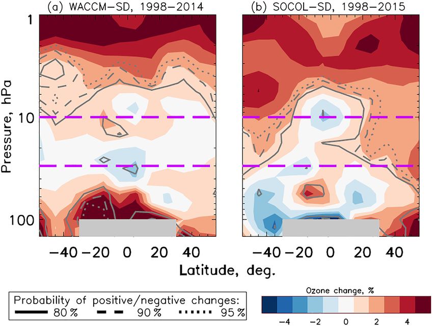
Figure 5. As for Fig. 1 but for (a) WACCM-SD and (b) SOCOL- in the upper stratosphere above 10 hPa, roughly in line with
SD. the observations (Fig. 1). Spatially, in the middle stratosphere
there are differences in sign, but generally significance is
low: WACCM-SD displays broadly positive changes except
A deeper investigation is needed to understand the contri- in the tropics at 10 and 30 hPa, SOCOL-SD displays a neg-
butions of tropospheric column ozone and stratospheric col- ative spot centred in the tropics at 10 hPa, and mid-latitudes
umn ozone to total column ozone, especially considering un- are often positive and significant. In the lower stratosphere,
certainties carefully, but this is beyond the scope of this work. SOCOL-SD displays negative trends in the Southern Hemi-
We note that studies using various data sources show less sig- sphere lower stratosphere but positive trends in the North-
nificant regional increases (and some decreases), with global ern Hemisphere, while WACCM-SD is generally positive ev-
estimates ranging from 0.2 to 0.7 % per year (∼ 0.6–2 DU per erywhere and significant at the lowest altitudes, except at
decade) (Cooper et al., 2014; Ebojie et al., 2016; Heue et al., 30–40 hPa in the tropics where a negative tendency is seen.
2016), though these estimates considered different time peri- In both SOCOL-SD and WACCM-SD, trends in the lower
ods. This suggests a large range of uncertainty, but even the stratosphere are generally not significant and do not display
lower end of the estimated increases in tropospheric column the clear and significant decreases found in the observations.
ozone are in line with the missing part of the total column Posterior distributions similar to those of Fig. 2 are presented
ozone change, after considering stratospheric column ozone for SOCOL-SD and WACCM-SD in Figs. S9 and S10, re-
that we estimate here. Tropospheric ozone is not the main spectively. The displayed behaviour is spatially similar to
focus of the study here, but the evidence presented overall that described here for the models in Fig. 5, and no significant
suggests that the missing component in the declining strato- decreases are found (two SOCOL-SD latitude bands display
spheric column ozone distributions and trends, with respect negative changes in the lower stratosphere with ∼ 75 % prob-
to constant total column ozone, is indeed from increasing tro- ability: 30–40◦ S and 10–20◦ N). It is worth noting that in
pospheric ozone. both cases the integrated, 60◦ S–60◦ N, trends in the strato-
spheric column ozone and upper stratosphere are all pos-
4.4 Comparison of stratospheric spatial and partial itive with probabilities of an increase exceeding 95 % and
column ozone trends with models positive in the lower stratosphere, with 69 and 85 % prob-
ability of an increase in SOCOL-SD and WACCM-SD, re-
The observational results for the lower, and whole, strato- spectively. The non-linear DLM trends (Fig. 3) of WACCM-
sphere presented thus far have not been previously reported. SD (blue) and SOCOL-SD (purple) emphasise the behaviour
However, it is not clear that this represents a departure from clearly differs from the observations, especially in the lower
our understanding of stratospheric trends as presented in stratosphere (the deseasonalised and regression model time
modelling studies. We present the percentage ozone change series are omitted from Fig. 3 for clarity but are provided
from two state-of-the-art CCMs in Fig. 5: (a) the NCAR
Community Earth System Model (CESM) Whole Atmo- 6 Use of MERRA-2 reanalysis (Gelaro et al., 2017) makes little
sphere Community Climate Model-4 (WACCM; Marsh et al., difference, except in the upper stratosphere after 2004, where pos-
2013) and (b) the SOlar Climate Ozone Links (SOCOL; itive trends are larger when using MERRA-2 (see Fig. S12). The
Stenke et al., 2013) model. Both simulations were performed WACCM-SD run with MERRA-2 uses CESM 1.2.2 at 1.9 × 2.5
with the Chemistry Climate Model Initiative phase 1 (CCMI- horizontal resolution and 88 vertical layers up to 140 km, using pre-
1) boundary conditions in specified dynamics (SD) mode scribed aerosols from the RCP8.5 scenario.
Atmos. Chem. Phys., 18, 1379–1394, 2018 www.atmos-chem-phys.net/18/1379/2018/W. T. Ball et al.: Continuous stratospheric ozone decline 1389
in Fig. S11). It is worth mentioning that the behaviour of iii. The main stratospheric dataset considered indicates a
stratospheric column ozone from the models was similar to highly probable (95 %) decrease in the ozone layer since
SBUV total column ozone (Fig. 3a) until around 2012, after 1998, i.e. in stratospheric ozone (between 147 and 1 hPa
which modelled ozone continued to increase while observa- (13–48 km) at mid-latitudes, or 100 and 1 hPa (17–
tions show a gradual decline until 2016 (see discussion in 48 km) at tropical latitudes) integrated over latitudes
Sect. 4.2). 60◦ S–60◦ N – the other composites support this result
The CCMVal-2 (SPARC, 2010) multi-model-mean 2000– when considering the associated caveats of each.
2013 ozone changes in the WMO (2014) ozone assessment
(chap. 2, Fig. 10) show a positive, but insignificant, change iv. There is no significant change in total column ozone
in the lower stratosphere at mid-latitudes, which suggests between 1998 and 2016, which includes both tropo-
models may not be simulating that region correctly, consis- spheric ozone and the stratospheric ozone layer – indeed
tent with the two models ending in 2014–2015. While CCMs no change is the most probable result indicated, which
capture historical ozone behaviour in the upper stratosphere our findings imply is a consequence of increasing tropo-
well, it is less clear in the UTLS region. Fig. 7.27–7.28 of the spheric ozone, together with the slowed rate of decrease
SPARC (2010) report indicate large differences compared to in stratospheric ozone following the Montreal Protocol.
observations in winter–spring, perhaps related to factors af- v. State-of-the-art models, nudged to have historical at-
fecting model transport (e.g. resolution, and gravity wave mospheric dynamics as realistic as possible, do not re-
parameterisations). Whether these differences result from produce these observed decreases in lower stratospheric
model design, incorrect boundary conditions (e.g. underes- ozone.
timated anthropogenic (Yu et al., 2017) or volcanic (Bandoro
et al., 2018) aerosol contributions), or missing chemistry re- We posit several possible explanations for the continuing
mains an open question. decline in lower stratospheric ozone, beginning with those
related to dynamics. First, part of the tropical and subtrop-
ical (< 30◦ ) lower stratospheric decline may be linked to a
5 Conclusions greenhouse-gas-related BDC acceleration (Randel and Wu,
2007; Oman et al., 2010; WMO, 2014) indicated from CCM
Following the successful implementation of the Montreal simulations, although observational evidence remains weak,
Protocol, total column ozone stabilised at the end of the and a faster BDC in general would slow ozone destruc-
1990s, but the search for the first signs of recovery in total tion cycles and hence mid-latitude ozone would increase
column ozone integrated between 60◦ S and 60◦ N have not and overcompensate for the tropical ozone reduction (WMO,
yet been successful (Weber et al., 2017; Chipperfield et al., 2014). Second, a rise in the tropopause (Santer et al., 2003),
2017). The lower stratosphere, below 24 km (∼ 32 hPa), con- due to the warming troposphere, could lead to a decrease
tains a large fraction of the total column ozone and is a re- in ozone at mid-latitudes (Steinbrecht et al., 1998; Varot-
gion of large natural variability that has previously inhibited sos et al., 2004), but the tropopause rise is also affected
detection of significant trends (Weatherhead and Andersen, by the ozone loss itself (Son et al., 2009), rendering its at-
2006). With longer time series, improved composites, and tribution difficult. Third, here we hypothesise a so-far-not-
integration of the lower stratospheric column, we can now discussed mechanism: an acceleration of the lower strato-
detect statistically significant trends in this region. We find sphere BDC shallow branch (Randel and Wu, 2007; Oman
that the negative ozone trend within the lower stratosphere et al., 2010) might increase transport of ozone-poor air to the
between 1998 and 2016 is the main reason why a statistically mid-latitudes from the tropical lower stratosphere (Johnston,
significant recovery in total column ozone has remained elu- 1975; Perliski et al., 1989). The quality of the applied dy-
sive. Our main findings are as follows: namical fields in the specified dynamics models considered
in this study, or the way models handle transport in the lower
i. We further confirm other studies that the Montreal Pro- stratosphere (SPARC, 2010; Dietmüller et al., 2017), may be
tocol is successfully reducing the impact of halogenated dynamically related reasons why models do not reproduce
ozone-depleting substances as indicated by the highly the observed lower stratospheric ozone changes.
probable recovery (> 95 %) measured in upper strato- While dynamically driven explanations may be fully re-
spheric regions (1–10 hPa or 32–48 km). sponsible for tropical lower stratospheric ozone changes,
at mid-latitudes additional chemically driven contributions
ii. Lower stratospheric ozone (between 147 and 32 hPa
from increasing anthropogenic and natural very-short-lived
(13–24 km) at mid-latitudes, or 100 and 32 hPa (17–
substances (VSLSs) containing chlorine or bromine may
24 km) at tropical latitudes) has continued to decrease
play a role (Hossaini et al., 2015). Modelling studies imply
since 1998 between 60◦ S and 60◦ N, with a probability
that VSLSs preferentially destroy lower stratospheric ozone,
of 99 % in two of the three analysed datasets and 87 %
though the effect outside of the polar latitudes is expected
in the third.
to be small (Hossaini et al., 2015, 2017). While VSLSs are
www.atmos-chem-phys.net/18/1379/2018/ Atmos. Chem. Phys., 18, 1379–1394, 20181390 W. T. Ball et al.: Continuous stratospheric ozone decline
thought to delay the recovery of the ozone layer, much un- W.: High solar cycle spectral variations inconsistent with
certainty remains since observations and reaction rate kinet- stratospheric ozone observations, Nat. Geosci., 9, 206–209,
ics are only available for some VSLSs (Oram et al., 2017). https://doi.org/10.1038/ngeo2640, 2016.
The uncertainties in model chemical boundary conditions, Ball, W. T., Alsing, J., Mortlock, D. J., Rozanov, E. V., Tum-
e.g. the prescribed emissions of VSLSs, therefore, may also mon, F., and Haigh, J. D.: Reconciling differences in strato-
spheric ozone composites, Atmos. Chem. Phys., 17, 12269–
be a reason why models do not reproduce the trends we re-
12302, https://doi.org/10.5194/acp-17-12269-2017, 2017.
port here. Bandoro, J., Solomon, S., Santer, B. D., Kinnison, D. E., and Mills,
The Montreal Protocol is working, but if the negative trend M. J.: Detectability of the impacts of ozone-depleting substances
in lower stratospheric ozone persists, its efficiency might be and greenhouse gases upon stratospheric ozone accounting for
disputed. Restoration of the ozone layer is essential to re- nonlinearities in historical forcings, Atmos. Chem. Phys., 18,
duce the harmful effects of solar UV radiation (WMO, 2014) 143–166, https://doi.org/10.5194/acp-18-143-2018, 2018.
that impact human and ecosystem health (Slaper et al., 1996). Bourassa, A. E., Degenstein, D. A., Randel, W. J., Zawodny, J.
Presently, models do not robustly reproduce the decline in M., Kyrölä, E., McLinden, C. A., Sioris, C. E., and Roth, C. Z.:
lower stratospheric ozone identified here. This will be imper- Trends in stratospheric ozone derived from merged SAGE II and
ative, both to predict future changes and to determine if it is Odin-OSIRIS satellite observations, Atmos. Chem. Phys., 14,
possible to prevent further decreases. 6983–6994, https://doi.org/10.5194/acp-14-6983-2014, 2014.
Bourassa, A. E., Roth, C. Z., Zawada, D. J., Rieger, L. A., McLin-
den, C. A., and Degenstein, D. A.: Drift corrected Odin-OSIRIS
ozone product: algorithm and updated stratospheric ozone trends,
Data availability. Merged-SWOOSH/GOZCARDS and Merged-
Atmos. Meas. Tech. Discuss., https://doi.org/10.5194/amt-2017-
SBUV, named “BASICSG ” and “BASICSBUV ” following the merg-
229, in review, 2017.
ing method used from Ball et al. (2017), are available for down-
Chehade, W., Weber, M., and Burrows, J. P.: Total ozone
load from https://data.mendeley.com/datasets/2mgx2xzzpk/2 (Als-
trends and variability during 1979–2012 from merged data
ing and Ball, 2017).
sets of various satellites, Atmos. Chem. Phys., 14, 7059–7074,
https://doi.org/10.5194/acp-14-7059-2014, 2014.
Chiodo, G., Marsh, D. R., Garcia-Herrera, R., Calvo, N., and
The Supplement related to this article is available online García, J. A.: On the detection of the solar signal in the
at https://doi.org/10.5194/acp-18-1379-2018-supplement. tropical stratosphere, Atmos. Chem. Phys., 14, 5251–5269,
https://doi.org/10.5194/acp-14-5251-2014, 2014.
Chipperfield, M. P., Bekki, S., Dhomse, S., Harris, N. R. P., Hassler,
B., Hossaini, R., Steinbrecht, W., Thiéblemont, R., and Weber,
M.: Detecting recovery of the stratospheric ozone layer, Nature,
Competing interests. The authors declare that they have no conflict 549, 211–218, https://doi.org/10.1038/nature23681, 2017.
of interest. Cooper, O. R., Parrish, D. D., Ziemke, J., Balashov, N. V., Cu-
peiro, M., Galbally, I. E., Gilge, S., Horowitz, L., Jensen,
N. R., Lamarque, J.-F., Naik, V., Oltmans, S. J., J., S.,
Acknowledgements. William T. Ball and Eugene V. Rozanov T., S. D., Thompson, A. M., Thouret, V., Wang, Y., and
were funded by the SNSF project 163206 (SIMA). We thank the Zbinden, R. M.: Global distribution and trends of tropospheric
SPARC LOTUS working group for discussion and data exchange. ozone: An observation-based review, Elem Sci Anth., p. 29,
Work at the Jet Propulsion Laboratory was performed under https://doi.org/10.12952/journal.elementa.000029, 2014.
contract with the National Aeronautics and Space Administration. Damadeo, R. P., Zawodny, J. M., and Thomason, L. W.: Reeval-
GOZCARDS ozone data contributions from Ryan Fuller (at JPL) uation of stratospheric ozone trends from SAGE II data using
are gratefully acknowledged. We are grateful to Daniel Marsh and a simultaneous temporal and spatial analysis, Atmos. Chem.
Doug Kinnison for providing ozone data from WACCM CESM in Phys., 14, 13455–13470, https://doi.org/10.5194/acp-14-13455-
specified dynamics mode. 2014, 2014.
Davis, S. M., Rosenlof, K. H., Hassler, B., Hurst, D. F., Read,
Edited by: Marc von Hobe W. G., Vömel, H., Selkirk, H., Fujiwara, M., and Damadeo,
Reviewed by: two anonymous referees R.: The Stratospheric Water and Ozone Satellite Homogenized
(SWOOSH) database: a long-term database for climate studies,
Earth Syst. Sci. Data, 8, 461–490, https://doi.org/10.5194/essd-
8-461-2016, 2016.
References Dee, D. P., Uppala, S. M., Simmons, A. J., Berrisford, P., Poli,
P., Kobayashi, S., Andrae, U., Balmaseda, M. A., Balsamo, G.,
Alsing, J. and Ball, W. T.: BASIC-SG (Merged-SWOOSH- Bauer, P., Bechtold, P., Beljaars, A. C. M., van de Berg, L., Bid-
GOZCARDS) for “Evidence for a continuous decline in lot, J., Bormann, N., Delsol, C., Dragani, R., Fuentes, M., Geer,
lower stratospheric ozone offsetting ozone layer recovery”, A. J., Haimberger, L., Healy, S. B., Hersbach, H., Hólm, E. V.,
https://doi.org/10.17632/2mgx2xzzpk.1, 2017. Isaksen, L., Kållberg, P., Köhler, M., Matricardi, M., McNally,
Ball, W. T., Haigh, J. D., Rozanov, E. V., Kuchar, A., A. P., Monge-Sanz, B. M., Morcrette, J.-J., Park, B.-K., Peubey,
Sukhodolov, T., Tummon, F., Shapiro, A. V., and Schmutz,
Atmos. Chem. Phys., 18, 1379–1394, 2018 www.atmos-chem-phys.net/18/1379/2018/You can also read