Differences in the quasi-biennial oscillation response to stratospheric aerosol modification depending on injection strategy and species
←
→
Page content transcription
If your browser does not render page correctly, please read the page content below
Atmos. Chem. Phys., 21, 8615–8635, 2021
https://doi.org/10.5194/acp-21-8615-2021
© Author(s) 2021. This work is distributed under
the Creative Commons Attribution 4.0 License.

Differences in the quasi-biennial oscillation response to stratospheric
aerosol modification depending on injection strategy and species
Henning Franke1,2 , Ulrike Niemeier1 , and Daniele Visioni3
1 Max  Planck Institute for Meteorology, Bundesstr. 53, 20146 Hamburg, Germany
2 InternationalMax Planck Research School on Earth System Modelling, Bundesstr. 53, 20146 Hamburg, Germany
3 Sibley School for Mechanical and Aerospace Engineering, Cornell University, Ithaca, NY, USA

Correspondence: Henning Franke (henning.franke@mpimet.mpg.de)

Received: 22 October 2020 – Discussion started: 6 November 2020
Revised: 5 February 2021 – Accepted: 3 May 2021 – Published: 8 June 2021

Abstract. A known adverse side effect of stratospheric              1   Introduction
aerosol modification (SAM) is the alteration of the quasi-
biennial oscillation (QBO), which is caused by the strato-
spheric heating associated with an artificial aerosol layer.        Stratospheric aerosol modification (SAM) by the artificial in-
Multiple studies found the QBO to slow down or even com-            jection of sulfur dioxide (SO2 ) into the lower stratosphere
pletely vanish for point-like injections of SO2 at the Equa-        is currently widely discussed as a potential measure against
tor. The cause for this was found to be a modification of           global warming for the case of unmitigated greenhouse gas
the thermal wind balance and a stronger tropical upwelling.         (GHG) emissions. It would basically mimic the processes af-
For other injection strategies, different responses of the QBO      ter a large stratospheric volcanic eruption, resulting in an en-
have been observed. A theory which is able to explain those         hancement of the natural stratospheric sulfate aerosol layer.
differences in a comprehensive manner has not yet been pre-         Since sulfate aerosols backscatter incoming shortwave ra-
sented. This is further complicated by the fact that the sim-       diation (ISR), this enhancement of the stratospheric sulfate
ulated QBO response is highly sensitive to the used model           aerosol layer causes a negative radiative forcing (RF) on
even under identical boundary conditions. Therefore, within         the Earth system, which would counteract the tropospheric
this study we investigate the response of the QBO to SAM            warming caused by increasing atmospheric GHG concentra-
for three different injection strategies (point-like injection at   tions.
the Equator, point-like injection at 30◦ N and 30◦ S simulta-          Besides backscattering ISR, sulfate aerosols also ab-
neously, and areal injection into a 60◦ wide belt along the         sorb parts of the outgoing tropospheric longwave radiation
Equator). Our simulations confirm that the QBO response             (OTLR) and the incoming near-infrared radiation (NIRR).
significantly depends on the injection location. Based on the       The absorption of OTLR and NIRR causes a significant
thermal wind balance, we demonstrate that this dependency           warming of the lower tropical stratosphere (e.g., Heckendorn
is explained by differences in the meridional structure of the      et al., 2009; Ferraro et al., 2011). This warming has im-
aerosol-induced stratospheric warming, i.e., the location and       portant consequences for stratospheric dynamics, including
meridional extension of the maximum warming. Addition-              the quasi-biennial oscillation (QBO). The QBO is a zon-
ally, we also tested two different injection species (SO2 and       ally symmetric oscillation of the zonal wind in the trop-
H2 SO4 ). The QBO response is qualitatively similar for both        ical stratosphere with an average period of approximately
investigated injection species. Comparing the results to cor-       28 months (Baldwin et al., 2001; Naujokat, 1986). It is char-
responding results of a second model, we further demonstrate        acterized by an alternating downwelling of westerly and east-
the generality of our theory as well as the importance of an        erly winds from the upper stratosphere, above 5 hPa, into the
interactive treatment of stratospheric ozone for the simulated      tropopause region, where these wind patterns are rapidly at-
QBO response.                                                       tenuated (Baldwin et al., 2001; Holton, 2004). The QBO has
                                                                    an impact on tropospheric winds (Garfinkel and Hartmann,

Published by Copernicus Publications on behalf of the European Geosciences Union.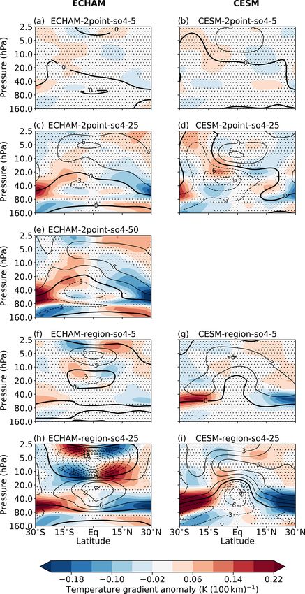
8616                            H. Franke et al.: Quasi-biennial oscillation response to stratospheric aerosol modification

2011) and precipitation (Seo et al., 2013), as well as on the      dent in a simulation without SAM, as the main cause of dif-
stratospheric transport to the extratropics (Plumb and Bell,       ferences. Since the models used in the aforementioned stud-
1982; Punge et al., 2009) and the polar vortex (Holton and         ies as well as their specific setup vary significantly, the com-
Tan, 1980). After the major eruption of Mt. Pinatubo in June       parability of their results is consequently reduced. This fur-
1991, the lower stratosphere warmed by about 3 K, which led        ther complicates the search for a comprehensive explanation
to a prolonged QBO westerly phase in the lower stratosphere        of the at least partly contradictory QBO response to different
(Labitzke, 1994), very likely due to an increased tropical up-     injection locations.
welling induced by the aerosol warming (Giorgetta et al.,             To overcome this limitation, in this study we investigate
2011, Henning Franke and Marco Giorgetta, personal com-            the QBO response to three different injection locations for
munication, 2020).                                                 the same models as used by Niemeier et al. (2020) but with
   Multiple studies revealed that the QBO could also be heav-      a different model setup in one case (see model description
ily perturbed during a potential deployment of SAM (e.g.,          in Sect. 2). Both models followed the experimental protocol
Aquila et al., 2014; Richter et al., 2017; Tilmes et al., 2018;    of the GeoMIP6 test bed experiment accumH2SO4 (Weisen-
Niemeier et al., 2020). For equatorial point injections, Aquila    stein and Keith, 2018) to compare the different efficiencies
et al. (2014) obtained a prolonged or even permanent QBO           of SO2 and H2 SO4 . Since multiple studies found that the
westerly phase, depending on the injection rate. They at-          forcing efficiency decreases significantly with increasing in-
tributed these modifications of the QBO basically to two           jection rates of SO2 (e.g., Heckendorn et al., 2009; English
physical mechanisms: a modification of the thermal wind            et al., 2012; Niemeier and Timmreck, 2015; Vattioni et al.,
balance due to the aerosol-induced warming of the lower            2019), the direct injection of gaseous H2 SO4 instead of SO2
tropical stratosphere and an acceleration of the tropical up-      has been suggested as a potential alternative (Pierce et al.,
welling as a response to this warming, which decelerates the       2010; Benduhn et al., 2016). For both models, we tested an
downward propagation of the QBO. Niemeier and Schmidt              injection into a zonal belt along the Equator ranging from
(2017) and Richter et al. (2017) further confirmed these re-       30◦ N to 30◦ S and a simultaneous point-like injection at
sults with other models.                                           30◦ N and 30◦ S, and for one model we additionally tested
   Together with equatorial point injections, a modification       an equatorial point injection. Unlike previous studies, we aim
of the QBO has been also noticed for other injection strate-       for an advanced understanding of the dynamical mechanisms
gies. Niemeier and Schmidt (2017) obtained a significantly         which lead to the SAM-induced modification of the QBO for
prolonged westerly phase of the QBO for an injection into          different injection locations. We will in particular focus on
a zonal belt along the Equator ranging from 30◦ N to 30◦ S         the modification of thermal wind balance by explicitly study-
with an injection rate of 10 Tg(S) yr−1 but weaker than for        ing the SAM-induced modification of the meridional temper-
an equatorial point injection with the same injection rate. For    ature gradient within the stratosphere, which was not done so
point-like injections in the extratropics, the QBO response        far.
to SAM is also different. Richter et al. (2017) showed that           In Sect. 2, the models used in this study as well as the per-
the QBO speeds up instead of slowing down for point-like           formed simulations are described. The results are structured
injections at 15◦ N, 15◦ S, 30◦ N, and 30◦ S, testing an in-       as follows. In Sect. 3, we investigate the dependency of the
jection rate of 6 Tg(S) yr−1 . The root cause of this acceler-     QBO response to the injection location, rate, and species in
ation was not finally determined, despite a detailed analysis      our first model (MAECHAM5-HAM). Thereby, we give the
of the 2◦ N–2◦ S zonal mean momentum budget. Tilmes et al.         theoretical explanation of the different responses to SAM –
(2018) analyzed a simultaneous injection at two points at          focusing on the modification of thermal wind balance – in
15◦ N and 15◦ S for two different injection heights with injec-    Sect. 3.1.3. In Sect. 4, we then compare the SAM-induced
tion rates of 12 and 16 Tg(S) yr−1 . Within their simulations,     modification of the QBO observed in MAECHAM5-HAM
the QBO slightly slows down but with a prolonged easterly          to that observed in CESM2(WACCM). This study ends with
phase within the lower stratosphere instead of a prolonged         a discussion and a conclusion of the main findings in Sect. 5.
westerly phase as for equatorial point injections. They argue
that the short simulation period and the low vertical resolu-
tion of their model may be a reason for these contradictory        2     Model and setup of the simulations
results.
   Additionally, Niemeier et al. (2020) showed that the sim-       2.1    MAECHAM5-HAM
ulated QBO response to SAM may be very sensitive to the
used model itself by comparing two models (MAECHAM5-               MAECHAM5 is the middle atmosphere version of the spec-
HAM and WACCM-110L) using the same model setup and                 tral general circulation model (GCM) ECHAM5 (Roeckner
injection protocol. Both models showed a qualitatively sim-        et al., 2003; Giorgetta et al., 2006; Roeckner et al., 2006).
ilar QBO response to SAM but quantitatively much stronger          It simulates the evolution of atmospheric dynamics by nu-
in WACCM-110L. The authors assumed differences in the              merically solving prognostic equations for temperature, sur-
vertical residual velocities in the tropics, which are also evi-   face pressure, vorticity, and divergence in terms of spherical

Atmos. Chem. Phys., 21, 8615–8635, 2021                                              https://doi.org/10.5194/acp-21-8615-2021
H. Franke et al.: Quasi-biennial oscillation response to stratospheric aerosol modification                                8617

harmonics. The different phases of water as well as tracers       dle atmospheric (stratosphere, mesosphere and lower ther-
are transported within the model using a flux-form semi-          mosphere) chemistry, with 98 simulated chemical species.
Lagrangian transport scheme (Lin and Rood, 1996). De-             Sulfate aerosols are treated using the Modal Aerosol Model
tails on ECHAM5 can be found in Roeckner et al. (2003).           (MAM4) as described in Liu et al. (2012, 2016) but with
MAECHAM5 has a vertical domain which extends from the             some modifications to change the mode widths and to the
surface up to 0.01 hPa while being resolved by 90 sigma-          capabilities of sulfate aerosol to grow into the larger mode;
pressure levels. Additionally, it accounts for the momentum       an explanation of this and an evaluation of its capabilities in
flux deposition of unresolved gravity waves (GWs) originat-       simulating volcanic aerosols after Pinatubo is given in Mills
ing from the troposphere via a parameterization following         et al. (2016, 2017). CESM2(WACCM) will be hereafter re-
Hines (1997a, b); its implementation into MAECHAM5 is             ferred to as CESM.
described by Manzini et al. (2006). Therefore, MAECHAM5
internally generates a QBO in the tropical stratosphere (Gior-    2.3   Simulations
getta et al., 2006). For this study, MAECHAM5 was used
with a spectral truncation at wave number 42 (T42), result-       The experimental setup of the simulations performed in this
ing in a horizontal Gaussian grid with 64 × 128 grid boxes        study is in accordance with the proposal of the GeoMIP6
with a size of 2.8◦ × 2.8◦ per grid box.                          test bed experiment accumH2SO4 (Weisenstein and Keith,
   MAECHAM5 was interactively coupled to the prognos-             2018) for both models. In all simulations, the sea surface
tic modal aerosol microphysical model HAM (Stier et al.,          temperature (SST) and the sea ice concentration (SIC) were
2005), which is based on the microphysical core M7 devel-         set to monthly climatological values of the period 1988 to
oped by Vignati et al. (2004). HAM calculates aerosol mi-         2007 out of the AMIP SST data set following the experi-
crophysical processes like nucleation, accumulation, conden-      mental setup in Butchart et al. (2018). The GHG concentra-
sation, and coagulation as well as the sulfate aerosol deple-     tions and the concentrations of ozone-depleting substances
tion via sedimentation and deposition (Stier et al., 2005). In    (ODSs) are taken from the SSP5-8.5 scenario of Scenari-
this setup of HAM, a simple stratospheric sulfur chemistry        oMIP (O’Neill et al., 2016) for the year 2040. This combi-
is applied in the stratosphere, which uses prescribed monthly     nation of GHG and SST forcing allows us to approximately
oxidant fields and photolysis rates of, inter alia, ozone, OH,    mimic the surface cooling that would be produced by the
and NOx (Timmreck, 2001; Hommel and Graf, 2011). There-           sulfate layer, while having a consistent surface field for all
fore, the impact of SAM on stratospheric ozone is not sim-        models and thus removing the source of uncertainty derived
ulated within MAECHAM5-HAM. Within this stratospheric             from differences in the simulated cooling amongst models.
HAM version, apart from the injected SO2 or H2 SO4 , only         Due to their coarse horizontal resolution, the used models
natural sulfur emissions are taken into account. These sim-       are not able to simulate the rapid initial formation of accu-
ulations use the model setup described in Niemeier et al.         mulation mode sulfate particles (AM−SO4 ) after the injec-
(2009) and Niemeier and Timmreck (2015), where more de-           tion of H2 SO4 . Therefore, the injection of H2 SO4 is mod-
tails can be found. The HAM aerosol model couples back to         eled as a direct injection of an AM−SO4 population with a
the dynamics by the aerosol optical properties in the short-      mode radius of 0.075 µm and a standard deviation of 1.59
wave, longwave, and near-infrared range, which enter the ra-      in ECHAM and a mode radius of 0.1 µm and a standard de-
diative transfer scheme in MAECHAM5 and thus influence            viation of 1.5 in CESM, both following the proposal of ac-
the temperature. Consequently, the interactive modification       cumH2SO4 (Weisenstein and Keith, 2018).
of the QBO is simulated within MAECHAM5-HAM, which                   With ECHAM, three different injection strategies have
will be hereafter referred to as ECHAM.                           been simulated for both injection species (SO2 and
                                                                  AM−SO4 ): an injection into one single grid box centered
2.2   CESM2(WACCM)                                                at 1.4◦ N, 180◦ E (termed point); a simultaneous injection
                                                                  into two grid boxes centered at 29.3◦ N, 180◦ E and 29.3◦ S,
The Community Earth System Model version 2 (release 2.1)          180◦ E (termed 2point); and an injection into a zonally sym-
in the Whole Atmosphere Community Climate Model ver-              metric belt from 30◦ N to 30◦ S along the Equator (termed
sion CESM2(WACCM6) is a state-of-the-art fully coupled            region). The injections took place in three adjacent model
climate model, which is also used in the new CMIP6 simu-          layers at a height between 18 and 20 km. With CESM, only
lations (Gettelman et al., 2019). It uses 72 vertical layers up   the 2point and region injections have been simulated. The
to about 150 km and a 0.9◦ in latitude by 1.25◦ in longitude      point injection strategy is not part of the accumH2SO4 ex-
horizontal grid. WACCM6 includes convective, frontal, and         perimental protocol and was, therefore, not performed by
orographic sources of GWs, which propagate to drive the cir-      CESM. For the 2point injections, the injections took place
culation of the middle atmosphere, including the QBO.             in a single model layer at 20 km, while for the region in-
   Although the standard version of WACCM6 uses com-              jections the injections took place between 19 and 21 km. All
prehensive chemistry from the troposphere to the lower            injection scenarios have been simulated with two different in-
thermosphere, the version used here only simulates mid-           jection rates for both models: 5 and 25 Tg(S) yr−1 , as given

https://doi.org/10.5194/acp-21-8615-2021                                           Atmos. Chem. Phys., 21, 8615–8635, 2021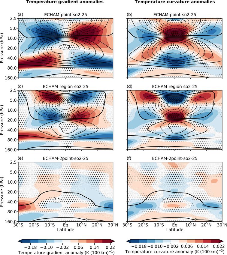
8618 H. Franke et al.: Quasi-biennial oscillation response to stratospheric aerosol modification
by the accumH2SO4 protocol. The injection rate is the to- strength of the QBO modification does not show a significant
tal amount of sulfur that is injected globally per year; for dependence on the injection species in our simulations.
example, in the 2point injections with an injection rate of
25 Tg(S) yr−1 , both injection points have an injection rate of 3.1 Dynamic mechanisms of QBO modification
12.5 Tg(S) yr−1 . For the 2point injection of AM−SO4 with
ECHAM, an additional simulation with an injection rate of The dynamic mechanisms which cause the observed modifi-
50 Tg(S) yr−1 has been performed. An overview of all per- cation and breakdown of the QBO for an equatorial point in-
formed simulations and their setups can be found in Table 1. jection of SO2 have been investigated by Aquila et al. (2014).
All simulations were performed for a period of 10 years. They argue that the absorption of radiation in the near IR and
If not otherwise stated, the results presented in this study are terrestrial wavelengths by the artificial sulfate aerosols and
averaged over the last 8 years of the respective simulation, the associated lower-stratospheric heating are the root cause
since Visioni et al. (2019) showed that the artificial strato- of the observed changes in QBO dynamics. In more detail,
spheric sulfate layer has reached equilibrium already by the they identified that this aerosol-induced warming modifies
third year of deployment. All anomalies presented in this thermal wind balance in the lower tropical stratosphere and
study have been calculated with respect to the control sim- increases the residual tropical upwelling in the rising branch
ulation (termed contr-000) of the corresponding model. The of the Brewer–Dobson circulation (BDC), both causing a
control simulations were performed with the same SST, SIC, modification of the QBO.
GHG, and ODS specifications like the SAM simulations but In this section, we will investigate the reasons for the dif-
without any artificial injection of some sulfur species. ferent QBO responses to the three tested injection strategies
exemplarily based on an injection of SO2 with an injection
rate of 25 Tg(S) yr−1 (experiments point-so2-25, region-so2-
3 QBO response to SAM in ECHAM 25, 2point-so2-25). This injection scenario follows the ex-
perimental setup of Aquila et al. (2014) with regard to the
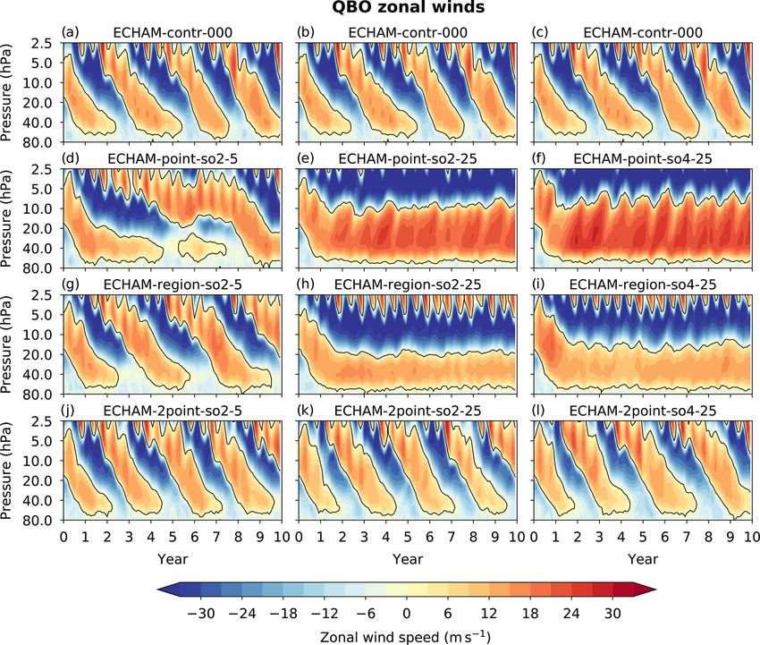
ECHAM simulates the QBO well in the control simulation injection type and has a high signal-to-noise ratio due to the
(Fig. 1a–c), where it has a period of roughly 32 months, high injection rate. The impact of a lower injection rate and
which is slightly longer than the observed period of approxi- another injection species (i.e., AM−SO4 instead of SO2 ) will
mately 28 months (Naujokat, 1986). Artificial sulfur injec- be discussed in Sect. 3.2 and 3.3.
tions may lead to a substantial modification of the QBO Additionally, we are aware of the fact that the QBO may
compared to the control simulation in ECHAM, depend- also change due to a modified wave driving. However, we
ing on the injection strategy, injection species, and injec- found no significant changes in QBO wave driving in our
tion rate (Fig. 1d–i). The equatorial point injections lead to simulations (not shown), which is in agreement with earlier
the most significant modification of the QBO compared to studies (e.g., Aquila et al., 2014; Richter et al., 2017; Tilmes
the other injection strategies: while an injection of SO2 with et al., 2018). Therefore, within this section we will only focus
an injection rate of 5 Tg(S) yr−1 (Fig. 1d) already leads to on the increase of the tropical upwelling and the modification
a drastic slowdown of the QBO with a prolonged lower- of thermal wind balance.
stratospheric westerly phase, the QBO is locked in a con-
stant lower-stratospheric westerly phase for a SO2 injection 3.1.1 Aerosol-induced heating of the lower stratosphere
with an injection rate of 25 Tg(S) yr−1 (Fig. 1e). On top of
the constant westerlies, constant easterlies are prevalent in The artificial sulfate aerosols heat the lower stratosphere by
the upper stratosphere. For the region injection of SO2 with the absorption of OTLR and NIRR, whereby the location and
an injection rate of 5 Tg(S) yr−1 (Fig. 1g), the period of the magnitude of this heating strongly correlate with those of the
QBO is clearly prolonged, and westerlies dominate in the sulfate mass mixing ratio mSO4 (Fig. 2a, c, e). For an equato-
lower stratosphere. For the region injection of SO2 with an rial point injection (Fig. 2a), the sulfate aerosols are strongly
injection rate of 25 Tg(S) yr−1 (Fig. 1h), the QBO is also concentrated within the tropics, which leads to a strong heat-
locked down in a permanent westerly phase but with weaker ing of the lower tropical stratosphere peaking at the Equator.
westerlies than for the corresponding point injection. In con- In contrast, the sulfate aerosols are distributed meridionally
trast to the point and region injections, the QBO is basically more uniform for the region injection and even more so for
not modified for the 2point injections of both tested injection the 2point injection (Fig. 2c, e), which also results in a merid-
rates in terms of periodicity and strength with respect to the ionally more uniform heating for the region and the 2point
control simulation (Fig. 1j, k). injection than for the point injection.
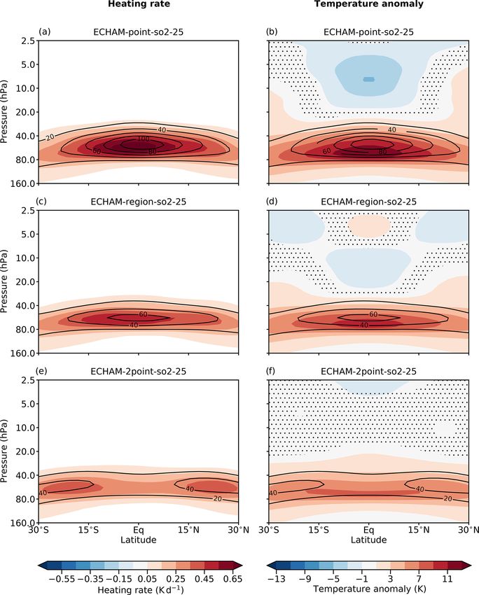
For an injection of AM−SO4 (Fig. 1 right column), the This aerosol-induced heating results in a significant posi-
modification of the QBO is slightly stronger than for the cor- tive temperature anomaly centered at the Equator (Fig. 2b, d,
responding injection of SO2 with the same injection strat- f). Following the meridional structure of the net aerosol heat-
egy and rate (Fig. 1 middle column) when using the point ing rates, the lower-stratospheric temperature anomaly has
and region injection strategies. For the 2point injections, the a clear equatorial peak for the point injection and its pole-
Atmos. Chem. Phys., 21, 8615–8635, 2021 https://doi.org/10.5194/acp-21-8615-2021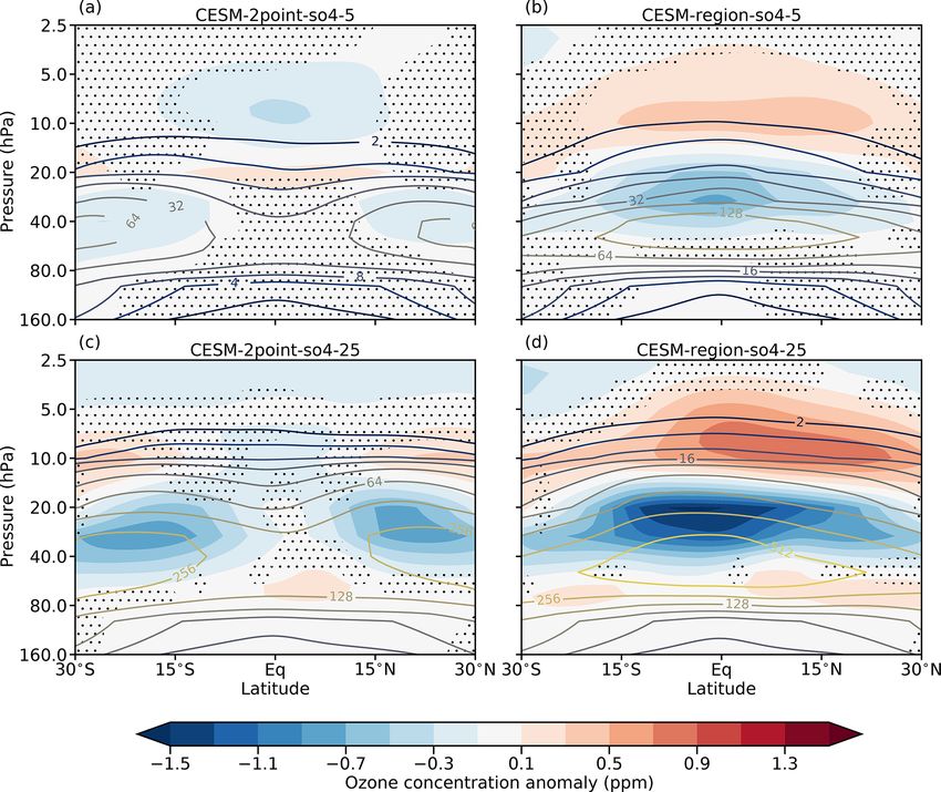
H. Franke et al.: Quasi-biennial oscillation response to stratospheric aerosol modification                                           8619

Table 1. Setup of all performed simulations. The point injections have been performed in a single equatorial grid box centered at 1.4◦ N,
180◦ E; the 2point injections have been performed in two boxes centered at 29.3◦ N, 180◦ E and 29.3◦ S, 180◦ E; and the region injections
have been performed in a belt along the whole Equator, ranging from 30◦ N to 30◦ S. The injection rate is the total amount of sulfur that is
injected globally per year. Check marks indicate whether the experiment was performed for the according model, while values in parenthesis
after the check marks indicate the injection altitude.

                Experiment       Injection species   Injection rate    Injection location   ECHAM            CESM
                contr-000        –                   –                 –                    X                X
                point-so2-5      SO2                 5 Tg(S) yr−1      equatorial box       X (18–20 km)     –
                point-so2-25     SO2                 25 Tg(S) yr−1     equatorial box       X (18–20 km)     –
                point-so4-5      AM−SO4              5 Tg(S) yr−1      equatorial box       X (18–20 km)     –
                point-so4-25     AM−SO4              25 Tg(S) yr−1     equatorial box       X (18–20 km)     –
                2point-so2-5     SO2                 5 Tg(S) yr−1      2 boxes              X (18–20 km)     X (20 km)
                2point-so2-25    SO2                 25 Tg(S) yr−1     2 boxes              X (18–20 km)     X (20 km)
                2point-so4-5     AM−SO4              5 Tg(S) yr−1      2 boxes              X (18–20 km)     X (20 km)
                2point-so4-25    AM−SO4              25 Tg(S) yr−1     2 boxes              X (18–20 km)     X (20 km)
                2point-so4-50    AM−SO4              50 Tg(S) yr−1     2 boxes              X (18–20 km)     –
                region-so2-5     SO2                 5 Tg(S) yr−1      30◦ N to 30◦ S       X (18–20 km)     X (19–21 km)
                region-so2-25    SO2                 25 Tg(S) yr−1     30◦ N to 30◦ S       X (18–20 km)     X (19–21 km)
                region-so4-5     AM−SO4              5 Tg(S) yr−1      30◦ N to 30◦ S       X (18–20 km)     X (19–21 km)
                region-so4-25    AM−SO4              25 Tg(S) yr−1     30◦ N to 30◦ S       X (18–20 km)     X (19–21 km)

ward gradients are sharp (Fig. 2b). For the region injection,           residual mean circulation. The residual mean circulation it-
the lower-stratospheric temperature anomaly still peaks at the          self may be described by the residual meridional and verti-
Equator but with a smaller absolute magnitude, leading to a             cal velocities v ∗ and w∗ , respectively, or by its mass stream
smaller poleward gradient (Fig. 2d). For the 2point injection,          function χ. For equatorial point injections of SO2 , Aquila
the temperature anomaly is meridionally nearly uniform be-              et al. (2014) showed that an aerosol-induced increase of w∗
tween 15◦ N and 15◦ S (Fig. 2f).                                        is associated with a stronger residual vertical advection of
   The warming of the lower stratosphere is the primary per-            zonal momentum (−w∗ uz ). A stronger −w∗ uz in the tropical
turbation induced by the sulfate aerosols, as indicated by              stratosphere weakens the downwelling of the QBO phases,
the good agreement of the sulfate mass mixing ratio, the                which leads to a prolongation of the QBO period.
net aerosol heating rates, and the temperature anomalies. All              Our simulations confirm that w ∗ increases statistically sig-
changes in dynamics – including the QBO – are obviously                 nificantly within the tropics for point-so2-25 and region-so2-
induced by this initial warming in a second step.                       25 and that this increase results in a stronger −w ∗ uz in the
   Opposite to the lower-stratospheric warming, statistically           upper tropical stratosphere (Fig. 3a, b). Thereby, the anoma-
significant negative temperature anomalies are located in the           lies are slightly stronger for point-so2-25 than for region-so2-
middle and upper tropical stratosphere for all three injec-             25 due to the stronger aerosol-induced stratospheric warm-
tion strategies (Fig. 2b, d, f). However, Fig. 2 clearly shows          ing. The maximum anomalies of w ∗ uz are located at the al-
that this cooling is not induced by the radiative effects of the        titudes of strongest easterly shear (see Fig. 1e, h). This in-
aerosols, as it is located well above the aerosol layer and does        dicates that the increase of the tropical upwelling helps to
not match with the net aerosol heating rates. Consequently,             maintain the permanent westerlies against the downwelling
these negative temperature anomalies have been induced dy-              easterlies aloft. For 2point-so2-25, w ∗ and −w∗ uz do not
namically due to an increased tropical upwelling (see Aquila            show a statistically significant increase throughout the whole
et al., 2014). Therefore, they cannot be seen as a root cause           tropical stratosphere (i.e., between 15◦ N and 15◦ S) (Fig. 3c).
of any change in the QBO.                                               The zonal mean residual circulation as a whole is also only
                                                                        weakly modified in the tropical stratosphere. This is in ac-
3.1.2   Modification of the residual circulation                        cordance with our observation that the amplitude and the pe-
                                                                        riodicity of the QBO basically remain unchanged for 2point-
Following Aquila et al. (2014), an increase of the tropical up-         so2-25 (Fig. 1k).
welling in the rising branch of the BDC due to the aerosol-                The reason for the increase of w∗ is the aerosol-induced
induced warming is the main reason for the modification of              stratospheric temperature anomaly, which alters the charac-
the QBO. Commonly, the BDC is treated in the so-called                  teristics of the zonal jets in the extratropical stratosphere.
transformed Eulerian mean (TEM) framework as outlined                   Thereby, the conditions for the vertical propagation of plan-
by Andrews et al. (1987), in which it is represented by the

https://doi.org/10.5194/acp-21-8615-2021                                                    Atmos. Chem. Phys., 21, 8615–8635, 2021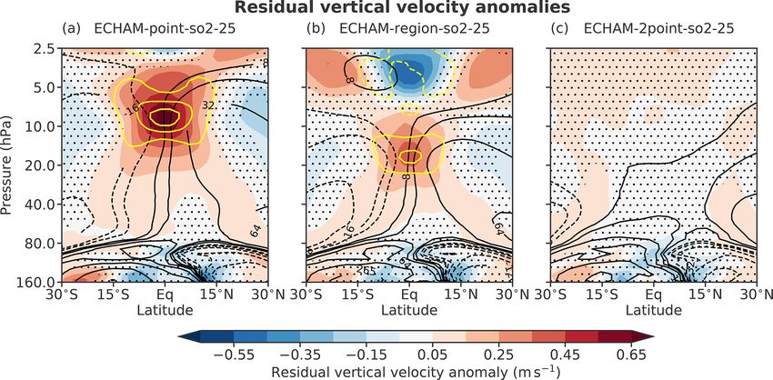
8620                               H. Franke et al.: Quasi-biennial oscillation response to stratospheric aerosol modification

Figure 1. Time–height cross sections of the 5◦ N to 5◦ S mean zonal wind in the stratosphere over the simulation period of 10 years for
ECHAM for different injection scenarios. The columns indicate the injection species and rate: the left column shows SO2 injections with
an injection rate of 5 Tg(S) yr−1 , the middle column shows SO2 injections with an injection rate of 25 Tg(S) yr−1 , and the right column
shows AM−SO4 injections with an injection rate of 25 Tg(S) yr−1 . The rows indicate the injection strategy: the first row shows the control
simulation, the second row shows the point injection, the third row shows the region injections, and the fourth row shows the 2point injection.
The solid black line marks a tropical mean zonal wind speed of 0 m s−1 .

etary waves in this region change. As a consequence, the ex-              tropical w ∗ increased by up to 100 % in the upper strato-
tratropical wave driving of the residual mean circulation in-             sphere (not shown). In contrast, in ECHAM simulations with
creases, which ultimately speeds up the whole BDC. This                   permanent lower-stratospheric easterlies instead of a QBO,
mechanism has been investigated by Tilmes et al. (2018) for               Niemeier et al. (2011) obtained an increase of the tropical w∗
SAM simulations and was also recognized in simulations of                 of only 5 % to 10 % for an equatorial point injection of SO2
a tropical volcanic eruption by Bittner et al. (2016).                    with an injection rate of 4 Tg(S) yr−1 . Therefore, one has to
   In the upper stratosphere (i.e., between 20 and 3 hPa                  be cautious when interpreting the strong positive anomalies
in point-so2-25 and between 25 and 8 hPa in region-so2-                   of −w∗ uz observed in the upper stratosphere in point-so2-25
25), this increase of w∗ is superimposed by changes in                    and region-so2-25 as the primary cause for the disruption of
the secondary meridional circulation (SMC) of the modified                the QBO since they are – at least partly – rather its conse-
QBO itself. During a permanent QBO westerly phase, the                    quence.
SMC would also be permanently locked in its corresponding                    Within the TEM framework, the characteristics of the gen-
“westerly” phase, which acts to increase w∗ within the trop-              eral acceleration of the BDC can be further directly linked to
ical stratosphere (Plumb and Bell, 1982). Our experiments                 the tropical confinement of the aerosol-induced temperature
indicate that a large fraction of the increase of w∗ in the up-           anomaly, as shown by Dunkerton (1983) in a study on the ef-
per tropical stratosphere (Fig. 3a, b) can be attributed to this          fect of the 1963 eruption of Mt. Agung on the QBO. Follow-
“indirect” acceleration via the SMC, especially in the upper              ing the equation of the residual mean meridional streamfunc-
stratosphere. For example, in the experiment point-so2-5, the             tion (Plumb and Bell, 1982), only a tropically confined heat-

Atmos. Chem. Phys., 21, 8615–8635, 2021                                                      https://doi.org/10.5194/acp-21-8615-2021
H. Franke et al.: Quasi-biennial oscillation response to stratospheric aerosol modification                                              8621

Figure 2. Latitude–height cross section of the zonal mean net aerosol heating rate (a, c, e) and of the anomaly of the zonal mean temperature
T (b, d, f) for the ECHAM simulations of point-so2-25 (a, b), region-so2-25 (c, d), and 2point-so2-25 (e, f). Stippling indicates areas where
the temperature anomalies are not significant at the 95 % level in Student’s t test. Black contour lines indicate the anomaly of the zonal mean
sulfate mass mixing ratio mSO4 in intervals of 20 µg(S) kg−1 .

ing modifies the BDC, whereas a meridionally uniform heat-                3.1.3   Modification of thermal wind balance
ing has no effect. This explains why the residual tropical up-
welling increases in point-so-25 and region-so2-25 but not in             Besides the increase of the tropical upwelling in the rising
2point-so2-25: while in point-so2-25 and region-so2-25 the                branch of BDC, Aquila et al. (2014) also attributed the ob-
aerosol heating has an equatorial peak and decreases rather               served changes in the QBO to a modification of thermal wind
sharply towards the extratropics, in 2point-so2-25 it is merid-           balance. Thermal wind balance is an atmospheric state equa-
ionally nearly uniform within the tropics (see Sect. 3.1.1).              tion, which links the zonal mean meridional temperature gra-
   Consequently, it is ultimately the meridional shape of the             dient T y to the zonal mean vertical wind shear uz . It is de-
aerosol-induced lower-stratospheric temperature anomaly or                fined as
– simply spoken – the degree of tropical confinement of the
                                                                          uz = −R(Hβy)−1 T y                                               (1)
artificial sulfate aerosols that determines the QBO response
to artificial sulfate injections.                                         for an equatorial β plane (Holton, 2004). Assuming equa-
                                                                          torial symmetry of the zonal mean temperature field, one

https://doi.org/10.5194/acp-21-8615-2021                                                    Atmos. Chem. Phys., 21, 8615–8635, 2021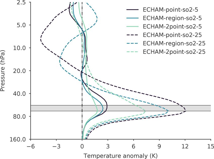
8622                               H. Franke et al.: Quasi-biennial oscillation response to stratospheric aerosol modification

Figure 3. Latitude–height cross section of the anomaly of the zonal mean residual vertical velocity w ∗ for the ECHAM simulations of
point-so2-25 (a), region-so2-25 (b), and 2point-so2-25 (c). Stippling indicates areas where anomalies are not significant at the 95 % level in
Student’s t test. Black contour lines show the anomaly of the zonal mean residual mass stream function χ in kilogram per second (kg s−1 ).
The thin solid contours indicate a clockwise circulation anomaly, and the dashed contours indicate a counterclockwise circulation anomaly.
The contour interval is logarithmic starting at 8 and −8 kg s−1 for the clockwise and counterclockwise anomalies, respectively, while the
0 kg s−1 contour is omitted. Yellow contour lines denote the residual vertical advection of zonal momentum −ω∗ uz with a contour interval
of 0.3 m s−1 d−1 , starting at 0.15 and −0.15 m s−1 d−1 . The solid lines indicate a positive anomaly, the dashed lines indicate a negative
anomaly, and the 0 m s−1 d−1 contour is omitted.

                                                                            However, despite the fact that QBO changes due to arti-
                                                                         ficial sulfur injections are frequently interpreted as a con-
                                                                         sequence of an increased residual tropical upwelling and a
                                                                         modification of thermal wind balance, one can not see both
                                                                         as two separate processes. In contrast, the acceleration of the
                                                                         BDC discussed in Sect. 3.1.2 is rather the mechanism by
                                                                         which thermal wind balance is re-established for the aerosol-
                                                                         induced lower-stratospheric temperature anomaly (Holton,
                                                                         2004). While the differences in the increase of w ∗ directly
                                                                         explain the different QBO responses to different injection
                                                                         strategies in a straightforward manner (see Sect. 3.1.2),
                                                                         in this section we show that the differences in the QBO
                                                                         response can be also linked directly to the meridional
                                                                         shape of the aerosol-induced lower-stratospheric temperature
                                                                         anomaly via thermal wind balance.
Figure 4. Latitude–height cross section of the zonal mean tempera-          As discussed in Sect. 3.1.1, an equatorial point injection
ture T in contr-000.                                                     results in a significant positive temperature anomaly cen-
                                                                         tered at the Equator (Fig. 2b). In the climatological mean –
                                                                         without artificial sulfur injections and represented by contr-
can set T y = 0 K km−1 at the Equator and apply the rule of              000 – the lower tropical stratosphere is much colder than
L’Hospital (Holton, 2004):                                               the lower midlatitudinal stratosphere (Fig. 4), leading to a
                                                                         poleward T y that is positive. The aerosol-induced warming
uz = −R(Hβ)−1 T yy .                                            (2)      abates the poleward T y (Fig. 5 a) within the lower tropical
                                                                         stratosphere between 40 and 80 hPa, which is accompanied
Within Eqs. (1) and (2), R denotes the gas constant for dry
                                                                         by a significant negative anomaly of T yy centered at the
air, H denotes the scale height, and β denotes the merid-
                                                                         Equator (Fig. 5b). Following Eq. (2), a negative anomaly of
ional gradient of the Coriolis parameter at the Equator. T yy
                                                                         T yy results in stronger westerly shear. Consequently, a strong
denotes the meridional curvature of the zonal mean tempera-
                                                                         westerly anomaly of the zonal mean zonal wind u is located
ture.

Atmos. Chem. Phys., 21, 8615–8635, 2021                                                     https://doi.org/10.5194/acp-21-8615-2021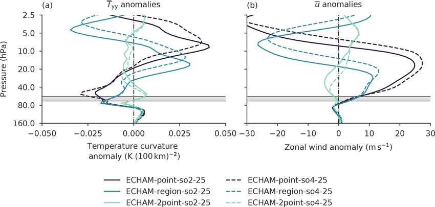
H. Franke et al.: Quasi-biennial oscillation response to stratospheric aerosol modification                                             8623

Figure 5. Latitude–height cross section of the anomaly of the meridional zonal mean temperature gradient T y (a, c, e) and of the anomaly of
the meridional zonal mean temperature curvature T yy (b, d, f) for the ECHAM simulations of point-so2-25 (a, b), region-so2-25 (c, d), and
2point-so2-25 (e, f). Stippling indicates areas where anomalies are not significant at the 95 % level in Student’s t test. Black contour lines
indicate the anomaly of the zonal mean zonal wind speed u in intervals of 3 m s−1 , with the thick black line denoting u = 0 m s−1 . Solid
lines denote a westerly anomaly; dashed lines denote an easterly anomaly.

on top of the injection layer in order to maintain thermal wind          fication close to the Equator is relatively small (Fig. 5c). Ac-
balance (Fig. 5b). This results in the observed constant west-           cordingly, also the negative anomaly of T yy and – following
erly QBO phase (Fig. 1b).                                                thermal wind balance (Eq. 2) – the induced anomaly of west-
   For region-so2-25, the QBO was also found to be locked                erly shear is weaker near the Equator compared to point-so2-
in a permanent westerly phase, but the vertical extent as well           25 (Fig. 5d). Consequently, the lower-stratospheric westerly
as the strength of the westerlies is weaker than for point-so2-          anomaly of u is weaker for region-so2-25 than for point-so2-
25, which is in agreement with the results of Niemeier and               25.
Schmidt (2017). The reason for the weaker westerlies is the                 For 2point-so2-25, the QBO was not found to be modified
meridionally more uniform temperature anomaly within the                 significantly, and it basically preserved its natural periodic-
lower tropical stratosphere (Fig. 2d). Therefore, the strongest          ity (Fig. 1k). Due to the extratropical injection locations, the
modifications of T y in the lower stratosphere are located               highest sulfate concentrations are located at approximately
poleward of approximately 20◦ N and 20◦ S, while its modi-               20◦ N and 20◦ S and so is the associated heating (Fig. 2e).

https://doi.org/10.5194/acp-21-8615-2021                                                    Atmos. Chem. Phys., 21, 8615–8635, 2021
8624 H. Franke et al.: Quasi-biennial oscillation response to stratospheric aerosol modification
(Fig. 1d, k). This comparison shows that within
uz ∼ R(Hβ)−1 L−2 T , (3)
which is often used as an approximation of thermal wind bal-
ance for QBO variations centered at the Equator (Baldwin
et al., 2001); the scaling factor L depends on the injection
strategy. Therefore, Eq. (3) cannot be used when comparing
the QBO response to different injection strategies.
Since it is the degree of tropical confinement of the arti-
ficial sulfate aerosols that is ultimately decisive for the ob-
served QBO response also when explaining the observed
QBO changes solely as the consequence of an increased
residual tropical upwelling, we will use thermal wind balance
in our argumentation throughout this study as it directly links
the observed QBO changes to the observed aerosol-induced
Figure 6. Vertical profile of the 5◦ N to 5◦ S mean temperature temperature anomalies.
anomaly for the 5 and 25 Tg(S) yr−1 injections simulated with
ECHAM. The horizontal grey bar marks the injection layer. The 3.2 Impact of injection rate
vertical dashed–dotted line marks a temperature anomaly of 0 K.
For the point and the region injection strategies, the QBO was
found to be impacted much less in our experiments with an
injection rate of 5 Tg(S) yr−1 than in those with an injection
Therefore, the lower-stratospheric temperature anomaly is rate of 25 Tg(S) yr−1 , and it basically maintained its oscil-
meridionally nearly uniform between approximately 15◦ N lating behavior (Fig. 1d, g). This is explained by the clearly
and 15◦ S (Fig. 2 f). Consequently, T y and T yy are only very lower tropical sulfate burden, which results from the lower
weakly modified between 40 and 80 hPa and between ap- injection rate. The sulfate burden determines the strength of
proximately 15◦ S and 15◦ N (Fig. 5e, f), and these anomalies the lower-stratospheric heating by absorption of OTLR and
are hardly statistically significant. Following thermal wind NIRR. Accordingly, the tropical mean temperature anoma-
balance, this implies that zonal wind anomalies in the lower lies are clearly weaker in our experiments with an injec-
stratosphere are small as well (Fig. 5e, f), which is in ac- tion rate of 5 Tg(S) yr−1 than in those ones with an injec-
cordance with the QBO in principle remaining in its natural tion rate of 25 Tg(S) yr−1 (Fig. 6). In contrast, the tempera-
shape. ture anomaly in the extratropical stratosphere is rather inde-
As discussed in Sect. 3.1.1, the negative temperature pendent of the injection rate for all injection strategies (not
anomalies above approximately 20 hPa have been induced shown), since absorptive heating is generally weak in this
dynamically due to an increased tropical upwelling and neg- region due to low values of OTLR and NIRR. Therefore,
ative temperature advection (see Aquila et al., 2014). While T y changes much less for a lower injection rate. The trop-
the corresponding anomalies of T y and T yy above 20 hPa ical mean anomalies of T yy in and slightly above the injec-
are of course still in thermal wind balance with the upper- tion layer are clearly smaller and vertically less extended for
stratospheric wind field (Fig. 5), it is important to mention an injection rate of 5 Tg(S) yr−1 compared to 25 Tg(S) yr−1
that this agreement does not imply causality in the way that (Fig. 7a). Following Eq. (2), this results in significantly
these upper-stratospheric temperature anomalies have caused smaller anomalies of the tropical mean zonal wind within
the lower-stratospheric westerly anomaly and QBO modifi- the lower stratosphere (Fig. 7b). For the point and the region
cation. injection strategies, the strength of the westerly anomaly is
Our results clearly show that differences in the QBO re- reduced by a factor of ∼ 10 when reducing the injection rate
sponse with respect to our three tested injection strategies from 25 to 5 Tg(S) yr−1 , and consequently the QBO is not
are linked to differences in the meridional structure of the locked in a permanent westerly phase (Fig. 1d, g). For the
aerosol-induced temperature anomaly. Therefore, the abso- 2point injection strategy, the tropical mean anomaly of T yy
lute strength of the aerosol-induced lower-stratospheric tem- is small for both tested injection rates (Fig. 7a). Accordingly,
perature anomaly does not permit a statement about the the QBO was found to be not modified significantly for ei-
strength of the QBO modification when comparing different ther tested injection rates when applying the 2point injection
injection strategies. For instance, the tropical (i.e., 5◦ N to strategy.
5◦ S) mean temperature anomaly within the injection layer is
more than twice as high in 2point-so2-25 than in point-so2-5
(Fig. 6). However, the QBO is heavily perturbed in point-
so2-5, while for 2point-so2-25 it remains nearly unchanged
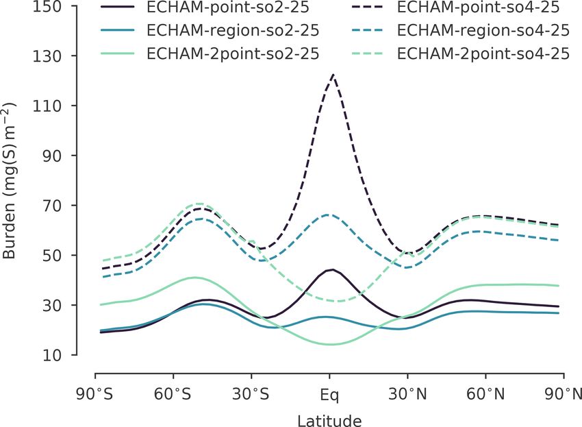
Atmos. Chem. Phys., 21, 8615–8635, 2021 https://doi.org/10.5194/acp-21-8615-2021H. Franke et al.: Quasi-biennial oscillation response to stratospheric aerosol modification 8625 Figure 7. Vertical profile of the 5◦ N to 5◦ S mean anomaly of the temperature curvature T yy (a) and the tropical mean anomaly of the zonal wind u (b) for the ECHAM simulations of a SO2 injection with an injection rate of 5 Tg(S) yr−1 (dashed) and 25 Tg(S) yr−1 (solid). The horizontal grey bar marks the injection layer. The vertical dashed–dotted line marks an anomaly of 0 K (100 km)−2 (a) and 0 m s−1 (b). 3.3 Impact of injection species For all three tested injection strategies, the response of the QBO is in principle independent of the injection species – SO2 or AM−SO4 – in our experiments with an injec- tion rate of 25 Tg(S) yr−1 (Fig. 1). This is reasonable, since the meridional distribution of the artificial sulfate aerosols, which can be seen as a proxy for the strength of the lower- stratospheric temperature anomaly, does in principle exhibit the same shape for both tested injection species except for different absolute values (Fig. 8). We showed that the modi- fication of the QBO depends clearly on the meridional struc- ture of the stratospheric temperature anomaly and is rather independent of its absolute value (Sect. 3.1.3). However, for the point and region injection strategies, the modification of the QBO was found to be slightly stronger Figure 8. Zonal mean artificial sulfate burden for the ECHAM sim- with respect to the strength and the vertical extent of the ulations of the SO2 injections (dashed lines) and the H2 SO4 in- lower-stratospheric westerlies when injecting AM−SO4 in- jections (solid lines) with an injection rate of 25 Tg(S) yr−1 as a stead of SO2 based on our experiments with an injection function of latitude. rate of 25 Tg(S) yr−1 (Fig. 1). This is a consequence of the in general higher sulfate burden, which results from an in- jection of AM−SO4 compared to an injection of SO2 . As jections. For the 2point injections of 25 Tg(S) yr−1 , an injec- described in Sect. 3.2, the accompanied stronger warming tion of AM−SO4 instead of SO2 causes the opposite effect as of the lower tropical stratosphere relative to the midlatitude it slightly weakens the positive anomaly of T yy and u within one results in a stronger modification of T yy (Fig. 9a). How- the tropics (Fig. 9). ever, the difference in the T yy anomaly between both injec- The reason for the higher sulfate burden obtained for an tion species is statistically significant at the 95 % level in injection of AM−SO4 compared to an injection of SO2 is Student’s t test only for the point injections. This causes a differences in microphysical processes. Due to weaker coag- stronger QBO westerly phase for an injection of AM−SO4 ulation and condensation, the sulfate particles stay on aver- compared to an injection of SO2 as indicated by the anoma- age smaller for an injection of AM−SO4 than for an injec- lies of u (Fig. 9b). The difference in the u anomaly between tion of SO2 for all tested injection scenarios (Fig. 10). This both injection species is statistically significant at the 95 % reduces their sedimentation and enhances their stratospheric level in Student’s t test for both the point and the region in- lifetime, which explains the larger sulfate burden. Addition- https://doi.org/10.5194/acp-21-8615-2021 Atmos. Chem. Phys., 21, 8615–8635, 2021
8626 H. Franke et al.: Quasi-biennial oscillation response to stratospheric aerosol modification
Figure 9. Vertical profile of the 5◦ N to 5◦ S mean anomaly of the temperature curvature T yy (a) and the tropical mean anomaly of the zonal
wind u (b) for the ECHAM simulations of injections with an injection rate of 25 Tg(S) yr−1 . The horizontal grey bar marks the injection
layer. The vertical dashed–dotted line marks an anomaly of 0 K (100 km)−2 (a) and 0 m s−1 (b).
Figure 10. Global mean aerosol size distributions focusing on AM−SO4 and coarse mode sulfate (CM−SO4 ) particles at 62 hPa, which
is the central level of the injection layer, for the ECHAM simulations of the point injections (a), the region injections (b), and the 2point
injections (c). The grey bar marks the size range in which the backscattering efficiency of an aerosol particle with a given wet radius is at
least 70 % (i.e., 0.12–0.40 µm) of its maximum value, which is achieved for aerosols with a wet radius of 0.30 µm and marked by a thick
solid black line (Dykema et al., 2016).
ally, smaller sulfate particles have a higher backscattering ef- 4 Comparison between ECHAM and CESM
ficiency (Fig. 10). Therefore, the RF efficiency (RF per in-
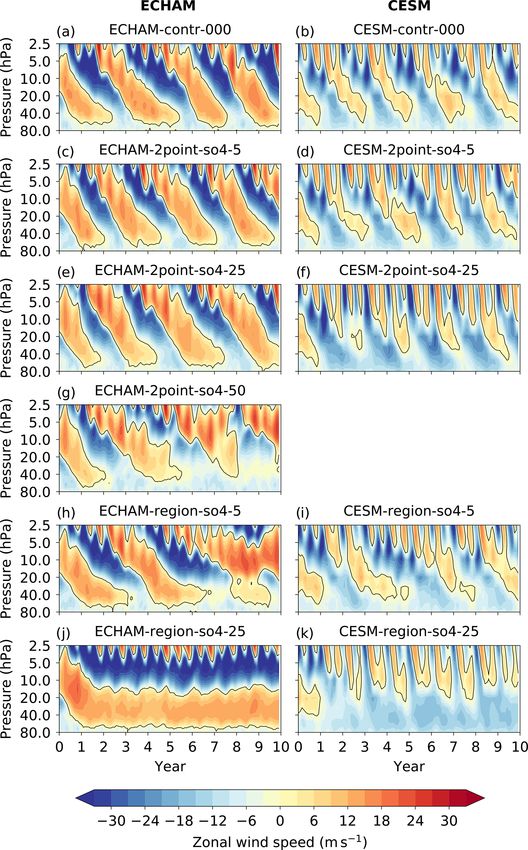
jected amount of sulfur) is also significantly higher for an Both models simulate a reasonable QBO in the control sim-
injection of AM−SO4 than for an injection of SO2 (Fig. 11). ulation (Fig. 12a, b). With roughly 32 months the simulated
The required injection rate to achieve a given RF is conse- QBO period of ECHAM is slightly longer than the one sim-
quently clearly smaller for an injection of AM−SO4 com- ulated in CESM, which is approximately 27 months. Both
pared to an injection of SO2 . For example, to counteract a compare well to the observed period of 28 months on average
RF of 4.0 W m−2 as proposed in the GeoMIP6 experiment (Naujokat, 1986). The simulated QBO winds, especially the
G6sulfur (Kravitz et al., 2015), an injection of SO2 would QBO westerlies, are substantially stronger in ECHAM than
require injection rates of more than 25 Tg(S) yr−1 , while an in CESM at altitudes above 40 hPa. Accordingly, the QBO
injection rate of about 10 to 12.5 Tg(S) yr−1 would be suffi- easterly phases are longer and relatively stronger in CESM
cient for an injection of AM−SO4 , depending on the injec- at altitudes below 30 hPa. These general differences of the
tion strategy (Fig. 11). The higher RF efficiency of an injec- simulated QBO have to be considered when comparing the
tion of H2 SO4 should therefore be considered when compar- QBO response to different SAM scenarios in both models.
ing the QBO response between both tested injection species. In the following two sections, the QBO response to the
2point and region injections will be compared for ECHAM
Atmos. Chem. Phys., 21, 8615–8635, 2021 https://doi.org/10.5194/acp-21-8615-2021H. Franke et al.: Quasi-biennial oscillation response to stratospheric aerosol modification 8627
Figure 11. Global mean top-of-atmosphere (TOA) all-sky net RF
exerted by artificial sulfate aerosols as a function of injection rate.
The dotted black line marks a RF of −4 W m−2 .
and CESM based on the injection of AM−SO4 only. For an
injection of SO2 instead of AM−SO4 , the observed charac-
teristics of the QBO remain basically the same in both mod-
els (See Sect. 3.3) and corresponding plots for an injection
of SO2 can be found in the Supplement. A comparison of
the QBO response to the point injection strategy is not possi-
ble, since the point injection is not part of the accumH2SO4
experimental protocol and was, therefore, not performed by
CESM.
4.1 2point injection strategy
For the 2point injections of AM−SO4 simulated in ECHAM,
the periodicity and strength of the QBO are basically not Figure 12. Time–height cross sections of the 5◦ N to 5◦ S mean
zonal wind in the stratosphere over the simulation period of 10 years
modified for the tested injection rates of 5 and 25 Tg(S) yr−1
for the AM−SO4 injection scenarios in ECHAM (left column) and
(Fig. 12c, e). However, for an injection rate of 25 Tg(S) yr−1 CESM (right column). The first row shows the control simulation,
a slight easterly anomaly of up to −3 m s−1 has been noticed the second row shows the 2point injections of 5 Tg(S) yr−1 , the
at approximately 40 hPa and 5◦ S (Fig. 13 c), which is at the third row shows the 2point injections of 25 Tg(S) yr−1 , the fifth
edge of extreme natural variability based on Student’s t test. row shows the region injections of 5 Tg(S) yr−1 , and the sixth row
In CESM, the QBO is also not modified much relative to shows the region injections of 25 Tg(S) yr−1 . The 2point injection
the control simulation for the 2point injections with an in- of 50 Tg(S) yr−1 was only performed with ECHAM and is shown
jection rate of 5 Tg(S) yr−1 (Fig. 12d). For an injection rate in the fourth row. The solid black line marks a tropical mean zonal
of 25 Tg(S) yr−1 , the QBO basically maintains its oscillat- wind speed of 0 m s−1 .
ing behavior in CESM as well (Fig. 12f) but with clearly
stronger easterlies and weaker westerlies at altitudes below
20 hPa compared to the control simulation. Hemisphere. The anomaly of T y also shows basically the
Nevertheless, the QBO responds qualitatively similar to same spatial structure in both models as the usually pos-
a 2point injection of AM−SO4 in both models, which is itive poleward T y between approximately 80 and 40 hPa
clearly shown by Fig. 12c–f. The spatial structure of the u strengthens statistically significantly. For a given injection
anomalies, indicated by the contour lines in Fig. 13, does rate, this strengthening – located approximately between 80
in general agree for both models and both tested injection and 40 hPa and between 20◦ S and 20◦ N – is clearly stronger
rates (Fig. 13a–d). For an injection rate of 25 Tg(S) yr−1 , and vertically more extended in CESM (Fig. 13c, d), which
it shows a lower-stratospheric easterly anomaly centered at explains the stronger easterly anomaly observed in CESM as
approximately 40 hPa and 5◦ S and an upper-stratospheric a consequence of thermal wind balance (Eq. 1).
westerly anomaly, which further extends into the Northern
https://doi.org/10.5194/acp-21-8615-2021 Atmos. Chem. Phys., 21, 8615–8635, 20218628 H. Franke et al.: Quasi-biennial oscillation response to stratospheric aerosol modification
Figure 14a demonstrates the reason for the more signifi-
cant strengthening of the poleward T y in CESM. In accor-
dance with Niemeier et al. (2020), the sulfate burden for
a given injection rate is substantially larger in CESM than
in ECHAM, which is predominantly due to a stronger w ∗ .
Given the characteristic meridional distribution of sulfate
particles for a 2point injection, this results in a higher sulfate
burden in the subtropical stratosphere relative to the tropical
one in CESM (Fig. 14a). This is the reason for the stronger
modification of T y for a given injection rate in CESM com-
pared to ECHAM.
Following Niemeier et al. (2020), we therefore performed
an ECHAM simulation of a 2point injection which results
in approximately the same global mean sulfate burden and
the same meridional distribution of sulfate particles like
the CESM simulation of a 2point injection with an injec-
tion rate of 25 Tg(S) yr−1 . This is the case for an injec-
tion of 50 Tg(S) yr−1 in ECHAM (Fig. 14a). As visible in
Figure 12g, the QBO easterly phases are substantially pro-
longed also in ECHAM for injections with an injection rate
of 50 Tg(S) yr−1 . In this simulation, the QBO westerlies in
the lower stratosphere at altitudes below 20 hPa are clearly
weaker than in the control simulation (Fig. 12g). Overall, the
spatiotemporal structure of the QBO jets agrees reasonably
well between the CESM simulation with an injection rate of
25 Tg(S) yr−1 and the ECHAM simulation of 50 Tg(S) yr−1 ,
given the general differences of the simulated QBO of both
models. Additionally, also the anomalies of T y and u agree
reasonably well with each other (Fig. 13d, e). This indicates
that the QBO does in principle respond similarly to a 2point
injection of AM−SO4 in both models but that this response
is more sensitive to an increase of the injection rate in CESM
than in ECHAM, which is in agreement with Niemeier et al.
(2020). Nevertheless, the QBO response is still stronger in
CESM than in ECHAM, and the reason for this has not been
conclusively determined.
4.2 Region injection strategy
Figure 13. Latitude–height cross sections of the anomaly of the In contrast to the 2point injections, the response of the
meridional zonal mean temperature gradient T y for the AM−SO4 QBO to a region injection of AM−SO4 is fundamen-
injection scenarios in ECHAM (left column) and in CESM (right tally different in ECHAM and CESM. For an injection
column). Stippling indicates areas where anomalies are not signifi- rate of 5 Tg(S) yr−1 , the QBO slows down in both models
cant at the 95 % level in Student’s t test. Black contour lines indicate with lower-stratospheric winds being predominantly west-
the anomaly of the zonal mean zonal wind speed u in intervals of erly in ECHAM, while being more easterly in CESM
3 m s−1 , with the thick black line denoting u = 0 m s−1 . Solid lines (Fig. 12h, i). For an injection rate of 25 Tg(S) yr−1 , the lower-
denote a westerly anomaly, while dashed lines denote an easterly stratospheric QBO is locked in a permanent westerly phase in
anomaly. The first row shows the 2point injections of 5 Tg(S) yr−1 ,
ECHAM, while it is locked in a permanent easterly phase in
the second row shows the 2point injections of 25 Tg(S) yr−1 , the
fourth row shows the region injections of 5 Tg(S) yr−1 , and the fifth
CESM (Fig. 12j, k). Accordingly, in ECHAM u has a west-
row shows the region injections of 25 Tg(S) yr−1 . The 2point in- erly anomaly of up to +12 m s−1 at the Equator at a pressure
jection of 50 Tg(S) yr−1 was only performed with ECHAM and is level of approximately 25 hPa, while in CESM it has an east-
shown in the third row. erly anomaly of more than −10 m s−1 at the same location
(Fig. 13h, i).
For ECHAM, the results are explained by the weaken-
ing of the usually positive poleward T y due to the aerosol-
Atmos. Chem. Phys., 21, 8615–8635, 2021 https://doi.org/10.5194/acp-21-8615-2021You can also read