Distributed summer air temperatures across mountain glaciers in the south-east Tibetan Plateau: temperature sensitivity and comparison with ...
←
→
Page content transcription
If your browser does not render page correctly, please read the page content below
The Cryosphere, 15, 595–614, 2021
https://doi.org/10.5194/tc-15-595-2021
© Author(s) 2021. This work is distributed under
the Creative Commons Attribution 4.0 License.

Distributed summer air temperatures across mountain glaciers in
the south-east Tibetan Plateau: temperature sensitivity and
comparison with existing glacier datasets
Thomas E. Shaw1 , Wei Yang2,3 , Álvaro Ayala4 , Claudio Bravo5 , Chuanxi Zhao2 , and Francesca Pellicciotti1,6
1 Federal Institute for Forest, Snow and Landscape Research (WSL), Birmensdorf, Switzerland
2 Key Laboratory of Tibetan Environment Changes and Land Surface Processes, Institute of Tibetan Plateau Research,
Chinese Academy of Sciences (CAS), Beijing, China
3 CAS Center for Excellence in Tibetan Plateau Earth Sciences, Beijing 100101, China
4 Centre for Advanced Studies in Arid Zones (CEAZA), La Serena, Chile
5 School of Geography, University of Leeds, Leeds, UK
6 Department of Geography, Northumbria University, Newcastle, UK

Correspondence: Thomas E. Shaw (thomas.shaw@wsl.ch)

Received: 15 July 2020 – Discussion started: 12 August 2020
Revised: 17 December 2020 – Accepted: 30 December 2020 – Published: 9 February 2021

Abstract. Near-surface air temperature (Ta ) is highly im-          ary layer flow, warm up-valley winds or debris/valley heat-
portant for modelling glacier ablation, though its spatio-          ing effects) which are evident only beyond ∼ 70 % of the
temporal variability over melting glaciers still remains            total glacier flowline distance. Our results therefore suggest
largely unknown. We present a new dataset of distributed            a strong role of local effects in modulating temperature sen-
Ta for three glaciers of different size in the south-east Ti-       sitivity close to the glacier terminus, although further work
betan Plateau during two monsoon-dominated summer sea-              is still required to explain the variability of these effects for
sons. We compare on-glacier Ta to ambient Ta extrapolated           different glaciers.
from several local off-glacier stations. We parameterise the
along-flowline sensitivity of Ta on these glaciers to changes
in off-glacier temperatures (referred to as “temperature sensi-
tivity”) and present the results in the context of available dis-   1   Introduction
tributed on-glacier datasets around the world. Temperature
sensitivity decreases rapidly up to 2000–3000 m along the           Near-surface air temperature (Ta ) is one of the dominant con-
down-glacier flowline distance. Beyond this distance, both          trols on glacier energy and mass balance during the ablation
the Ta on the Tibetan glaciers and global glacier datasets          season (Petersen et al., 2013; Gabbi et al., 2014; Sauter and
show little additional cooling relative to the off-glacier tem-     Galos, 2016; Maurer et al., 2019; Wang et al., 2019), though
perature. In general, Ta on small glaciers (with flowline dis-      modelling its spatio-temporal behaviour above melting ice
tances < 1000 m) is highly sensitive to temperature changes         surfaces remains a challenge. The absence of distributed
outside the glacier boundary layer. The climatology of a            information regarding Ta has favoured the use of simple,
given region can influence the general magnitude of this            space–time invariant relationships of Ta with elevation, typ-
temperature sensitivity, though no strong relationships are         ically that of the free-air environmental lapse rate (ELR). A
found between along-flowline temperature sensitivity and            free-air ELR cannot be reliably used to estimate near-surface
mean summer temperatures or precipitation. The terminus of          air temperatures above melting glaciers, where steep gradi-
some glaciers is affected by other warm-air processes that          ents are found within 10 m of the surface under warm ambi-
increase temperature sensitivity (such as divergent bound-          ent (off-glacier) conditions (van den Broeke, 1997; Greuell
                                                                    and Böhm, 1998; Oerlemans, 2001; Oerlemans and Griso-

Published by Copernicus Publications on behalf of the European Geosciences Union.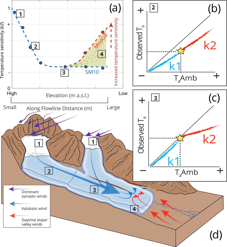
596                                                       T. E. Shaw et al.: Distributed air temperature on mountain glaciers

gono, 2002; Ayala et al., 2015). As a result, any extrapolation      ing flowline distances due to sensible heat exchange and adi-
of Ta observations from an off-glacier location, particularly        abatic heating (Greuell and Böhm, 1998). It adds a warming
those at lower elevations, are likely to lead to an overestima-      factor based upon on-glacier observations in the lower sec-
tion of snow and ice ablation in energy balance and enhanced         tions of the glacier (e.g. at the greatest flowline distances) to
temperature index melt simulations (e.g. Petersen and Pel-           account for additional processes of adiabatic warming (Ay-
licciotti, 2011; Pellicciotti et al., 2014; Shaw et al., 2017).      ala et al., 2015) (Fig. 1a). The ModGB approach has been
While models applying the degree day approach can make               successively applied at other glacier sites around the world
use of off-glacier temperatures as forcing because they are          (Shaw et al., 2017; Troxler et al., 2020), though the question
heavily reliant on calibration, for energy balance models and        of its transferability remains open (Troxler et al., 2020).
models of intermediate complexity (Pellicciotti et al., 2005;           In this way, the ModGB method operates on the physical
Ragettli et al., 2016) it is key to resolve the air temperature      principles of the glacier boundary layer (Greuell and Böhm,
distribution over glaciers, especially for turbulent flux calcu-     1998), though it corrects for relative warming on the lower
lations and typical parameterisations of incoming longwave           portion of glacier (Ayala et al., 2015). To establish the mag-
radiation.                                                           nitude of this warming, however, along-flowline data in the
    This problem has been long understood (Greuell et al.,           lower portion of the glacier are essential. Because the avail-
1997; Greuell and Böhm, 1998), but only within the last              able distribution of on-glacier observations is often limited
decade have studies approached it in more detail (Petersen           and rarely extends for the entire length of the glacier flow-
et al., 2013; Ayala et al., 2015; Carturan et al., 2015; Shaw        line, this additional correction for warming associated with
et al., 2017; Bravo et al., 2019a; Troxler et al., 2020). Un-        the unknown parameters of ModGB can lead to high variabil-
til recently, modelling studies have relied upon simple lapse        ity in Ta estimates on the lower glacier ablation zone (Trox-
rates (including the ELR) and/or single bias offset values           ler et al., 2020) (Fig. 1a). In contrast to this, the statistical
to account for the cooling effect of the near-surface air on         method of Shea and Moore (2010) provides a more simpli-
glacier (Arnold et al., 2006; Nolin et al., 2010; Ragettli et al.,   fied estimation that has fewer assumptions and parameters,
2016). The variations of Ta along the glacier flowline (de-          though it does not explicitly account for physical processes
fined following Shea and Moore, 2010, as the horizontal dis-         thought to be the cause of relative warming on the glacier ter-
tance from an upslope summit or ridge), however, are much            minus. It also provides a parameter that more explicitly rep-
more complex (Ayala et al., 2015; Shaw et al., 2017), though         resents the glacier temperature sensitivity of the on-glacier Ta
a lack of available data usually restricts one’s ability to ap-      (defined here as the ratio of changes in observed Ta on glacier
propriately model this variable.                                     to changes in Ta Amb – Fig. 1b and c). Despite its more con-
    To date, two main, simplified model approaches have              ceptual nature, because of its ease of applicability, typical of
been developed and tested to represent air temperature over          a more simplistic statistical approach, we adopt the Shea and
glaciers (Fig. 1a). The first is the statistical model by Shea       Moore (2010) method to further investigate along-flowline
and Moore (2010) developed to reconstruct Ta across glaciers         Ta in this study.
of varying size in western Canada from ambient temperature              To date, few studies have investigated the variability of
records. This approach considered the ratios of observed on-         distributed, on-glacier Ta at different sites around the world.
glacier temperature and estimated ambient temperature for            As such, the transferability of temperature estimation models
the elevation of a given point on a glacier (hereafter Ta Amb).      and/or model parameters remains mostly unknown, and anal-
The authors calculated two ratios from a piecewise regres-           ysis of individual glacier sites, while beneficial to process un-
sion above and below a critical threshold temperature for the        derstanding, may not advance the science on how to treat the
onset of the glacier katabatic boundary layer (KBL – see             on-glacier Ta in models. In this study, we use new datasets
Sect. 4.3). The parameterisations that operate as a function         of on-glacier temperature observations on three glaciers of
of the along-flowline distance have since been tested by Car-        varying size in the south-east Tibetan Plateau. We analyse
turan et al. (2015) and Shaw et al. (2017) on smaller glaciers       the main controls on along-flowline Ta and its temperature
in different parts of the Italian Alps. Carturan et al. (2015)       sensitivity and present these new findings in the context of
found that the original published parameterisations were suf-        11 other on-glacier observations around the world.
ficient to explain Ta on small, fragmenting glaciers up to              Specifically we aim to (i) understand the variability of
flowline distances of ∼ 2000 m. However, investigation by            Ta with the along-flowline distances at three glaciers in the
Shaw et al. (2017) on a small alpine glacier found a pattern         south-east Tibetan Plateau, (ii) identify and quantify the tem-
of along-flowline Ta that was better described by an alter-          perature sensitivity of on-glacier Ta for different meteorolog-
native, thermodynamic model approach. This second, physi-            ical conditions and glacier sizes, and (iii) parameterise the
cally oriented approach was developed by Ayala et al. (2015)         along-flowline Ta using the Shea and Moore (2010) method
to account for a relative warming effect evident on the ter-         for the Tibetan glaciers and discuss it in the context of glob-
mini of some mountain glaciers when compared to upper el-            ally derived, published datasets of on-glacier air tempera-
evations. The modified model (termed “ModGB” in the liter-           tures.
ature) accounts for the down-glacier cooling of Ta at increas-

The Cryosphere, 15, 595–614, 2021                                                         https://doi.org/10.5194/tc-15-595-2021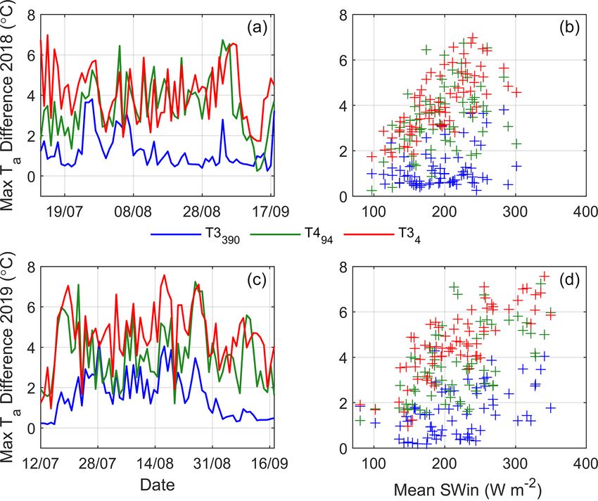
T. E. Shaw et al.: Distributed air temperature on mountain glaciers                                                                         597

Figure 1. A schematic diagram to describe the temperature sensitivity of on-glacier air temperature (Ta ) to the extrapolated ambient temper-
ature (Ta Amb) at given elevations/flowline distances on a mountain glacier. Points 1–4 indicate locations of interest that are linked between
panels. Panel (a) indicates the along-flowline k2 temperature sensitivities to Ta Amb, considering the differences represented by the models of
SM10 and ModGB for glacier termini (see text). Panels (b) and (c) represent the differences of k1 (blue) and k2 (red) sensitivities observed
in the data at different theoretical locations on the glacier, the latter of which shows the theoretical parameterisation presented by Shea and
Moore (2010). The yellow stars indicate the calculated threshold for katabatic onset (T ∗ in the text). Panel (d) represents an idealised case of
katabatic and valley/synoptic wind interactions that potentially dictate the along-flowline structure of on-glacier temperature sensitivity and
thus Ta estimation.

2   Study site                                                             smaller valley glaciers (2.51 and 0.37 km2 , respectively) that
                                                                           have termini at higher elevations (elevation ranges of 5000–
The study glaciers are located in the upper Parlung Zangbo                 5635 and 5195–5469 m a.s.l., respectively). The glaciers of
(also know as the Parlung Tsangpo) river catchment in the                  the catchment were classified by Yang et al. (2013) as hav-
south-east Tibetan Plateau (29.24◦ N, 96.93◦ E – Fig. 2), a                ing a spring-accumulation regime and the longest rain sea-
region characterised by a summer monsoon climate that typi-                son of the entire Tibetan Plateau. The upper Parlung Zangbo
cally intrudes via the Brahmaputra Valley (Yang et al., 2011).             river catchment has a mean summer (1979–2019) annual air
We present data for three maritime-type valley glaciers in the             temperature of ∼ 2 ◦ C (at 4600 m a.s.l.), and temperatures in
Parlung Zangbo catchment: Parlung Glacier Number 4 (here-                  the wider region have been shown to be increasing since the
after Parlung4), Parlung Glacier Number 94 (Parlung94)                     mid-1990s (Yang et al., 2013). The glaciers of this region
and Parlung Glacier Number 390 (Parlung390). Parlung4                      have been shown to be very sensitive to temperature changes,
(Fig. 2d) is ∼ 10.8 km2 , is north-north-east facing and has               though with a lower sensitivity of mass balance to elevation
an elevation range of 4659–5939 m a.s.l. (Ding et al., 2017).              compared to other continental glaciers of the Tibetan Plateau
Glaciers Parlung94 (Fig. 2c) and Parlung390 (Fig. 2e) are

https://doi.org/10.5194/tc-15-595-2021                                                                The Cryosphere, 15, 595–614, 2021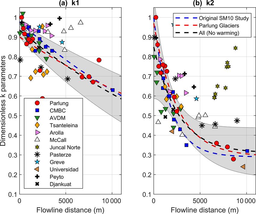
598                                                      T. E. Shaw et al.: Distributed air temperature on mountain glaciers

(Wang et al., 2019). Because Tibetan glaciers are shrinking        1997; Oerlemans and Grisogono, 2002), 95 % of hourly dif-
and fragmenting, the accurate estimation of on-glacier tem-        ferences were < 1 ◦ C (Fig. S1 in the Supplement). For on-
peratures is relevant for investigating and modelling their        glacier stations at large flowline distances (Fig. 2), large dif-
temperature sensitivity (Carturan et al., 2015). However, to       ferences are considered less likely given the good ventila-
date, no studies regarding the distribution of on-glacier tem-     tion provided to the sensors within the KBL. While obser-
perature have been performed within the Tibetan Plateau.           vations at short flowline distances with calm conditions and
                                                                   high incoming radiation may result in larger differences up
                                                                   to ∼ 1 ◦ C (Troxler et al., 2020), we apply a ±0.5 ◦ C uncer-
3     Data                                                         tainty for analysis of distributed Ta . For the instantaneous dif-
                                                                   ferences > 1 ◦ C, wind speeds at AWS_On were < 2 m s−1 .
3.1    Meteorological observations
                                                                   Wind speeds for P90 conditions were otherwise in excess of
We present the observations of Ta from a total of 20 air tem-      3–4 m s−1 , though no other observations of on-glacier wind
perature logger locations (Table 1), 13 of which are situated      speed are available at higher elevations. We note that in the
on glacier (4680–5369 m a.s.l.) and seven off glacier (4648–       absence of an artificially ventilated Ta measurement as a ref-
5168 m a.s.l.). These stations (hereafter referred to as “T log-   erence (e.g. Georges and Kaser, 2002; Carturan et al., 2015),
gers”) observed Ta at a 2 m height using HOBO U23-001              a true uncertainty value cannot be prescribed for the Ta obser-
temperature–relative-humidity sensors (accuracy +0.21 ◦ C)         vations of our study and only assumed based upon previous
within double-louvred, naturally ventilated radiation shields      literature. This is discussed further in Sect. 6.
(HOBO RS1) mounted on free-standing tripods. The T log-
                                                                   3.3    Elevation information
gers recorded data in 10 min intervals that are averaged to
hourly data for analysis. We identify a common observation         We use the 12.5 m Alos Palsar (ASF DAAC, 2020) digi-
period over the summers of 2018 and 2019 that ranges from          tal elevation model (DEM) to obtain elevation information
12 July–18 September. For these date ranges, we observe            for the catchment (Fig. 2b). Flowline distances (m) for each
only small data gaps for some T loggers (< 1 % of the to-          glacier are calculated from the TopoToolbox functions in
tal period). We apply the nomenclature of T XG , whereby X         MATLAB (Schwanghart and Kuhn, 2010), following Trox-
refers to the T -logger number on each glacier and G refers        ler et al. (2020). We note that the methodology for flowline
to the glacier number (Table 1).                                   generation is not currently uniform among all studies of this
   We additionally present Ta observations at two auto-            type (Shea and Moore, 2010; Ayala et al., 2015; Carturan
matic weather stations (AWS) at elevations ∼ 4600 m a.s.l.         et al., 2015; Shaw et al., 2017; Bravo et al., 2019a; Troxler
(off glacier, henceforth AWS_Off) and ∼ 4800 m a.s.l. (on          et al., 2020) and may produce some differences in the cal-
Parlung4, henceforth AWS_On) for the same time pe-                 culated distances close to the lateral borders of the glaciers.
riod (Fig. 2). The AWS Ta observations are provided by             In addition, the generated flowlines may also be dependent
Vaisala HMP60 temperature–relative-humidity sensors (ac-           upon the quality and resolution of the DEM available. How-
curacy +0.5 ◦ C) housed in naturally ventilated, Campbell          ever, we do not analyse lateral Ta variations in this study and
41005-5 radiation shields. We obtain information regard-           consider the impact of varying methods for flowline gener-
ing incoming shortwave radiation and relative humidity             ation to be negligible when assessing observations at a few
(AWS_Off), on-glacier wind speed (AWS_On), and free-air            selected points on the glacier.
wind speed and direction (ERA5 – C3S, 2017). We use these
data to explore the relationships of hourly on- and off-glacier
temperatures (Sect. 4.2) for different prevailing conditions.      4     Methods

3.2    Intercomparison of air temperature observations             Our methods consist of (1) aggregating temperature obser-
                                                                   vations based on off-glacier temperatures and prevailing me-
To evaluate the comparability of air temperature measure-          teorological conditions, (2) generating off-glacier tempera-
ments, we calculate the hourly divergence of two naturally         ture lapse rates to compare on- and off-glacier temperatures
ventilated Ta observations for the whole period between T 44       at the same elevation, and (3) estimating the near-surface
and AWS_On (Fig. 2d), which are located within a few me-           temperature sensitivity by fitting parameters to the model of
tres of horizontal distance of each other on Parlung4 Glacier.     Shea and Moore (2010). The following subsections outline
A test of absolute differences between the two stations re-        the subgrouping (Sect. 4.1) and off-glacier Ta distribution
sulted in a mean of < 0.4 ◦ C for all hours (n = 3312) and         (Sect. 4.2) methodologies. The model parameterisations of
∼ 0.5 ◦ C for the warmest 10 % of the hours of ambient tem-        Shea and Moore (2010) and application to Tibetan and global
perature at AWS_Off. We find that for these warm hours             datasets are described in Sect. 4.3 and 4.4, respectively.
(hereafter referred to as “P90” – Ayala et al., 2015; Shaw
et al., 2017; Troxler et al., 2020), when the KBL develop-
ment is theoretically at its strongest (e.g. van den Broeke,

The Cryosphere, 15, 595–614, 2021                                                       https://doi.org/10.5194/tc-15-595-2021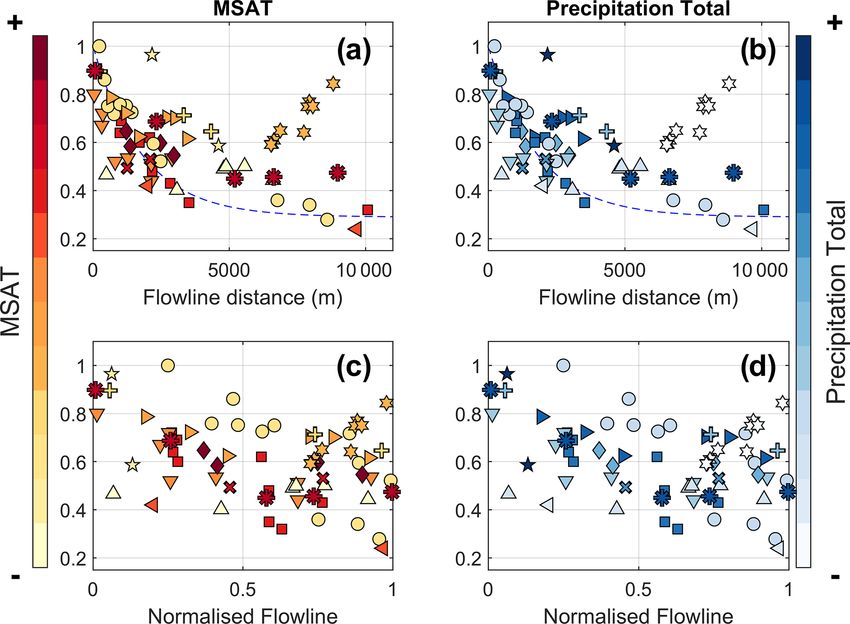
T. E. Shaw et al.: Distributed air temperature on mountain glaciers                                                                       599

Figure 2. The location of Parlung catchment in Tibet (a) and a map of the Parlung glaciers (b) with the study glaciers, Parlung94 (c), Parlung4
(d) and Parlung390 (e). Off-glacier and on-glacier AWS and T -logger locations are shown (without glacier number suffix – see Table 1).
Panel (b) shows the elevation of the catchment (DEM source: Alos Palsar), and Panels (c)–(e) show the calculated flowline distances based
upon TopoToolbox (scales vary).

4.1   Subgrouping on-glacier air temperature                              evaluate how strong the linear relationship of on-glacier Ta
      observations                                                        with elevation and flowline distance is for these subgroups
                                                                          using the coefficient of determination (R 2 ). For a compari-
Subgrouping allows one to interpret general causal factors                son to previous studies (Petersen and Pellicciotti, 2011; Shaw
that dictate on-glacier behaviour. We subgroup our on-glacier             et al., 2017), we also report the equivalent on-glacier lapse
observations by 10th and 90th percentiles (P10 = the coldest              rate that would be calculated for the above conditions.
10 %, P90 = the warmest 10 %) of off-glacier Ta at AWS_Off
(Fig. 2a). Following the methodology of previous studies                  4.2   Comparison of on- and off-glacier air temperature
(Ayala et al., 2015; Shaw et al., 2017; Troxler et al., 2020),
we bin all contemporaneous observations of on-glacier Ta at               We extrapolate AWS_Off Ta records to the elevation of each
each T logger that correspond to the same hours as the cold-              on-glacier T logger (Table 1) to quantify the differences be-
est (P10) and warmest (P90) observations at AWS_Off. We                   tween ambient and on-glacier Ta (Fig. 1a). We derive an

https://doi.org/10.5194/tc-15-595-2021                                                              The Cryosphere, 15, 595–614, 2021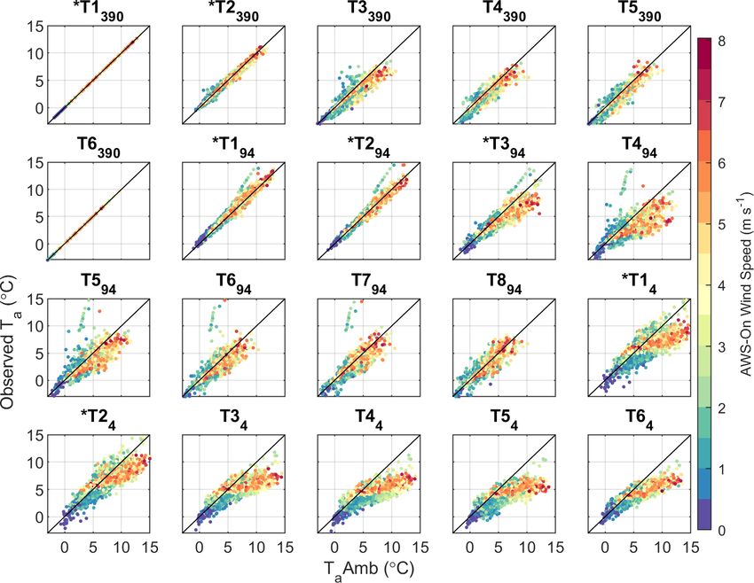
600                                                          T. E. Shaw et al.: Distributed air temperature on mountain glaciers

Table 1. Details of each AWS/T -logger station used in this analysis including the calculated flowline distances.

                        Station      Latitude    Longitude     Elevation (m a.s.l.)   Flowline (m)    On/off glacier
                        AWS_Off        29.314       96.955                   4588                –    off
                        AWS_On         29.500       97.009                   4808                –    off
                        T 1390         29.348       97.022                   5095                –    off
                        T 2390         29.352       97.020                   5168                –    off
                        T 3390         29.354      97.0202                   5258              770    on
                        T 4390         29.356       97.020                   5310              544    on
                        T 5390         29.357       97.019                   5335              420    on
                        T 6390         29.359       97.018                   5377              224    on
                        T 194          29.621       97.218                   4965                –    off
                        T 294          29.417        96.99                   4992                –    off
                        T 394          29.635       96.975                   5086                –    off
                        T 494          29.596       97.065                   5138             2481    on
                        T 594           29.56       97.067                   5174             2215    on
                        T 694          29.466       97.023                   5302             1411    on
                        T 794          29.434       97.080                   5280             1208    on
                        T 894          29.399       97.097                   5331              988    on
                        T 14           29.271       96.968                   4690                –    off
                        T 24           29.368       96.935                   4769                –    off
                        T 34           29.298       97.168                   4806             8589    on
                        T 44           29.298       97.168                   4809             7940    on
                        T 54           29.496       97.126                   4841             7505    on
                        T 64           29.403       97.068                   4909             6765    on

hourly variable lapse rate between AWS_Off and off-glacier               tions of the along-flowline distance (DF):
T loggers T 194 , T 294 and T 1390 to construct a catchment
lapse rate where the origin of the calculated regression must            k1 = β1 exp(β2 DF),                                          (2)
pass through the elevation of AWS_Off (see Supplement,                   k2 = β3 + β4 exp(β5 DF),                                     (3)
Fig. S2). These T loggers are assumed to be unaffected by
the glacier boundary layer, and we consider this the best                where βi represents the fitted coefficients. Following the sug-
available approach to estimate the ambient lapse rate for the            gestion of Carturan et al. (2015), we implement a relation
catchment. We compare the hourly estimates of the extrap-                against the flowline that estimates the threshold temperature
olated off-glacier Ta (Ta Amb) with the observations at each             for onset of katabatic effects (T ∗ ) at a given distance as
on-glacier T logger in order to (i) quantify the differences
and how they relate to meteorological conditions and glacier                      C1DF
                                                                         T∗ =            ,                                            (4)
flowline distance and (ii) parameterise the along-flowline                       C2 + DF
temperature sensitivity to Ta Amb following Shea and Moore               where C1 (6.61) and C2 (436.04) are the fitted coefficients
(2010) (Sect. 4.3).                                                      of Carturan et al. (2015). We calculate k1 and k2 at each T -
                                                                         logger station using the linear regression of observed Ta and
4.3    Estimation of on-glacier temperature sensitivity                  Ta Amb above and below T ∗ (Fig. 1) as derived from Eq. (4).
                                                                         We note that the parameter k2 holds a greater significance for
The Shea and Moore (2010) approach (hereafter “SM10”)                    modelling Ta (Fig. 1a), as this more closely represents the
estimates on-glacier Ta using Ta Amb at a given elevation by             “climatic sensitivity” reported by previous works (Greuell
                                                                         et al., 1997; Greuell and Böhm, 1998; Oerlemans, 2001;
           T 1 + k2(Ta Amb − T ∗ ), Ta Amb ≥ T ∗ ,

Ta =                                                            (1)      2010), whereas k1 represents the ratio of above-glacier and
           T 1 − k1(T ∗ − Ta Amb), Ta Amb < T ∗ ,                        free-air temperatures without a katabatic effect that has been
                                                                         shown to relate more closely to Ta Amb (Shea and Moore,
where T ∗ (◦ C) represents the threshold ambient temperature             2010; Shaw et al., 2017). For this study, we therefore pay par-
for the onset of katabatic flow and T 1 is the corresponding             ticular attention to the k2 sensitivities on the Parlung glaciers
threshold Ta on the glacier. Parameters k1 and k2 are the tem-           and assess their relationship to along-flowline distance.
perature sensitivities (ratio of on-glacier Ta to Ta Amb) below
and above the threshold T ∗ (Fig. 1b and c). k1 and k2 were
parameterised in the original study using exponential func-

The Cryosphere, 15, 595–614, 2021                                                               https://doi.org/10.5194/tc-15-595-2021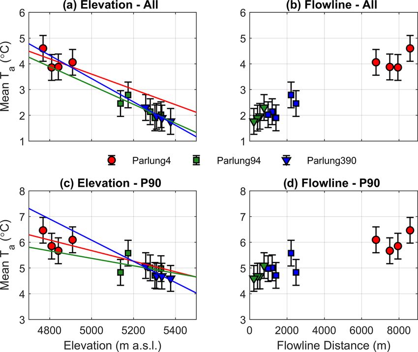
T. E. Shaw et al.: Distributed air temperature on mountain glaciers                                                             601

4.4    Global datasets of on-glacier temperatures                   rate (mean R 2 with elevation) equivalent to −3.0 ◦ C km−1
                                                                    (0.92), −3.7 ◦ C km−1 (0.71) and −4.5 ◦ C km−1 (0.81) for
To explore the applicability of the SM10 approach and pro-          Parlung4, Parlung94 and Parlung390, respectively. For P90 h
vide context to the findings of the Parlung catchment, we           (n = 312), mean Ta demonstrates a poorer fit to elevation
explore the calculated k1 and k2 parameters for several of          and with flowline distance for Parlung4 (mean R 2 with el-
the available distributed on-glacier datasets published to date     evation = 0.12 and flowline = 0.20) and Parlung 94 (mean
(Fig. S3, Table 2). We subset data for each glacier to those        R 2 with elevation = 0.13 and flowline = 0.09). For the small
hours during the summer when all on-glacier observations            Parlung390 Glacier, Ta remains strongly related to eleva-
were available. For sites of the Coast Mountains of British         tion (R 2 = 0.84) and flowline (R 2 = 0.82) under P90 con-
Columbia (CMBC, Shea and Moore, 2010) and Alta Val                  ditions. The equivalent mean on-glacier lapse rates for P90 h
de La Mare (AVDM, Carturan et al., 2015), we apply the              are −2.1, −1.4 and −4.1 ◦ C km−1 . Nevertheless, assuming
published parameter sets derived from those authors. For all        a 0.5 ◦ C uncertainty of the observations for P90 conditions
other sites, we derive Ta Amb from the most locally avail-          (Fig. 3c and d), the mean of observations still lie along a lin-
able off-glacier AWS and the published lapse rate from the          ear fit line. However, for given hours, the deviation of obser-
relevant studies (Table 2). In the absence of lapse rate infor-     vations from the linear fit line exceeds 3 ◦ C at large flowline
mation for a few glaciers, we apply the ELR (−6.5 ◦ C km−1 )        distances (> 7000 m) on Parlung4. In general, 2018 experi-
to extrapolate Ta to the elevation of the on-glacier observa-       enced cooler average temperatures at higher elevations, but
tions (see Table 2). We found that the calculation of k1 and        in general, there are no marked differences between the two
k2 at those few glacier sites was not sensitive to the choice       years of observation when comparing on-glacier Ta to glacier
of lapse rate used, and varied < ±0.03 for a ±1.5 ◦ C km−1          elevation or flowline (not shown).
change in the lapse rate.
   For each glacier, the k1 and k2 parameters (Eq. 1) are only      5.2   Differences in on- and off-glacier air temperatures
calculated when (i) > 10 % of the total hourly data at a given
station are above or below T ∗ (to have enough data to cal-         Comparing mean on- and off-glacier Ta at the same ele-
culate k2 and k1, respectively) and (ii) the linear regression      vation reveals the expected behaviour associated with the
to derive each parameter is significant to the 0.95 level. For      glacier cooling effect (Carturan et al., 2015) and a greater
those on-glacier stations that do not satisfy the above require-    deviation from the calculated catchment lapse rate temper-
ments, we do not calculate the k1 and k2 parameters.                ature for the warmest conditions (P90, Fig. 4), indicating
   Finally, we group the derived k2 sensitivities of the SM10       a reduced temperature sensitivity. The mean Ta observed
approach against the climatology that describes the given           at off-glacier T loggers supports the selection of those sta-
glacier(s) location. For this, we consider the mean summer          tions used for catchment lapse rate calculation (green dots
(JJAS or DJFM in the Southern Hemisphere) air temperature           in Fig. 4) that are further from the potential effects of the
(MSAT) and the total annual precipitation for the year(s) of        glacier boundary layer (red markers in Fig. 4). Following
study at each location (Table 2). MSAT is derived from the          Carturan et al. (2015), we suggest a potential non-linear be-
ERA5 product for the glacier centroid location and corrected        haviour of lapse rates between AWS_Off and the top of the
to the mean glacier elevation by the ELR. However, total pre-       flowline for Parlung390, though we lack the off-glacier ob-
cipitation from ERA5 has been shown to have considerable            servations above the flowline origin to test this (Fig. 4b).
bias when tested against in situ observations (e.g. Betts et al.,   We therefore utilise a piecewise lapse rate at the point of
2019), and so we provide the best available value from the          the highest off-glacier lapse rate station (T 1390 – red line in
relevant literature (Table 2). We note that a full analysis of      Fig. 4) to account for the discrepancy between the estimated
the local climate is beyond the scope of this work, though we       and observed Ta at T 6390 , which is assumed to be near to
attempted a generalised analysis in order to link any clear dif-    the flowline origin where temperature sensitivity is theoret-
ferences in the global datasets to climatological influences.       ically equal to 1 (i.e. where the on-glacier observations are
                                                                    expected to match Ta Amb).
                                                                       Figure 5 presents the hourly differences between Ta Amb
5     Results                                                       and observed Ta at each site. The deviation of estimated
                                                                    and observed Ta theoretically begins at a critical temperature
5.1    Variability of on-glacier air temperatures                   threshold, T ∗ (Shea and Moore, 2010), and this effect can
                                                                    be observed at T -logger sites on Parlung94 and Parlung4,
Figure 3 shows the mean Ta as a function of elevation and           particularly those at greater flowline distances. On-glacier Ta
flowline distance for the Parlung glaciers for all conditions       and Ta Amb align well until the onset of katabatic winds (on
and for the warmest 10 % of AWS_Off observations (P90).             Parlung4 and only assumed for the other glaciers due to lack
The average of all hours (n = 3312) reveals a generally lin-        of on-glacier wind observations – Fig. 5). Despite being pro-
ear relationship with the glacier elevation (Fig. 3a) and flow-     glacial stations, T 14 and T 24 reveal a similar albeit weaker
line distance (Fig. 3b), resulting in a mean on-glacier lapse       effect of the glacier boundary layer, possibly due to larger

https://doi.org/10.5194/tc-15-595-2021                                                      The Cryosphere, 15, 595–614, 2021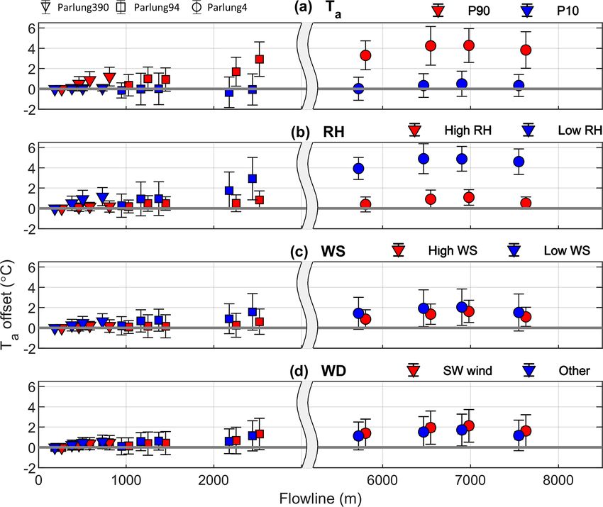
602                                                                       T. E. Shaw et al.: Distributed air temperature on mountain glaciers

Table 2. The details of each site where distributed on-glacier air temperatures are available. Elevation ranges and ERA5 mean summer air
temperatures (MSATs) are reported for the year of investigation. Precipitation totals (PT, mm) were obtained from the cited literature.

   Site                                          Latitude      Longitude            Year(s)        Elevation      MSATa            PT      Ta data reference
                                                                                                     m a.s.l.        ◦C           mm
   Parlung glaciers            (Tibet)             29.24           96.93       2018–2019         4600–5800           2.19        679       This Study
   CMBC                      (Canada)              50.32         −122.48       2006–2008         1375–2898          10.29       1113       Shea and Moore (2010)
   AVDM                          (Italy)           46.42           10.62       2010–2011         2650–3769           7.94      1233b       Carturan et al. (2015)
   Tsanteleina Glacier           (Italy)           45.48            7.06            2015         2800–3445          13.76        805       Shaw et al., (2017)
   Haut Glacier d’Arolla (Switzerland)             45.97            7.52            2010         2550–3520           7.28       1663       Ayala et al. (2015)
   McCall Glacier               (USA)              69.31         −143.85       2004–2014         1375–2365          −2.28        500       Troxler et al. (2020)
   Juncal Norte Glacier        (Chile)            −33.01          −70.09       2007–2008         2900–5910           6.58        352       Ayala et al. (2015)
   Greve Glacier               (Chile)            −48.88          −73.52       2015–2016            0–2400           −0.1      6450c       Bravo et al. (2019a)
   Pasterze Glacier          (Austria)             47.09           12.71            1994         2150–3465          12.66       2761       Greuell and Böhm (1998)
   Universidad Glacierd        (Chile)            −34.69          −70.33       2009–2010         2463–4543           8.24        474       Bravo et al. (2017)
   Peyto Glacierd            (Canada)              51.66         −116.55            2011         2260–3000           2.94        800       Pradhananga et al. (2020)
   Djankuat Glacierd          (Russia)             43.20           42.77            2017         3210–4000          12.13        950       Rets et al. (2019)
a MSAT corrected from ERA5 grid height to mean elevation of glacier using the environmental lapse rate. b Average for 1979–2009. Precipitation for 2010–2011 was above average at
∼ 1400 mm (Luca Carutran, personal communication, 2020). c Value taken from Bravo et al. (2019b). d Glaciers where the ELR was used to distribute temperature for k1/k2
calculation. See text for details.

Figure 3. The mean Ta against elevation and uncertainty (error bar) for (a) all hours (n = 3312) and (c) P90 h (n = 312). Panels (b) and (d)
are the equivalent plots against flowline distance. Coloured lines show the linear fit against elevation (lapse rate) to each glacier.

glacier flowline and extension of the katabatic wind into the                             for the entire dataset. For P90 conditions (Fig. 6a), differ-
pro-glacial area.                                                                         ences between Ta Amb and observed on-glacier temperatures
   The mean difference of along-flowline Ta and Ta Amb us-                                are up to 5.8 ◦ C at flowline distances greater than 7000 m.
ing the catchment lapse rate is shown in Fig. 6. For the                                  These differences appear to increase beyond 2000 m along
coolest 10 % of hours at AWS_Off (P10), there is gener-                                   the flowline (Parlung94), though significant differences can
ally minimal difference between Ta Amb and observed Ta                                    be witnessed for all glaciers (different symbols in Fig. 6).

The Cryosphere, 15, 595–614, 2021                                                                                    https://doi.org/10.5194/tc-15-595-2021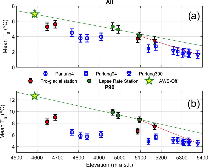
T. E. Shaw et al.: Distributed air temperature on mountain glaciers                                                                     603

Figure 4. The mean Ta against elevation for all hours (a) and P90 h (b), where blue markers are on-glacier T loggers, red markers are
pro-glacial T loggers and green circles denote off-glacier T loggers used to construct an hourly variable catchment lapse rate (green line),
extrapolated from AWS_Off (star). The red line indicates the piecewise lapse rate above the elevation of T 1390 to lapse Ta to the top of the
flowline. A 0.5 ◦ C uncertainty is shown by the error bar for each station (not applied to the lapse rate for neatness).

This is generally associated with drier conditions, and for              clear relation to the incoming shortwave radiation recorded
hours of greater relative humidity (AWS_Off), when con-                  at AWS_Off (correlations of 0.44, 0.60 and 0.80 for Par-
ditions are generally cooler, differences are unsurprisingly             lung390, Parlung94 and Parlung4, respectively), which is in-
smaller (Fig. 6b). Considering free-air wind variability pro-            dicative of warmer ambient conditions (i.e. P90). For Par-
vided by ERA5 reanalysis, Ta differences are largest for the             lung390 the maximum daily differences are much smaller,
dominant south-westerly wind direction (85 % of hours) and               though they vary considerably throughout the summer. For
when free-air wind speeds are smallest (Fig. 6c and d). How-             2019, maximum daily Ta offsets on Parlung390 steadily in-
ever, un-corrected, gridded wind speeds do not appropriately             crease during July and August and then fall close to zero in
represent the local free-air boundary conditions, and thus the           September. The maximum differences for Parlung4 and Par-
interaction of off-glacier wind speeds and the glacier bound-            lung94, however, remain sizeable (Fig. 7), perhaps due to the
ary layer development remains unclear for these glaciers. For            persistence of katabatic winds over a larger flowline distance
all but the coolest ambient temperatures (Fig. 6a), observa-             even under the relatively cooler conditions of September. Be-
tions at the greatest flowline distances deviate the most from           cause our study period focuses on the core monsoon period
the estimated values. Besides the analyses against individ-              (Yang et al., 2011), we do not observe the influence of mon-
ual meteorological variables, the differences are largest for            soon arrival or cessation on the Ta variability of the Parlung
warm/anticyclonic conditions and lowest for cool/cyclonic                glaciers.
conditions.
   The differences between Ta Amb and on-glacier Ta are                  5.3   Parameterisation of along-flowline air
highly variable in time, however, and related to the prevail-                  temperatures
ing conditions of a given year (Fig. 7). Considering the max-
imum daily Ta differences at the on-glacier T logger clos-
                                                                         Figure 8 presents the temperature sensitivities of the SM10
est to the terminus of each glacier (Table 1, Fig. 2), we find
                                                                         approach for the Parlung glaciers and available distributed
that Parlung94 and Parlung4 T loggers have similar magni-
                                                                         Ta datasets around the world (Table 2). Comparing the k1
tudes of Ta offsets during the mid-summer months, partic-
                                                                         and k2 parameters from Tibet to the parameters of Shea and
ularly for 2018 (Fig. 7). These maximum differences are in
                                                                         Moore (2010) from western Canada, a similar behaviour is

https://doi.org/10.5194/tc-15-595-2021                                                             The Cryosphere, 15, 595–614, 2021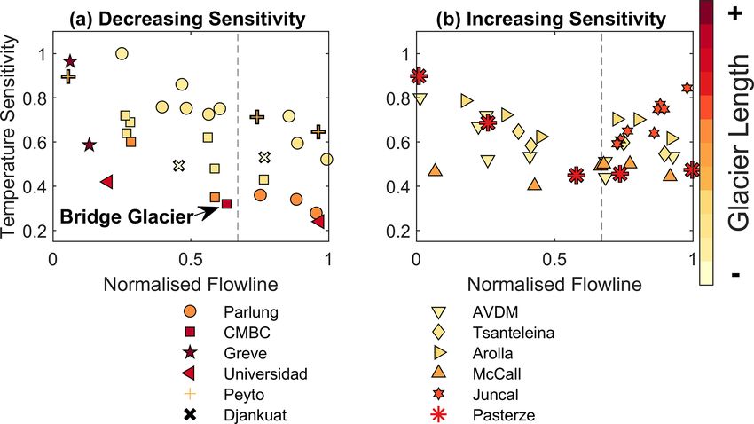
604                                                       T. E. Shaw et al.: Distributed air temperature on mountain glaciers

Figure 5. Estimated (Ta Amb) vs. observed Ta at each T -logger location (including off-glacier T loggers). Individual, hourly values are
coloured by the observed wind speeds at AWS_On (Parlung4). ∗ denotes stations that are off glacier.

observable up to ∼ 2000–3000 m of flowline distance (red              crease in temperature sensitivity at large flowline distances
and blue symbols). The exponential functions that are fitted          (∼ 10 000 m) previously only witnessed from one location
to the observations at Parlung glaciers and the original study        on Bridge Glacier, Canada (Shea and Moore, 2010). At these
are distinct (red and blue lines in Fig. 8, Table 3), although        stations, changes in on-glacier Ta are less than a third of the
within the confidence intervals of each other. Fitting an ex-         equivalent change in Ta Amb.
ponential function for all sites where a down-glacier decrease           Figure 9 shows the k2 parameters plotted against flowline
in temperature sensitivity (k2) is evident (black dashed line         distance, coloured by rankings of MSAT and precipitation to-
in Fig. 8b) clearly misrepresents many of the observations,           tals (Table 2). The warmest of the investigated sites (during
particularly those at greater flowline distances, balancing the       the measurement years) lie closer to the original SM10 ex-
behaviours reported for different sites.                              ponential function up to ∼ 4000 m, whereas deviation of the
   Notably, observations at McCall Glacier, Alaska, relate            k2 parameters from this line appears larger for the relatively
very well to ambient Ta under cooler conditions, with most            cold sites (Greve, McCall and Peyto – Fig. 9a). The main
k1 values remaining > 0.9. Above the T ∗ threshold, how-              exception to this is for Juncal Norte, which demonstrates a
ever, the relationship of observed and estimated Ta results           high and rapidly increasing sensitivity of ambient Ta at the
in increasing k2 along the flowline, in contradiction to the          greatest flowline distances.
majority of the other datasets. Nevertheless, these data also            No clear patterns are visible in relation to mean annual
confirm the increased temperature sensitivity on the glacier          precipitation, though the distinct behaviour at Juncal Norte
terminus (Troxler et al., 2020) as evident with datasets for          Glacier corresponds to the driest of the study sites considered
Tsanteleina (Shaw et al., 2017), Arolla and Juncal Norte              (Fig. 9b).
(Ayala et al., 2015). Observations at Parlung4 and Univer-               A clear difference between the station observations of
sidad Glacier (Bravo et al., 2017) emphasise the strong de-           Shea and Moore (2010) and Parlung glaciers at large flowline

The Cryosphere, 15, 595–614, 2021                                                           https://doi.org/10.5194/tc-15-595-2021
T. E. Shaw et al.: Distributed air temperature on mountain glaciers                                                                     605

Figure 6. The mean and standard deviation (error bars) of hourly Ta differences (Ta Amb – observed) along the glacier flowline. Each panel
depicts hourly grouping by (a) off-glacier Ta at AWS_Off (P90 is ≥ 10.5 ◦ C and P10 is ≤ 3.5 ◦ C), (b) off-glacier RH at AWS_Off (high is
> 90 % and low is < 70 %), (c) wind speed from ERA5 (high is > 2.5 m s−1 and low is < 0.7 m s−1 ) and (d) dominant wind direction from
ERA5 (south-west wind direction is considered as 180–270◦ ). Marker shapes show the different glaciers, as in Figs. 3 and 4. X axes are split
to improve visibility at low flowline distances.

Table 3. The coefficients of the original SM10 model and those fitted to the k1 and k2 sensitivities on the Parlung glaciers and all glaciers
where no warming effect was evident (see Fig. 10).

     Model                         k1 = β1 × exp(β2 × DF)                                  k2 = β3 + β4 × exp(−β5 × DF)
     CMBC (Shea and Moore,         β1 = 0.977                                              β3 = 0.29
     2010)                         β2 = −4.4 × 10⁻⁵                                        β4 = 0.71
                                                                                           β5 = 5.6 × 10⁻³
     Parlung                       β1 = 0.894 (0.805, 0.983)                               β3 = 0.349 (0.241, 0.456)
                                   β2 = −2.972×10⁻⁵ (−5.543×10⁻⁵ , −4.0×10⁻⁶ )             β4 = 0.624 (0.492, 0.757)
                                                                                           β5 = 4.4 × 10⁻³ (1.7 × 10⁻⁴ , 7.2 × 10⁻⁴ )
     All (no increased sensitiv-   β1 = 0.923 (0.886, 0.96)                                β3 = 0.343 (0.225, 0.46)
     ity on glacier terminus)      β2 = −3.375×10⁻⁵ (−5.543×10⁻⁵ , −4.0×10⁻⁶ )             β4 = 0.511 (0.38, 0.642)
                                                                                           β5 = 4.2 × 10⁻³ (1.5 × 10⁻⁴ , 6.9 × 10⁻⁴ )

distances (Fig. 8) is the total distance of that station observa-        only ∼ 60 % of the total glacier length (Bridge Glacier –
tion from the glacier terminus, which suggests a possible dif-           CMBC), neither representing the smallest temperature sensi-
ference in processes occurring between sites. Accordingly,               tivity (Fig. 8b), nor an increasing temperature sensitivity wit-
we plot the k2 parameters as a function of the normalised                nessed at the terminus of the glacier (and estimated using the
flowline (Fig. 9c and d), adjusted by the total length of glacier        ModGB model) by other studies (Ayala et al., 2015; Troxler
for the year(s) of observation (Table 2). The largest flowline           et al., 2020). We group glaciers by the presence (or absence)
distance observation of the entire dataset (Fig. 9a) extends             of an increasing temperature sensitivity on the terminus in

https://doi.org/10.5194/tc-15-595-2021                                                             The Cryosphere, 15, 595–614, 2021
606 T. E. Shaw et al.: Distributed air temperature on mountain glaciers
Figure 7. Maximum daily Ta differences (Ta Amb – observed) at the T logger closest to the terminus on each glacier for 2018 (a, b) and
2019 (c, d). Maximum daily Ta differences are plotted against mean daily incoming shortwave radiation (SWin) at AWS_Off in panels (b)
and (d).
Fig. 10. We find that there is no clear relation between the et al., 2010; Immerzeel et al., 2014; Gabbi et al., 2014; Hey-
total length of the glacier and increasing temperature sen- nen et al., 2016; Jobst et al., 2016). Despite this, the lack
sitivity, which is seen for both smaller and larger glaciers of locally available observations often requires modellers to
(Fig. 10b). For those glaciers where a temperature sensitiv- force models with the nearest off-glacier record of Ta and
ity increase (a relative ModGB warming effect – Fig. 1a) is extrapolate it based upon the ELR value as a default. In the
evident, it is found only on the lowest 30 % of the glacier case of Tibetan glaciers, model studies have often derived
terminus (Fig. 10b – vertical dashed line). static lapse rates between on- and off-glacier stations (Huin-
tjes et al., 2015) or downscale Ta with a correction factor
based upon a single on-glacier location (e.g. Caidong and
6 Discussion Sorteberg, 2010; Yang et al., 2013; Zhao et al., 2014). To
the authors’ knowledge, this is the first time that such de-
6.1 Relevance of the findings from Parlung glaciers tailed information regarding spatio-temporal variations in Ta
has been presented for a glacier of the Tibetan Plateau. Be-
Our observations of along-flowline Ta on the glaciers in the
cause glaciers of the south-eastern Tibetan Plateau have been
Parlung catchment provide more evidence of the spatial vari-
shown to be particularly susceptible to increases in Ta (Wang
ability of the glacier cooling and dampening effect (Oerle-
et al., 2019), accurately parameterising Ta along glaciers of
mans, 2001; Carturan et al., 2015; Shaw et al., 2017) and
differing size is highly relevant for present and future melt
highlight the need to appropriately estimate its behaviour for
modelling attempts. This is especially true where glaciers
use in glacier energy balance and enhanced temperature in-
begin to shrink or fragment (Munro and Marosz-Wantuch,
dex melt models (Petersen and Pellicciotti, 2011; Shaw et al.,
2009; Jiskoot and Mueller, 2012; Carturan et al., 2015) and
2017; Bravo et al., 2019a). It has long been observed that a
become more sensitive to ambient air temperatures due to a
static lapse rate is inappropriate for characterising the spatio-
lack of katabatic boundary layer development (Figs. 6 and 7).
temporal variability of Ta , both within the KBL (Greuell
The summer monsoon exerts a strong control on the en-
et al., 1997; Konya et al., 2007; Marshall et al., 2007; Gard-
ergy and mass balance of Tibetan glaciers (Yang et al., 2011;
ner et al., 2009; Petersen and Pellicciotti, 2011) and out-
Mölg et al., 2012; Zhu et al., 2015). Although our dataset
side the glacier boundary layer in adjacent valleys (Minder
The Cryosphere, 15, 595–614, 2021 https://doi.org/10.5194/tc-15-595-2021T. E. Shaw et al.: Distributed air temperature on mountain glaciers 607
Figure 8. The calculated k1 and k2 sensitivities as a function of the flowline distance of each observation on the Parlung glaciers (red circles)
and other global datasets (Table 2). The dashed blue and red lines show the fitted exponential parameterisation of Shea and Moore (2010)
and this study, respectively. The dashed black line and shaded area denote the equivalent parameterisation for all observations without a large
increase in sensitivity on the glacier terminus (warming effect – explicitly excluding data from McCall, Juncal Norte and Djankuat). The
shaded area represents the 95 % confidence interval of this fit line.
spanned two summers of only the core monsoon period for 6.2 Parameterising glacier temperature sensitivity
this region (Yang et al., 2011), we have shown that the sensi-
tivity of the glacier to external temperature changes (shown
by on-glacier and ambient Ta differences) has a sizeable In this study, we discuss the temperature sensitivity of on-
temporal variability that can be controlled by the monsoon glacier Ta based upon observations above a threshold ambi-
weather conditions (such as ambient air temperature, humid- ent temperature for the onset of katabatic conditions (T ∗ ).
ity and incoming radiation) and can sometimes be indepen- This sensitivity to ambient temperature during relatively
dent of the glacier size (Fig. 7). Whilst we cannot determine warm conditions, indicated by the k2 parameter of Shea
the impact of monsoon timing and intensity upon the tem- and Moore (2010) (Fig. 1), demonstrates a generally consis-
perature sensitivity of these glaciers with the current dataset, tent behaviour between the T -logger observations of Parlung
we are able to determine that the observed relationship to glaciers and those where this model had been previously im-
flowline distance is consistent with that of other regions of plemented (Shea and Moore, 2010; Carturan et al., 2015).
the world (Fig. 8). Future work on Tibetan glaciers should While data from the Parlung catchment provide an impor-
attempt to extend monitoring to the pre-monsoon period to tant confirmation of the temperature sensitivity for some Ti-
identify if a seasonal onset for the changing glacier tempera- betan glaciers, further studies of individual glaciers can pro-
ture sensitivity can be defined and how the monsoon may af- vide only local parameterisations for temperature sensitivity
fect it. Particular focus should be given to understanding the that may not be applicable to other sites. Accordingly, we
local meteorological conditions for each glacier, as this may have made here one of the first attempts at combining many
explain some of the variability in Ta offset values and why of the published datasets regarding distributed Ta on moun-
they may sometimes be independent of the along-flowline tain glaciers around the world (Table 2) to examine the po-
distance (Fig. 7). tential transferability of a model accounting for temperature
sensitivity (Fig. 8).
We found a sizeable spread in the temperature sensitiv-
ities of Ta for the on-glacier datasets considered, though a
https://doi.org/10.5194/tc-15-595-2021 The Cryosphere, 15, 595–614, 2021608 T. E. Shaw et al.: Distributed air temperature on mountain glaciers Figure 9. The k2 sensitivities as a function of flowline distance (a, b) and a normalised distance, considering the total flowline distance for the year of study (c, d). The individual glaciers of grouped studies (Parlung, CMBC and AVDM) are separated and normalised by the individual glacier length (symbols as in Fig. 8). Glaciers are coloured by rankings of the mean summer air temperatures (MSAT – a and c) and precipitation total (b, d). The original SM10 parameterisation is retained in (a) and (b). Figure 10. The k2 sensitivity along the normalised flowline compared to total glacier length (colour bar). Glaciers have been grouped in two clusters: (a) those with down-glacier decreasing sensitivity, and (b) those with increasing sensitivity towards the glacier terminus. consistently rapid decrease in sensitivity along glacier flow- flect a 0.7–0.8 sensitivity to changes in Ta Amb. Beyond this lines is found for most sites up until ∼ 2000–3000 m of dis- distance, the temperature sensitivities notably follow one of tance (Fig. 8b). While localised meteorological and topo- two patterns: a continued albeit less rapid decrease in sen- graphic factors likely interact to explain the spread of sensi- sitivity (generally following the model proposed by Shea tivities at small flowline distances (Fig. 8b), the results sug- and Moore, 2010) or a tendency toward increasing sensitiv- gest that small glaciers with flow lengths < 1000 m would re- ity at the largest flowline distances (in agreement with the The Cryosphere, 15, 595–614, 2021 https://doi.org/10.5194/tc-15-595-2021
T. E. Shaw et al.: Distributed air temperature on mountain glaciers                                                              609

ModGB model – Fig. 1a). With reference to the relative Ta           ture sensitivity begin at ∼ 70 % of the total flowline distance
differences among only on-glacier observations, these have          (Fig. 10). A smaller temperature sensitivity can be observed
been termed as down-glacier “cooling” or “warming”, re-             for larger glaciers (Fig. 10a), which is consistent with the de-
spectively, in many past studies (Ayala et al., 2015; Carturan      velopment of the KBL over a large fetch (Greuell and Böhm,
et al., 2015; Shaw et al., 2017; Troxler et al., 2020). Whilst      1998; Shea and Moore, 2010), though the length itself indi-
the former is generally associated with relatively warmer re-       cates nothing clear about why greater temperature sensitivity
gions of study (Fig. 9), such as the southern Coast Mountains       exists for some glacier termini (Fig. 10b).
(Shea and Moore, 2010) or Universidad Glacier (Bravo et al.,           The clear outlier of these datasets is Juncal Norte Glacier
2017), no strong relationship of the climate setting exists be-     in Chile (Fig. 8b). It is interesting to note that Juncal Norte is
tween these sites to explain the magnitude of the tempera-          the only reported case in the literature on Ta variability where
ture sensitivity (i.e. the strength of the glacier cooling and      the warmest hours of the afternoon correspond to the dom-
dampening effect) or the observed increases in temperature          inance of an up-valley, off-glacier wind (Pellicciotti et al.,
sensitivity on glacier termini (Ayala et al., 2015; Shaw et al.,    2008; Petersen and Pellicciotti, 2011). Counter to the typi-
2017; Troxler et al., 2020).                                        cal role of the dominant, down-glacier wind layer for these
   Interestingly, we noted that the station with the largest        warmest afternoon hours (Greuell et al., 1997; Greuell and
flowline distance used to derive the parameterisation by Shea       Böhm, 1998; Strasser et al., 2004; Jiskoot and Mueller, 2012;
and Moore (2010) was located at only around 60 % of the             Shaw et al., 2017; Troxler et al., 2020), up-valley winds on
total glacier flowline distance (Bridge Glacier – Fig. 10),         Juncal Norte seemingly erode the along-flowline reduction in
whereas data presented by other studies provided observa-           temperature sensitivity (along-flowline cooling) up to a dis-
tions up to the glacier terminus (Greuell and Böhm, 1998;           tance along the flowline where it is theoretically at its maxi-
Ayala et al., 2015; Shaw et al., 2017; Troxler et al., 2020),       mum (point 3 in Fig. 1). Evidence from other glaciers suggest
therefore potentially parameterising different effects of the       that this point is close to upper observations for Juncal Norte
glacier boundary layer. It has been suggested that obser-           at ∼ 70 % of the total flowline (Fig. 10b), though further ob-
vations at large flowline distances (such as those on Par-          servations on Juncal Norte Glacier would be required to test
lung4 or Bridge Glacier) represent a segment of the boundary        this.
layer where the near-surface layer becomes highly insensi-             Finally, the extent to which a glacier terminus is con-
tive to the ambient free-air temperature fluctuations (point 3      strained by high valley slopes may be an additional explana-
in Fig. 1a and d). This phenomenon has been shown to be             tory factor for the occurrence of increasing temperature sen-
sustained over large fetch distances by an increasing depth         sitivities on some glaciers (Fig. 10). While this may limit
of the glacier wind layer (van den Broeke, 1997; Greuell and        the suggested boundary layer divergence (Munro, 2006), it
Böhm, 1998; Shea and Moore, 2010; Jiskoot and Mueller,              may equally promote greater warming due longwave emis-
2012). However, as air parcels travel down glacier toward the       sion from valley slopes (e.g. Strasser et al., 2004; Ayala et al.,
glacier terminus (point 4 in Fig. 1a and d), they potentially       2015). We calculated the terminus width/length ratio of each
encounter warm-air entrainment due to a divergent bound-            glacier and compared it to the presence of increasing temper-
ary layer (Munro, 2006), up-valley winds (Pellicciotti et al.,      ature sensitivity on the terminus (Fig. S4 in the Supplement),
2008; Oerlemans, 2010; Petersen and Pellicciotti, 2011),            revealing a potential relationship between the two. However,
large changes in surface slope and the dominance of adia-           given the available data for this study and the unknown ex-
batic heating over sensible heat losses (Greuell and Böhm,          tent to which longwave emission may affect a fast-moving
1998), or heating from debris-covered ice at the terminus           air parcel (Ayala et al., 2015), a dedicated study would be
(Brock et al., 2010; Shaw et al., 2016; Steiner and Pellic-         required to further address this hypothesis.
ciotti, 2016; Bonekamp et al., 2020). These are effects of
the glacier boundary layer that the ModGB model was de-             6.3   Future directions for researching air temperatures
signed to account for, though we did not explicitly test this             on glaciers
within our study due to a requirement for more data and a
greater number of parameters and assumptions (Shaw et al.,          A limitation of our work is the dependency of the derived
2017). The strength of this so called along-glacier warming         global temperature sensitivities (Fig. 8b) to the available off-
effect could therefore be governed by local topography (ad-         glacier data and the published lapse rates to extrapolate them
justing the boundary layer convergence or divergence) or the        to the relevant elevations on glacier. In our case, we are
total glacier flowline distance and the large fetch of a cool air   able to identify a potentially non-linear lapse rate of Ta Amb
parcel overcoming the competing effect of warm, up-valley           for the highest elevations over Parlung94 and Parlung390
winds (Fig. 1d – as seen at T 24 in Fig. 5).                        (Fig. 4). Although we cannot confirm this without off-glacier
   By grouping glaciers by the presence of the observed in-         observations above the top of the flowline (Carturan et al.,
crease in temperature sensitivity and normalising the flowline      2015), we are able to well constrain ambient air temperature
distance of the observations by the total flowline for each         distribution using hourly observations at several off-glacier
glacier, we identify that the relative increases in tempera-        locations to derive the best possible catchment lapse rate.

https://doi.org/10.5194/tc-15-595-2021                                                       The Cryosphere, 15, 595–614, 2021
610                                                      T. E. Shaw et al.: Distributed air temperature on mountain glaciers

For other datasets (Table 2), we rely upon the available off-       what the direct comparison of the temperature sensitivity pre-
glacier data and lapse rates that are not derived in a consis-      sented here and the “climatic sensitivity” of previous works.
tent manner. The derivation of flowline distances from the             We consider the SM10 approach and the use of k2 to be an
DEM is also not consistent between the prior studies (Shea          appropriate indicator of temperature sensitivity for mountain
and Moore, 2010; Carturan et al., 2015; Shaw et al., 2017;          glaciers in future work of this type. This approach is an eas-
Bravo et al., 2019a; Troxler et al., 2020) and may hold some        ily adaptable method for calculating glacier temperature sen-
small influence on the derived parameterisations (Table 3),         sitivity and thus estimating on-glacier Ta . However, the com-
particularly at lateral locations on the glacier (not explored      peting effects of glacier katabatic and up-valley winds/debris
here), which can be subject to different micro-meteorological       or valley warming need to be incorporated to address the
effects (van de Wal et al., 1992; Hannah et al., 2000; Shaw         challenges that less simplistic methods (i.e. ModGB) were
et al., 2017). Equally, the uncertainty of the actual observa-      designed for.
tions (e.g. Sect. 3.2) is hard to clearly define due the variable      Based upon the findings of this work, we recommend that
instrumentation (sensors and radiation shielding), on-glacier       future research (i) attempt to standardise, where possible, the
location, and local topographic and micro-meteorological ef-        measurement and comparison of off- and on-glacier air tem-
fects of each study site (Table 2). Because our study, and          perature, exploring the use of artificially ventilated radiation
many similar studies of this kind, did not have artificially        shields that are less prone to heating errors (Georges and
ventilated radiation shields available, the uncertainty of the      Kaser, 2002; Carturan et al., 2015), (ii) instrument glaciers
measured Ta is difficult to quantify. We consider this to be        of varying size in the same catchment to explore the relative
less problematic at large flowline distances, where good ven-       importance of glacier size and local meteorological condi-
tilation to the sensors is often provided by the glacier kata-      tions (Fig. 7), and (iii) model the detailed interactions of air
batic wind layer even under warm conditions. However, at            flows on glacier termini using, for example, large eddy sim-
short flowline distances in the glacier accumulation zones,         ulations (Sauter and Galos, 2016; Bonekamp et al., 2020) in
uncertainty of both the on-glacier observations and ambi-           order to identify possible drivers of the observed increase in
ent Ta extrapolation is larger. Artificially ventilated radiation   temperature sensitivity for certain glacier areas (point 4 in
shields are not commonplace in glaciological research due           Fig. 1).
to the additional power demands that often cannot be met
though would be strongly encouraged for further research
into the temperature sensitivity of mountain glaciers. Further      7    Conclusions
work on a unified model of estimating Ta should need to ad-
dress these issues, perhaps with further dedicated analyses.        We presented a new dataset of distributed on-glacier air tem-
   In our study, we apply the parameterisation of Carturan          peratures for three glaciers of different size in the south-east
et al. (2015) to derive along-flowline values of the theoretical    Tibetan Plateau during two summers (July–September). We
onset of the KBL (T ∗ ). While these values appear appropri-        analysed the along-flowline air temperature distribution for
ate for our case studies (based upon manual inspection), they       all three glaciers and compared them to the estimated ambi-
were derived for a smaller sample size of total observations.       ent temperatures derived from several local off-glacier sta-
We experimented with a static T ∗ value of 5 ◦ C in order to        tions. Using this information, we parameterised the along-
test the sensitivity of our analysis to the assumptions of T ∗ ,    flowline temperature sensitivities of these glaciers using the
though we found negligible sensitivity of derived k2 on T ∗         method proposed by Shea and Moore (2010) and presented
(not shown). Similarly, a sensitivity to the choice of constant     the results in the context of several available distributed on-
lapse rate for those sites without available lapse rate infor-      glacier datasets. The key findings of this work are the follow-
mation (Table 2) proved to have only a small influence on           ing.
the derived k1 and k2 values.
   Finally, in this study we assess temperature sensitivity             1. For our Tibetan case study, on-glacier air tempera-
based upon ambient air temperatures above the T ∗ thresh-                  tures at short flowline distances display a high tempera-
old. This is partly different from the “climatic sensitivity”              ture sensitivity (i.e. demonstrate a relationship with off-
presented by earlier works (Greuell et al., 1997; Greuell and              glacier air temperature that is close to 1). We therefore
Böhm, 1998; Oerlemans, 2001, 2010), which considered an                    confirm earlier evidence regarding the high tempera-
all-hour temperature sensitivity value (i.e. not thresholding              ture sensitivity of high-elevation, small glaciers (flow-
sensitivities by katabatic wind onset – Fig. 1b). However, ig-             line distances < 1000 m) to external climate and thus
noring the differences in temperature sensitivity before and               future warming.
after the onset of the KBL (Figs. 1c and 5) is arguably
an over-simplification and does not enable one to correctly             2. The largest differences between observed on-glacier and
describe the observed behaviours (Shea and Moore, 2010;                    estimated off-glacier air temperatures are found for the
Jiskoot and Mueller, 2012). Accordingly, we caution some-                  warmest off-glacier hours during drier, clear-sky condi-
                                                                           tions of the summer monsoon period.

The Cryosphere, 15, 595–614, 2021                                                          https://doi.org/10.5194/tc-15-595-2021
You can also read