Simulated Estuary-Wide Response of Seagrass (Zostera marina) to Future Scenarios of Temperature and Sea Level - Frontiers
←
→
Page content transcription
If your browser does not render page correctly, please read the page content below

ORIGINAL RESEARCH
                                                                                                                                             published: 21 October 2020
                                                                                                                                       doi: 10.3389/fmars.2020.539946

                                            Simulated Estuary-Wide Response of
                                            Seagrass (Zostera marina) to Future
                                            Scenarios of Temperature and Sea
                                            Level
                                            Cara R. Scalpone 1* , Jessie C. Jarvis 2 , James M. Vasslides 3 , Jeremy M. Testa 4 and
                                            Neil K. Ganju 5
                                            1
                                              Pitzer College, Claremont, CA, United States, 2 Department of Biology and Marine Biology, University of North Carolina
                                            Wilmington, Wilmington, NC, United States, 3 Barnegat Bay Partnership, Toms River, NJ, United States, 4 Chesapeake
                                            Biological Laboratory, University of Maryland Center for Environmental Science, Solomons, MD, United States,
                                            5
                                              US Geological Survey Marine Science Center, Woods Hole, MA, United States

                                            Seagrass communities are a vital component of estuarine ecosystems, but are
                                            threatened by projected sea level rise (SLR) and temperature increases with climate
                                            change. To understand these potential effects, we developed a spatially explicit model
                                            that represents seagrass (Zostera marina) habitat and estuary-wide productivity for
                                            Barnegat Bay-Little Egg Harbor (BB-LEH) in New Jersey, United States. Our modeling
                              Edited by:
                     Iris Eline Hendriks,
                                            approach included an offline coupling of a numerical seagrass biomass model with
     University of the Balearic Islands,    the spatially variable environmental conditions from a hydrodynamic model to calculate
                                   Spain
                                            above and belowground biomass at each grid cell of the hydrodynamic model
                      Reviewed by:
                                            domain. Once calibrated to represent present day seagrass habitat and estuary-wide
              Megan Irene Saunders,
   Oceans and Atmosphere (CSIRO),           annual productivity, we applied combinations of increasing air temperature and sea
                             Australia      level following regionally specific climate change projections, enabling analysis of the
                      Guillem Chust,
Technological Center Expert in Marine
                                            individual and combined impacts of these variables on seagrass biomass and spatial
   and Food Innovation (AZTI), Spain        coverage. Under the SLR scenarios, the current model domain boundaries were
                  *Correspondence:          maintained, as the land surrounding BB-LEH is unlikely to shift significantly in the future.
                    Cara R. Scalpone
                                            SLR caused habitat extent to decrease dramatically, pushing seagrass beds toward
               crscalpone@gmail.com
                                            the coastline with increasing depth, with a 100% loss of habitat by the maximum
                   Specialty section:       SLR scenario. The dramatic loss of seagrass habitat under SLR was in part due to
         This article was submitted to
                                            the assumption that surrounding land would not be inundated, as the model did not
Global Change and the Future Ocean,
               a section of the journal     allow for habitat expansion outside the current boundaries of the bay. Temperature
          Frontiers in Marine Science       increases slightly elevated the rate of summer die-off and decreased habitat area only
          Received: 03 March 2020           under the highest temperature increase scenarios. In combined scenarios, the effects
      Accepted: 28 September 2020
        Published: 21 October 2020
                                            of SLR far outweighed the effects of temperature increase. Sensitivity analysis of the
                               Citation:
                                            model revealed the greatest sensitivity to changes in parameters affecting light limitation
               Scalpone CR, Jarvis JC,      and seagrass mortality, but no sensitivity to changes in nutrient limitation constants.
Vasslides JM, Testa JM and Ganju NK
                                            The high vulnerability of seagrass in the bay to SLR exceeded that demonstrated for
       (2020) Simulated Estuary-Wide
       Response of Seagrass (Zostera        other systems, highlighting the importance of site- and region-specific assessments of
           marina) to Future Scenarios      estuaries under climate change.
        of Temperature and Sea Level.
             Front. Mar. Sci. 7:539946.     Keywords: seagrass (Zostera), climate change, spatial model, sea level rise, temperature, North American
    doi: 10.3389/fmars.2020.539946          Atlantic Coast, regional, eelgrass (Zostera marina)

Frontiers in Marine Science | www.frontiersin.org                                  1                                           October 2020 | Volume 7 | Article 539946
Scalpone et al.                                                                                                Seagrass Sensitivity to Future Climate

INTRODUCTION                                                               biomass models for seagrass deterministically calculate seagrass
                                                                           properties, such as shoot density or length, with equations that
Seagrass meadows are prevalent in estuarine ecosystems along               represent the empirically determined physiological relationships
continental coastlines around the globe and play a substantial             between environmental conditions and seagrass (Duarte, 1991;
role in ecosystem structure and functioning (Short et al.,                 Madden and Kemp, 1996; Zharova et al., 2001). Strict light
2007; Schmidt et al., 2011; Nordlund et al., 2016). Seagrass               requirements for growth allow seagrass habitat availability to be
meadows mitigate coastal erosion and help shape estuaries by               roughly predicted by an inversely proportional relationship with
trapping sediment, altering currents, and attenuating waves                water depth (Dennison, 1987; Duarte, 1991; Duarte et al., 2007).
(Fonseca and Fisher, 1986; Bos et al., 2007; Nordlund et al.,              Water temperature is often included in equations modeling
2016). As the prominent primary producer in many shallow                   seagrass rates of respiration, primary production, and mortality
coastal estuaries, seagrass moderates nitrogen and carbon cycling,         (Madden and Kemp, 1996; Cerco and Moore, 2001). More
while sequestering carbon over annual and longer timescales                complex seagrass biomass modeling approaches have included
(Short et al., 2007; Schmidt et al., 2011; Fourqurean et al.,              the impacts of other contributors to light attenuation, such as
2012). Furthermore, seagrass meadows provide essential habitat             epiphytic algae and phytoplankton (Madden and Kemp, 1996;
and food sources to other species, including many listed as                Plus et al., 2003). While more complicated ecological models
threatened or endangered (Hughes et al., 2009). Because of                 create more realistic scenarios, perhaps closer to replicating
the importance of seagrass in biological, physical, and chemical           reality, additional parameters can lead to greater sources of error
coastal processes, the health of a seagrass meadow can be used             in model prediction (Ganju et al., 2016). Numerical biomass
as a biological indicator of overall estuary health (Hughes et al.,        models are often one-dimensional (Madden and Kemp, 1996;
2009). However, seagrass communities are declining in many                 Kenov et al., 2013; Jarvis et al., 2014), but the development of
regions, including the Atlantic coast of North America, largely            spatially explicit models has expanded their use by incorporating
due to anthropogenic influences of human development and                   spatially variable environmental conditions and dynamics to
eutrophication (Orth et al., 2006; Waycott et al., 2009). Further          describe seagrass habitat and growth across ecosystems (Cerco
stress from anthropogenic climate change threatens seagrass                and Moore, 2001; Baird et al., 2016; DeAngelis and Yurek, 2017).
populations, with cascading effects throughout shallow coastal             Spatial distributions of seagrass are also modeled using species
ecosystems (McGlathery et al., 2013; Ondiviela et al., 2014).              distribution models (SDMs), a statistical method which relies
    Because seagrass species are both essential components                 on the cooccurrence of seagrass habitat with environmental
of shallow coastal ecosystems and particularly sensitive to                conditions for prediction rather than physiological biomass
environmental change, understanding the impacts of climate                 production equations (Saunders et al., 2014; Valle et al., 2014;
change on seagrass habitat is crucial for developing targeted              Wilson and Lotze, 2019).
conservation strategies (Kenworthy et al., 2007; Unsworth                      Both one-dimensional and spatially explicit seagrass models
et al., 2019). Ongoing temperature increases and sea level                 have been used to study the effects of environmental changes on
rise (SLR) due to climate change will alter both the thermal               seagrass habitat and growth (Carr et al., 2012; Jarvis et al., 2014;
and light environment in estuarine ecosystems, both of which               Davis et al., 2016). Used in this way, models provide a conceptual
are important factors for seagrass viability. Multiple properties          setting to test various environmental scenarios in ways that
(e.g., algal cells, colored dissolved organic matter, sediments)           a tradition experimental setting would not allow. Modifying
attenuate light as it travels through the water column to the              the light climate has been the focus of many spatially explicit
canopy of a seagrass meadow, limiting the photosynthetically               modeling studies, exploring the effects of suspended sediments
active radiation available for primary productivity (Ganju et al.,         (Saunders et al., 2017), eutrophication (Cerco and Moore, 2001;
2014). Seagrass species require greater light availability than most       del Barrio et al., 2014), and SLR (Carr et al., 2012; Saunders
other submerged primary producers, making them especially                  et al., 2013; Davis et al., 2016). Regardless of the mechanism
sensitive to changes in water depth and quality (Duarte,                   causing changes to light climate, studies agree that improvements
1991). Temperature conditions also limit seagrass growth, with             to light climate can expand habitat availability, whereas increased
species-specific critical temperatures for germination, an optimal         light limitation shrinks available habitat. Depending on the
temperature for growth, increased respiration with higher                  characteristics of a given ecosystem, however, SLR could also lead
temperatures, and a sensitivity to extreme heat stress (Evans              to habitat expansion if newly inundated areas become available
et al., 1986; Moore and Jarvis, 2008; Moore et al., 2012; Repolho          for colonization (Saunders et al., 2013; Valle et al., 2014).
et al., 2017). Temperature and depth have been shown to interact               The impacts of increasing temperatures on seagrass growth
to control seagrass survival, with higher light requirements               have primarily been explored using either one-dimensional
at higher temperatures to balance photosynthetic productivity              biomass models or regionally scaled SDMs with varying effects
with increased respiration (Tanaka and Nakaoka, 2007), and                 based on geographical location and the thermal preference of the
optimal resilience to marine heat waves at moderate depths                 studied seagrass species. Research using one-dimensional
(Aoki et al., 2020).                                                       numerical models have demonstrated that exposure to
    The strong dependence of seagrass growth on environmental              temperatures above the optimal temperature for growth can
conditions enables the development of seagrass biomass                     produce a net decrease in biomass, simulating the physiological
models, providing a theoretical setting to explore seagrass                tradeoff of reducing photosynthesis rates and increasing
responses to environmental change (Winsberg, 2003). Numerical              respiration rates as temperature rises (Marsh et al., 1986;

Frontiers in Marine Science | www.frontiersin.org                      2                                    October 2020 | Volume 7 | Article 539946
Scalpone et al.                                                                                                Seagrass Sensitivity to Future Climate

Jarvis et al., 2014). Studies employing SDMs have projected that           coastline (Figure 1; Kennish et al., 2013). Two barrier islands—
increases in temperature will have significant impacts to the              Island Beach and Long Beach Island—separate the bay from
geographic range of seagrass habitat, with possible extinctions            the Atlantic Ocean. Three inlets connect BB-LEH to the open
at latitudinal locations where seagrass are already near their             ocean: Point Pleasant Canal (via Manasquan Inlet), Barnegat
temperature maximum and expansion into locations which were                Inlet, and Little Egg Inlet (north to south respectively). Average
previously below their thermal range (Wilson and Lotze, 2019).             depth of the bay is 1.5 m, ranging down to 7 m in the channel
While both methods inform our understanding of the effects of              of Little Egg Harbor (Kennish, 2001). The tidal range attenuates
rising temperature on seagrass, one-dimensional biomass models             significantly with increased distance from the inlets, from 1 m at
do not capture ecosystem-scale dynamics, whereas SDMs cannot               Barnegat Inlet and Little Egg Inlet down to 0.2 m across a 5 m
describe physiological growth dynamics. Estuary-wide impacts               distance (Defne and Ganju, 2015). There are two seagrass species
of rising temperatures on seagrass growth and habitat availability         found within the bay—Zostera marina (eelgrass) and Ruppia
have not been studied, and furthermore, the impacts of SLR                 maritima (widgeon grass). Z. marina is the historically dominant
compounded with increased temperature across an estuarine                  species, found in the central and southern portions of the bay
ecosystem has not been explored.                                           (Kennish et al., 2013). R. maritima is present in the northern
    In this study, we aim to describe the sensitivity of seagrass          portion of the bay, north of Toms River (Kennish et al., 2013).
production and habitat suitability to temperature increases                The two seagrass species have differing ranges in appropriate
and SLR across an estuarine ecosystem using a simple,                      habitat, as R. maritima is the more tolerant species to variation
spatially explicit biomass model. Our modeling approach                    in environmental conditions and can survive in mesohaline as
quantifies habitat suitability by applying spatially variable              well as polyhaline conditions (Wetzel and Penhale, 1983; Evans
physical parameters from a three-dimensional hydrodynamic                  et al., 1986; Short et al., 2007). Z. marina habitat along the North
model to a seagrass productivity point model, coupled off-                 American Atlantic coast ranges geographically from Greenland
line with no-feedback (Madden and Kemp, 1996; Defne and                    to North Carolina, with a maximum depth of 12 m observed
Ganju, 2015, 2018; Straub et al., 2015). We implemented                    in clear water near the northern range limit (Short et al., 2007;
scenarios of variable temperature and sea level to test their              Wilson and Lotze, 2019). In BB-LEH, seagrass meadows are
separate and combined impacts on seagrass habitat suitability and          found predominantly at depths less than 1 m along the sandy
productivity, and performed sensitivity analyses to explore model          shoals (Kennish, 2001), although Z. marina has been observed
behavior. Our model was calibrated to simulate Zostera marina              down to 4.6 m (see section “Calibration Results”; Lathrop and
meadows in Barnegat Bay-Little Egg Harbor (BB-LEH) estuary in              Haag, 2011; Defne and Ganju, 2015). Depth is a significant
New Jersey. Z. marina is the primary seagrass species in North             control on seagrass habitat viability in BB-LEH due to high light
American Atlantic estuaries, which are particularly vulnerable             attenuation, with meadows below 1 m becoming increasingly
to SLR as the North American Atlantic coast experiences SLR                sparse (Kennish et al., 2008; Ganju et al., 2014). In addition to
at a faster rate than the global average (Sallenger et al., 2012).         depth, seagrass habitat is negatively associated with substrates
Our simulations use climate change projections specific to the             with high organic matter, which are primarily found in deeper
North American Atlantic region (Collins et al., 2013; IPCC,                portions of the bay (Ocean County Soil Conservation District
2013), allowing our modeling to reflect the impacts of SLR                 [OCSCD] and the United States Department of Agriculture
and temperature increases that other mid-Atlantic estuaries                Natural Resources Conservation Service [USDA NRCS], 2005).
are expected to experience in the future. The resulting simple                 Over the past 30 years, there has been a documented decrease
spatial model for seagrass habitat and production provided an              in seagrass habitat extent and density in BB-LEH (Lathrop and
efficient method for assessing seagrass sensitivity to future change       Haag, 2011; Kennish et al., 2013). Prior work has attributed the
across the ecosystem.                                                      decrease in seagrass coverage to increased nutrient loading and
    Based on the physiological controls of temperature and light           eutrophication from the rapid development within the Barnegat
on seagrass growth, we hypothesized that SLR would act as a                Bay watershed (Lathrop and Conway, 2001). The estuary is
control to seagrass habitat extent by limiting light availability,         considered highly eutrophic (Bricker et al., 2007), with nutrient
until rising temperatures reached a threshold at which heat stress         loadings highest in the northern, more developed part of the
would cause early seagrass die-off. In our analysis, if SLR was            estuary (Pang et al., 2017). Frequent dredging and extensive
the leading control to seagrass habitat extent, we expected to see         shoreline hardening are also stressors on the ecosystem (Kennish,
seagrass habitat strictly follow depth gradients with increases in         2001). By 1999, 45% of the total shoreline length had been
sea level. If temperature was the leading control, we expected to          bulkheaded, and 70% of the upland shores were developed
see an overall decrease in biomass due to increasing respiration           (Lathrop and Bognar, 2001). In recent years, R. maritima has
losses and lower primary productivity at extreme temperatures.             begun to colonize seagrass beds in the central bay, mixing in with
                                                                           Z. marina as the density of Z. marina decreases (Barnegat Bay
                                                                           Partnership, 2016).
MATERIALS AND METHODS
                                                                           Analysis Overview
Site Description                                                           Our spatially explicit modeling approach began with a simplified
Barnegat Bay-Little Egg Harbor (BB-LEH) is a shallow, temperate            version of a biomass production model developed for
back-barrier estuary that stretches 68 km along the New Jersey             Z. marina growth in BB-LEH by Straub et al. (2015). The

Frontiers in Marine Science | www.frontiersin.org                      3                                    October 2020 | Volume 7 | Article 539946
Scalpone et al.                                                                                                              Seagrass Sensitivity to Future Climate

  FIGURE 1 | Bathymetry of Barnegat Bay-Little Egg Harbor (BB-LEH) estuary and observation sites used to develop the biomass production model in Straub et al.
  (2015), with Black outline showing the original computational domain of hydrodynamic model, and Pink outline marking the domain of the coupled
  production-hydrodynamic model.

biomass production model calculated daily aboveground and                           the Coupled-Ocean-Atmosphere-Wave-Sediment Transport
belowground biomass at specific locations when provided with                        (COAWST) modeling system. The coupled production-
water depth, ambient water temperature, photosynthetically                          hydrodynamic model was run for 1 year (May 1, 2012 to April
active radiation, and nitrogen availability. To establish the spatial               30, 2013) using environmental forcing functions from the
patterns of seagrass production in BB-LEH, we executed the                          hydrodynamic model run, the atmospheric model used to force
biomass production model at each computational grid cell                            the hydrodynamic model (North American Regional Reanalysis
of a hydrodynamic model that was previously configured for                          [NCEP NARR] model), and observational data (Straub et al.,
the BB-LEH system by Defne and Ganju (2015, 2018) using                             2015). We defined a metric to identify suitable habitat, and

Frontiers in Marine Science | www.frontiersin.org                               4                                         October 2020 | Volume 7 | Article 539946
Scalpone et al.                                                                                              Seagrass Sensitivity to Future Climate

calibrated the coupled model by adjusting parameters to                  where t is the model day, dt is the daily timestep, PP is
optimize habitat agreement with recently published areal maps            primary production, BGAG is upward translocation, AGBG
of seagrass extent (Lathrop and Haag, 2011), and to reflect              is downward translocation, ARAG and ARBG are above and
in situ observational data for seagrass biomass (Kennish et al.,         belowground respiration respectively, and AGM and BGM are
2013) while maintaining biomass growth patterns similar to               above and belowground mortality respectively. The biomass
observed trends (Kennish et al., 2008; Straub et al., 2015). We          production model was environmentally forced by daily time
then modified air temperature and water depth by discrete                series of photosynthetically active radiation at the water surface
increments to reflect projected changes due to climate change            (PARs), ambient water temperature (Tw ), and dissolved inorganic
for the region (Collins et al., 2013; IPCC, 2013), and quantified        nitrogen (DIN) in the water-column (Nwc ) and sediment (Nsed ).
the separate and combined effects on habitat suitability and             The biomass production model was initiated with a set amount
estuary-wide productivity. Because the land surrounding BB-              of biomass on May 1 (AGB0 and BGB0 ) and run for 1 year.
LEH is highly developed, we maintained the model domain                      PP (Eq. 3) was calculated as the product of a temperature-
boundaries as sea level increased with the assumption that the           dependent maximum productivity rate (Pmax; Eq. 4), the amount
managed landforms and slow-eroding salt marshes (
Scalpone et al.                                                                                                                        Seagrass Sensitivity to Future Climate

TABLE 1 | Equations defining processes within the biomass production model, where t is the model day, dt is the daily timestep, Tw is water temperature (◦ C).

Eq. #                      Process                                                                 Equations

1                          Aboveground biomass (AGB)                                               AGB (t − dt) + (PP + BGAG − AGM − ARAG − AGBG) (dt)
2                          Belowground biomass (BGB)                                               BGB (t − dt) + (AGBG − BGAG − BGM − ARBG ) (dt)
3                          Primary production (PP)                                                 AGB (t − dt) × PhotoPD × Pmax × MIN[LLIM, NLIM]
                                                                                                                                             !
                                                                                                                                   Tw − Topt 2

                                                                                                                         −0.5 ×
                                                                                                                                    3.2964
4                          Maximum productivity (Pmax)                                             0.0948 + 0.0309 × e

                                                                                                                                JD − 354
                                                                                                   12 − 2.5 × cos 2 × π ×
                                                                                                                                   365
5                          Photo Period (PhotoPD)
                                                                                                                       24
                                                                                                      PARd
6                          Light limitation factor (LLIM)
                                                                                                   PARd + Ki
7                          Photosynthetically active radiation at depth z (PARd)                   (PARs × (1 − sr)) × e(−kd×z)

                                                                                                       Nwc + (K × Nsed )
8                          Nitrogen limitation factor (NLIM)
                                                                                                    Kwc + Nwc + (K × Nsed )
                                                                                                    Kwc
9                          DIN half-saturation ratio (K)
                                                                                                    Ksed
10                         Downward translocation (AGBG)                                           PP × TrD
                                                                                                   (
                                                                                                     BGB (t − dt) × TrU ,    Tw ≥ Tcrit and AGB (t − dt) < 0.44 g C m2
11                         Upward translocation (BGAG)
                                                                                                                        0,   otherwise

                                                                                                   PP × 0.00317 × (Tw + 0.105) + e(0.135×Tw −10.1)

12                         Aboveground respiration (ARAG )
13                         Belowground respiration (ARBG )                                         BGB(t − dt) × rc × rrc(Tw −Topt )
14                         Aboveground mortality rate (AGM)                                        kmAG × AGB(t − dt)
15                         Belowground mortality (BGM)                                             kmBG × BGB(t − dt)

All other parameters are defined in Table 2.

31. The increase in mortality as a step function was implemented                       model bathymetry, excluding areas of the computational
in Straub et al. (2015) to structure the biomass growth curve and                      domain outside of BB-LEH boundaries (Figure 1). The
simulate the increased mortality in the summer due to heat stress                      horizontal domain, depth, and water temperature were the only
and senescence in the fall. The January-June mortality constants                       components of the hydrodynamic model that were integrated
(kmAG1 and kmBG1 ) were determined by model calibration,                               with the biomass production model, resulting in a one-way
whereas the June-December mortality constants (kmAG2 and                               coupled production-hydrodynamic model with no feedback
kmBG2 ) were taken from Straub et al. (2015) to maintain the                           (Defne and Ganju, 2015; Ganju et al., 2016). We confined
structure of the growth curve.                                                         model computations to grid cells with a depth greater than 0.1
    All parameter values for the biomass production model are                          m, because 0.1 m depth is too shallow for seagrass to be fully
listed in Table 2.                                                                     submerged across the bay given the tidal range (Defne and Ganju,
                                                                                       2015). Areas with depth less than 0.1 m were inundated under the
Coupled Production-Hydrodynamic Model                                                  SLR scenarios, but areas outside the current BB-LEH boundaries
Defne and Ganju (2015, 2018) configured and assessed a                                 were not (see section “Air Temperature and SLR Scenarios”).
three-dimensional hydrodynamic model for BB-LEH using the                                 The coupled production-hydrodynamic model was run from
COAWST modeling system to analyze residence time and                                   May 1, 2012, to April 30, 2013 to produce spatial patterns of
flushing. The hydrodynamic model consisted of 160 east-                                aboveground and belowground biomass for an annual growth
west and 800 north-south computational grid cells ranging                              cycle. All grid cells were initiated with the same amount of
between 40 and 200 m horizontally, seven equidistant vertical                          biomass, AGB0 and BGB0 , to allow seagrass the opportunity to
layers, and recent bathymetry (Defne and Ganju, 2015, 2018).                           grow in all locations. We then defined suitable seagrass habitat
Defne and Ganju (2015) ran the hydrodynamic model from                                 as present or absent in each model grid cell, where suitable
March 1 through October 10, 2012, forced at the ocean-                                 habitat was present if both AGB and BGB exceeded the model-
atmosphere boundary by state variables from the NCEP                                   initiated biomass (i.e., AGB0 and BGB0 ) at any point over
NARR model using a bulk flux parameterization. Output from                             the modeled year.
this 6-month model run was used in the present study,
and the hydrodynamic model was not re-run under climate                                Spatial Environmental Forcings
change scenarios.                                                                      The coupled production-hydrodynamic model required
   The biomass production model evaluated above and                                    forcing by daily water temperature that adequately represented
belowground biomass at each horizontal grid cell of the                                incremental changes in air temperature due to climate change,
hydrodynamic model domain using depth defined by the                                   with minimal computational expense. Thus, to define water

Frontiers in Marine Science | www.frontiersin.org                                  6                                            October 2020 | Volume 7 | Article 539946
Scalpone et al. Seagrass Sensitivity to Future Climate
TABLE 2 | Biomass production model parameters and values for the biomass production model.
Parameter Value Unit Description
kd* 1.9 m−1 Light-attenuation constant
sr 0.1 Unitless Surface reflectance of light
T opt * 22.5 ◦C Optimum temperature for productivity
T crit * 10.0 ◦C Critical temperature for growth
JD 1–365 d Julian day
JDm* 166 d Julian day of mortality increase
kmAG1 * 0.003 d−1 Aboveground mortality rate Jan-Jun (JD < JDm)
kmAG2 * 0.034 d−1 Aboveground mortality rate Jun-Dec (JD ≥ JDm)
kmBG1 *,† 0.01 d−1 Belowground mortality rate Jan-Jun (JD < JDm)
kmBG2 *,† 0.031 d−1 Belowground mortality rate Jun-Dec (JD ≥ JDm)
rc* 0.00005 d−1 Root respiration rate when Tw = Topt
rrc* 1.25 Unitless Root respiration coefficient
Tr D * 0.4 d−1 Downward translocation coefficient
Tr U * 0.02 d−1 Upward translocation coefficient
AGB0 *,† 12 g C m−2 Model-initiated aboveground biomass
BGB0 *,† 18 g C m−2 Model-initiated belowground biomass
K sed * 28.558 µM DIN half saturation constant sediment
K wc * 7.319 µM DIN half saturation constant water column
Ki * 57.5 µE m−2 s−1 Light half saturation constant
*Parameter included in sensitivity analysis. † Parameter included in model calibration.
temperature as a function of air temperature spatially, We investigated the use of simple linear regressions to
linear models were fit between water temperature from the predict water temperature from air temperature in BB-LEH
bottom vertical layer of the Defne and Ganju (2015, 2018) using approximately 15 years of water and air temperature
hydrodynamic model run with air temperature from the measurements from the Jacques Cousteau National Estuarine
NCEP NARR atmospheric forcing at each horizontal grid Research Reserve. The Jacques Cousteau National Estuarine
cell (further explained in section “Air Temperature Proxy for Research Reserve is adjacent to BB-LEH in Great Bay, New Jersey.
Water Temperature”). Four water quality sampling buoys and one meteorological
Air temperature and short-wave radiation (later converted to station recorded temperature observations at 15–30 min intervals
photosynthetically active radiation) for the coupled production- from 2002 to 2017 (National Oceanic and Atmospheric
hydrodynamic model domain were derived from the NCEP Administration [NOAA] and National Estuarine Research
NARR model, which had a spatial resolution of four east- Reserve System [NERRS], 2017). We performed four simple
west and six north-south model cells over the entire BB-LEH linear regressions to correlate water temperature data from each
domain. of the sampling buoys to the air temperature measurements.
For the DIN in the water column and sediment forcings, High correlations between air and water temperatures in
we used the average monthly concentrations across both sites the observational data supported the assumption that air
which were monitored to create the nitrogen forcing for the temperature changes could represent water temperature changes
Straub et al. (2015) model (Figure 1). We interpolated a daily under climate change scenarios (Supplementary Figure 2).
time series from the monthly averages and applied the daily Using this assumption, we created a spatially variable
DIN forcings uniformly in space to the coupled production- ambient water temperature forcing for the coupled production-
hydrodynamic model. hydrodynamic model by performing linear regressions at each
grid cell between air temperature from the NCEP NARR
Air Temperature Proxy for Water Temperature atmospheric forcing and water temperature from the bottom
While the biomass production model was forced by ambient vertical layer of the hydrodynamic model (Defne and Ganju,
water temperature, future climate scenarios are typically invoked 2015, 2018). Modeled regressions between air and water
as changes in air temperature. Therefore, we required a forcing temperature demonstrated high correlations, with coefficients of
function for ambient water temperature that used air temperature determination (R2 ) averaging 0.92 (Supplementary Figure 3C).
as a proxy. BB-LEH is an extremely shallow estuary with energetic The average linear regression slope was 0.9, ranging from 0.77 to
tidal and wind mixing, resulting in a well-mixed vertical profile 1.03 (Supplementary Figure 3A), with an average temperature
in all but the deepest central portion of the bay [Wedderburn offset of 3.2◦ C (Supplementary Figure 3B). The lowest
number (We) less than 1; Supplementary Figure 1]. The well- regression slopes and highest temperature offsets (6.0–10.6◦ C)
mixed vertical profile indicated that air temperature was likely occurred at the mouth of Oyster Creek where there is a heated
to be highly correlated to water temperature throughout the outflow from the Oyster Creek Nuclear Generating Station
water column and therefore to ambient water temperature (Kennish, 2001); this area represented 0.2% of the computational
experienced by seagrass. domain. Average root mean square error (RMSE) was 1.8◦ C,
Frontiers in Marine Science | www.frontiersin.org 7 October 2020 | Volume 7 | Article 539946Scalpone et al. Seagrass Sensitivity to Future Climate
ranging from 1.1 to 2.6◦ C (Supplementary Figure 3D). The significantly below the model initiated value between May 1 and
highest correlations and lowest RMSE between air and water June 15 were rejected.
temperature occurred in shallow regions of the bay, where
seagrass is most likely to be found. Air Temperature and SLR Scenarios
We applied 13 scenarios of increasing air temperature and 13
Model Calibration scenarios of increasing sea level in all possible combinations,
To select a representative model for both seagrass habitat and creating 169 total cases. Air temperature rise scenarios ranged
production, we calibrated the coupled production-hydrodynamic from +0 to +6.0◦ C and SLR scenarios ranged from +0 to +1.2 m,
model by modifying AGB0 , BGB0 , and the January-June mortality invoked as discrete increases to temperature and water depth. We
rate constants (kmAG1 and kmBG1 ) to balance three model determined the upper limits of air temperature and SLR scenarios
skills: (1) accurate prediction of seagrass habitat distribution, (2) from the Eastern North America regional projections in 2100
prediction of mean biomass values that aligns with observations, under the highest greenhouse gas emissions scenario (RCP8.5;
and (3) demonstration of an annual growth cycle comparable to Collins et al., 2013, Chapter 12, Figure 13.23; IPCC, 2013, Figures
the original Straub et al. (2015) model. We chose to modify these AI.20 and AI.21).
parameters (AGB0 , BGB0 , kmAG1 , and kmBG1 ) because they We assessed the impact of the climate scenarios on habitat
were used for calibration in both Madden and Kemp (1996) and suitability by calculating percent change in habitat area from
Jarvis et al. (2014). The mortality rate constants were modified the base case scenario of no temperature or SLR. We observed
within a range published in similar models (0.001–0.015 d−1 by the effects of the climate scenarios on estuary-wide seagrass
increments of 0.001 d−1 ; Madden and Kemp, 1996; Cerco and productivity by looking at integrated total biomass across habitat
Moore, 2001; Jarvis et al., 2014; Straub et al., 2015). AGB0 and areas, as well as the mean biomass density in habitat areas
BGB0 were modified within a biomass range of observed and over the annual growth cycle. We focused our analyses on
modeled values for May (4–18 g C m−2 by increments of 2 g C temperature scenarios +1.5, +4.0, and +6.0◦ C, as +1.5◦ C is
m−2 ; Kennish et al., 2013; Straub et al., 2015). the temperature increase identified as a goal for mitigating the
For the first criterion, modeled habitat distribution was effects of climate change, and +4.0 and +6.0◦ C are close to
compared to the most recently published seagrass vegetation the temperature increases predicted for Eastern North America
extent mapping which we converted to a presence/absence under intermediate (RCP4.5) and high (RCP8.5) emissions
habitat map (2009; Lathrop and Haag, 2011). Model skill was scenarios (IPCC, 2013). For SLR, we focused on scenarios
assessed by overall accuracy in predicting habitat placement, +0.3, +0.6, and +0.8 m, because +0.6 and +0.8 m are
sensitivity (i.e., the true positive rate), specificity (i.e., the the predicted increases under intermediate (RCP4.5) and high
true negative rate), and the true skill statistic (TSS; Allouche (RCP8.5) emissions scenarios, and +0.3 m is a conservative
et al., 2006). We rejected models that had below 70% overall low-rise scenario (Collins et al., 2013).
accuracy and less than 0.70 sensitivity and specificity, and selected
models which maximized TSS while also satisfying the other Sensitivity Analysis
two model selection criteria. The biomass production model We tested model sensitivity to changes in biomass production
parameters were specified to Z. marina, but were used to describe model parameters to achieve two goals. The first goal of the
seagrass habitat extent throughout the system because seagrass sensitivity analysis was to identify the parameters which had the
presence and absence was not differentiated by species in the greatest influence on model predictions to understand where
vegetation mapping. additional parameterization would improve model performance.
To align the biomass values within observed ranges for The second goal was to investigate model behavior to help with
the second criterion, we found ranges in AGB and BGB for our interpretation of the climate change scenario outcomes. For
the corresponding year (2009) in annual survey data from six this analysis, we performed model runs with no temperature or
transects along a north-south gradient in BB-LEH (Kennish et al., SLR modifying 17 biomass production model parameters by ±5
2013). We converted maximum observed biomass from June-July and ±10% from the calibrated model values, and the date of the
in dry weight m−2 (15.1–46.3 g dry wt m−2 for AGB, and 43.0– mortality shift (JDm) by ±5 and ±10 days, while holding all other
103.3 g dry wt m−2 for BGB) to a range of peak values in g C m−2 parameters constant (Table 2). We then calculated the percent
(5–20 g C m−2 for AGB, and 14–40 g C m−2 for BGB), accounting change in suitable habitat area and peak mean biomass from
for the variability in the percent C in dry weight of Z. marina the base case for each parameter. For parameters that influence
(30–40%; Duarte, 1990; Fourqurean et al., 2012). Models were particular state variables, such as PP, LLIM, or NLIM, we also
selected with peak mean AGB and BGB values in habitat areas calculated the average percent change in the peak value of that
within or nearly within the observed ranges. state variable from the base case.
The original Straub et al. (2015) model was validated at
three locations, which all demonstrated significant AGB and BGB
growth between May 1 and June 15, a pattern that is confirmed RESULTS
in in situ observations showing repeated peak biomass between
June and July (Kennish et al., 2013). To replicate this pattern and Calibration Results
satisfy the third calibration criterion, parameter combinations Our calibrated model set kmAG1 to 0.003 d−1 and kmBG1 to 0.01
that produced models with mean AGB or BGB that dipped d−1 , and AGB0 and BGB0 to 12 and 18 g C m−2 , respectively.
Frontiers in Marine Science | www.frontiersin.org 8 October 2020 | Volume 7 | Article 539946Scalpone et al. Seagrass Sensitivity to Future Climate The model had an overall habitat prediction accuracy of 71.9%, followed those demonstrated in Straub et al. (2015), with AGB sensitivity of 0.765, specificity of 0.709, and 0.473 TSS (Figure 2). growth exceeding BGB growth, and both biomass pools reaching Of the 12 calibration parameter combinations that satisfied our a maximum value on June 15th when higher mortality rates were calibration criteria and were within 0.005 of the maximum TSS, triggered (Figure 3). Lowering peak AGB to align with observed the selected parameters were closest to the values used in the biomass values depressed model growth of BGB, as BGB growth Straub et al. (2015) model. Modeled seagrass had a maximum relied on downward translocation, calculated as a proportion of depth of 1.22 m, and a median depth of 0.8 m. Seventy-eight primary production (see Table 1, Eq. 2). When we could not percentage of mapped seagrass occurred in depths less than 1.22 achieve sufficient BGB growth to simulate realistic growth curves, m with a median depth of 0.9 m, and a maximum observed we decided to increase the allowable AGB growth to exceed depth of 4.6 m. The greatest deviation between modeled and observed values up to 30 g C m−2 . While mean BGB growth was observed seagrass was the overestimation of habitat presence, modest, the grid cell with maximum BGB growth of the calibrated or false presence, near Barnegat Inlet and Little Egg Inlet, as model demonstrated successful simulation of the biomass growth well as along the southwestern edge of the bay (Figure 2C). curve demonstrated in Straub et al. (2015; Figure 3). False absence of habitat, where the model omitted habitat in locations with mapped habitat present, occurred primarily at the edges of seagrass meadows that were otherwise accurately Climate Change Scenario Results represented by the model (Figure 2C). The calibrated model Habitat Suitability placed habitat in nearly 38% of the model domain, whereas SLR scenarios resulted in a sharp decline in habitat area, with observed seagrass was mapped to cover approximately 19% of the the maximum sea level scenario causing 100% habitat loss for model domain (Figure 2). all increasing temperature scenarios (Figure 4). The inverse Within habitat areas, mean AGB peaked at 27.4 g C m−2 , relationship between SLR and habitat area indicated that depth which exceeded the observed maximum AGB in the 2009 in situ was a highly deterministic variable in establishing suitable habitat survey data (20 g C m−2 ), and mean BGB peaked at 22.9 g C in the model. The effect of SLR on habitat area was not m−2 , falling within the observed range of BGB in 2009 (14–40 g significantly modified by changes in temperature (Figure 4). C m−2 ; Kennish et al., 2013; Figure 3). Biomass growth curves Temperature rise scenarios +1.5 and +4.0 C had little effect on FIGURE 2 | Maps of modeled area where (A) shows mapped seagrass habitat extent in 2009 from Rutgers CRSSA (Lathrop and Haag, 2011), (B) shows the base case modeled seagrass habitat extent, and (C) shows the agreement between the modeled habitat in the base case and mapped habitat extent, with pink stars marking the central and lower inlets. Frontiers in Marine Science | www.frontiersin.org 9 October 2020 | Volume 7 | Article 539946
Scalpone et al.                                                                                                                    Seagrass Sensitivity to Future Climate

  FIGURE 3 | Mean and maximum biomass (g C m−2 ) in habitat areas over time for the base case scenario for (A) aboveground biomass, and (B) belowground
  biomass.

  FIGURE 4 | Change in habitat area from the base case scenario for all sea level rise (SLR) scenarios, under four temperature rise scenarios.

Frontiers in Marine Science | www.frontiersin.org                                  10                                          October 2020 | Volume 7 | Article 539946
Scalpone et al. Seagrass Sensitivity to Future Climate
habitat area, with the former resulting in a 1.4% expansion of showed that SLR could severely decrease the total carbon storage
habitat area, and the latter causing a 2.5% decrease in habitat of the estuary (Figure 6C). Integrated total biomass was only
area (Figure 4). The highest temperature rise scenario (+6.0 C) slightly affected by temperature rise due to the effect that
produced the greatest decrease in habitat area from temperature temperature increases had to habitat suitability (Figure 6D).
alone, with a decline of 8.7% (Figure 4). Decreases in habitat
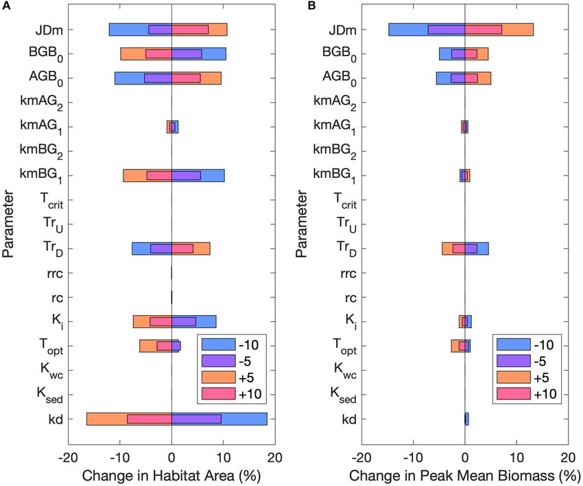
area at higher temperatures were likely caused by both decreased Sensitivity Analysis
primary production and increased respiration resulting in a Habitat area was most sensitive to changes in kd, kmBG1 , AGB0 ,
higher light compensation point and a shallower depth limit. BGB0 , and the date of mortality increase (JDm; Figure 7A).
Areal maps of habitat area under increasing SLR scenarios Changes to the half-saturation of light constant (Ki ) and the
show habitat area receding away from the deepening channels, downward translocation constant (TrD ) also influenced habitat
and being squeezed against the barrier islands and coastline area. Peak mean biomass in habitat areas was similarly most
(Figure 5). At +0.6 m SLR, over two thirds of the original habitat sensitive to changes in JDm, followed by AGB0 , BGB0 , and TrD
area was lost, most substantially in the southern third of BB-LEH (Figure 7B). Increasing either AGB0 or BGB0 resulted in a greater
(Figure 5C). At +0.8 m SLR, there was a near complete loss of peak mean biomass, but increasing BGB0 counter intuitively
seagrass in the north and south ends of the bay, with small beds resulted in a decline in habitat area (Figure 7). This dynamic
remaining near Barnegat Inlet (Figure 5D). By the maximum SLR was observed because when BGB0 was increased while AGB0
scenario, all suitable habitat disappeared (Figure 5E). remained constant, the proportion of BGB lost to mortality
and respiration exceeded the amount gained by downward
Seagrass Productivity translocation, resulting in fewer grid cells where BGB at some
While SLR had a drastic effect on seagrass habitat area, the point exceeded BGB0 . Habitat area and peak mean biomass were
effect of SLR on seagrass growth in areas that remained suitable both sensitive to changes in the January–June mortality rates
habitat was less severe (Figure 6A). Peak mean biomass in (kmAG1 and kmBG1 ) but were unaffected by changes to the
habitat areas decreased with increasing SLR scenarios, declining July–December mortality rates (kmAG2 and kmBG2 ). Modifying
approximately 20% from the base case with +0.8 m SLR the higher June-December mortality rates did not have an
(Figure 6A). Seagrass growth was highest at shallow depths, and effect, because habitat area and peak mean biomass were both
as depth increased with SLR, originally shallow areas that were determined by the first 45 days of growth (May 1 through June
still suitable habitat had increased light limitation and slower 15).
growth, thus lowering the mean biomass across habitat area. The optimal temperature for growth (Topt) influenced both
Temperature rise did not strongly affect seagrass productivity habitat area and peak mean biomass, where decreasing Topt
in areas with suitable habitat, shown by the minimal effect of resulted in a slight increase in both variables, with the opposite
temperature rise on seagrass growth rates or peak mean biomass effect occurring for increased Topt. The expansion of habitat
(Figure 6B). Temperature rise did increase the rate of seagrass with decreased Topt indicated that ambient water temperatures
die-off, likely due to higher losses due to respiration at higher during the important growing season (May–June) of the base
temperatures (Figure 6B). case were below the optimal temperature for growth, which helps
Integrated total biomass (tons C) across habitat area, which to explain the habitat expansion under low temperature rise
was a function of both suitable habitat area and seagrass growth, scenarios. Conversely, increasing Topt increased the difference
FIGURE 5 | Areal habitat maps showing increasing sea level rise scenarios (SLR) where (A) shows the base case scenario, (B) habitat after +0.3 m SLR, (C) habitat
after +0.6 m SLR, (D) habitat after +0.8 m SLR, and (E) habitat after +1.2 m SLR.
Frontiers in Marine Science | www.frontiersin.org 11 October 2020 | Volume 7 | Article 539946Scalpone et al. Seagrass Sensitivity to Future Climate FIGURE 6 | (A,B) Mean cumulative biomass (g C m−2 ) in habitat areas over time across (A) select sea level rise (SLR) scenarios, and (B) select temperature rise scenarios. (C,D) Total integrated biomass (tons C) across habitat areas for (C) select SLR scenarios, and (D) select temperature rise scenarios. between water temperatures and Topt which led to decreased (Supplementary Figure 4B), while the peak nutrient limitation habitat extent. The high temperature rise scenarios also increased factor (NLIM) was minimally affected by changes in Kwc or Ksed the difference between water temperatures and Topt, thereby (Supplementary Figure 4C). similarly resulting in decreased habitat area. Modifying the upward translocation coefficient (TU ), the critical temperature for germination (Tcrit ), the DIN half DISCUSSION saturation constants in the water column (Kwc ) or sediment (Ksed ), the root respiration rate at Topt (rc), or the root respiration We established a simple, spatially explicit seagrass model that coefficient (rrc) had little or no effect on habitat area or provided a theoretical setting to explore the effects of sea level peak mean biomass. and temperature rise on estuary-wide seagrass viability. Based on Primary productivity was strongly influenced by changes in the findings of other modeling studies, we hypothesized that SLR kd, moderately influenced by Ki and Topt, and not influenced would cause shifts in seagrass habitat distribution following the by Kwc or Ksed (Supplementary Figure 4A). The light limitation changes in light attenuation resulting from increased water depth factor (LLIM) was sensitive to change in both kd and Ki (Saunders et al., 2013; del Barrio et al., 2014; Davis et al., 2016). Frontiers in Marine Science | www.frontiersin.org 12 October 2020 | Volume 7 | Article 539946
Scalpone et al.                                                                                                                Seagrass Sensitivity to Future Climate

  FIGURE 7 | Percent change in (A) habitat area and (B) peak mean biomass from the base case for ±5 and ±10 of all parameters in sensitivity analysis. Legend unit
  is percent for all parameters expect JDm, which is in days. Refer to Table 2 for parameter definitions.

Previous studies suggested that temperature increases would                          Davis et al., 2016; 73.4%, del Barrio et al., 2014), and realized the
decrease seagrass growth by decreasing primary productivity                          observed biomass growth curves modeled in the source biomass
and increasing respiration rates (Carr et al., 2012; Jarvis et al.,                  production model (Straub et al., 2015). In model calibration,
2014), but the effects of temperature rise on both estuary-wide                      along with modifying mortality rate constants and initial biomass
productivity and habitat area had not previously been explored                       values, we increased the light-attenuation constant to 1.9 m−1 ,
in the literature. Our climate change simulations indicated that                     which was slightly above the median value observed (1.7 m−1 ,
SLR could lead to drastic decreases to suitable habitat extent in                    Ganju et al., 2014) to appropriately capture spatial placement
BB-LEH, squeezing seagrass beds landward toward the barrier                          along depth gradients. While the model did not predict seagrass
islands. Under the highest emissions scenario, projected SLR                         to the full observed depth range, the model predicted suitable
resulted in a complete loss of Z. marina in BB-LEH, exceeding                        habitat to 1.22 m which accounts for over 78% of mapped
the effects of SLR demonstrated for other systems (Saunders                          seagrass (Lathrop and Haag, 2011). Previous studies show that
et al., 2013; Davis et al., 2016). Contrary to our predictions,                      the accuracy of seagrass biomass models which rely on the inverse
temperature rise only slightly increased the rate of summer die-                     relationship to depth for habitat placement perform highest when
off and had a limited effect on habitat area, with substantial                       separate models are fit to areas with clear or turbid waters (Duarte
habitat loss observed only under the highest temperature rise                        et al., 2007). Within BB-LEH, high light attenuation results from
scenarios. Our results highlight the importance of creating site                     sediment-induced turbidity (Ganju et al., 2014), and increasing
specific predictions, as the species composition and regional                        the value of kd helped to reflect the potential impacts of variable
projections for climate change elevate the vulnerability of the                      turbidity across the bay.
seagrass meadows in BB-LEH to losses due to SLR.                                         Much of the deviation between the modeled and observed
                                                                                     habitat extent occurred from the model overestimating habitat
Model Performance                                                                    presence in locations where it was not actually observed, most
The calibrated model achieved high spatial accuracy in the base                      distinctly surrounding the two inlets, Barnegat Inlet and Little
case, comparable to other similar modeling studies (55.1–91.5%,                      Egg Harbor Inlet. While these areas are shallow enough to

Frontiers in Marine Science | www.frontiersin.org                               13                                         October 2020 | Volume 7 | Article 539946
Scalpone et al. Seagrass Sensitivity to Future Climate
support seagrass communities, the rapid geomorphic change and SLR (Miselis et al., 2016). Even if the surrounding salt marshes
high tidal velocities near the inlets could prevent seagrass from were eroded in the future, there is no guarantee that seagrass
colonizing the shoals in these regions (Stevens and Lacy, 2012). would be able to colonize the new territory, as eroded marsh
Accounting for geomorphic change or current velocity in the sediments do not serve as adequate substrate for Z. marina seeds
model could help improve habitat prediction accuracy (Valle (Wicks et al., 2009). Alternatively, if we were to assume that SLR
et al., 2014). Including these dynamics in future work would would breach the barrier islands without converting to natural
require additional parameterization of the biomass production habitat, increased connectivity with the Atlantic Ocean would
model to establish the physiological response of seagrass growth introduce a suite of hydrodynamic changes that have been shown
to changes in these hydrodynamic variables (Peralta et al., 2006). to significantly impact seagrass habitat, such as increased wave
Alternatively, the areas surrounding the inlets could experience exposure, tidal range, and current velocity (Tanaka and Nakaoka,
higher light attenuation due to resuspension-induced turbidity 2004; del Barrio et al., 2014; Saunders et al., 2014; Valle et al., 2014;
which was not explicitly modeled in this analysis. Implementing Defne and Ganju, 2015). Decreased wave sheltering from coral
spatially variable light-attenuation constants that account for reefs due to SLR resulted in decreased seagrass habitat availability
turbidity could improve our model predictions (Duarte et al., in a tropical coastal system (Saunders et al., 2014), which is a
2007), particularly because habitat suitability was highly sensitive protection currently supplied by the barrier islands in BB-LEH
to changes in kd. (Defne and Ganju, 2015). Increased tidal range would subject a
greater area of seagrass habitat to emergence stress, which also
negatively impacts seagrass growth (Tanaka and Nakaoka, 2004;
Seagrass Response to Climate Change Kim et al., 2013). While these scenarios are possible, the current
Scenarios state of coastline hardening and frequent dredging to maintain
Increasing sea level resulted in a consistent decline in habitat current navigable waterways in BB-LEH indicate that it would
area, demonstrating the sensitivity of Z. marina distribution to be highly optimistic to model a future scenario that assumes
changes in depth. Our model projected that as sea level increased, urban and marsh land will convert to open water unimpeded by
currently available habitat shifted closer to the barrier islands, anthropogenic intervention (Kennish, 2001; Miselis et al., 2016).
following the shifting light attenuation gradient. Under the While the landward migration of suitable habitat with SLR was
assumption that SLR will not change the boundaries of available in line with the findings of similar modeling work, the magnitude
habitat, seagrass habitat was pushed to the estuary boundaries of habitat loss due to SLR exceeded what other studies have
and prevented from establishing new habitat. Saunders et al. suggested for estuaries in other regions. Our model simulated
(2013) termed this process as “coastal squeeze,” a pattern that that 100% of suitable habitat disappeared under the maximum
has been well-documented in other modeling studies which SLR scenario. In contrast, Davis et al. (2016) found a maximum
do not allow for habitat expansion under SLR (Davis et al., seagrass habitat loss of 44%, and Saunders et al. (2013) reported
2016; Mills et al., 2016). Other studies that have modeled the a 17% loss in seagrass habitat, under their respective maximum
effects of increasing light limitation on seagrass habitat have SLR scenarios. One reason for this disparity comes from the
similarly shown that available habitat is primarily determined value used for maximum SLR. Our maximum SLR scenario
by light climate. Saunders et al. (2017) simulated that increasing (+1.2 m) exceeded the scenario used in Davis et al. (+0.75 m;
suspended sediment load decreased seagrass habitat availability 2016), because we used the projected rise for the Eastern North
by increasing light attenuation. Likewise, Cerco and Moore American coast, whereas Davis et al. (2016) used the global
(2001) explored the effects of eutrophication on seagrass average projection. Saunders et al. (2013) used a comparable
distribution and growth, and found that seagrass density spatially magnitude of SLR (+1.1 m), but their study system supported
followed the same contours as light attenuation, with decreasing six seagrass species, two of which had greater depth limits than
density as light attenuation increased. Z. marina (Duarte, 1991). The disparity between our results
The modeled habitat loss due to coastal squeeze under SLR underscores the need for site specific predictions, as the low
was partially due to constraining the model domain to the current species diversity and heightened risk of sea level rise along the
boundaries based on the highly developed coastline (Lathrop Atlantic coast elevate the vulnerability of the seagrass meadows
and Bognar, 2001) and slow erosion rates of surrounding salt in BB-LEH to losses due to climate change.
marshes (Leonardi et al., 2016). Other studies have demonstrated The effects of sea level rise far outweighed the effects of
that if coastal areas are allowed to naturally convert to open temperature rise on seagrass growth and habitat extent for
water under SLR, marine habitats have the potential to expand modeled meadows in BB-LEH. Habitat area slightly expanded for
in the future (Valle et al., 2014; Mills et al., 2016; Schuerch low temperature rise scenarios and decreased substantially only
et al., 2018). Furthermore, in a coastal system without human at the highest temperature rise scenarios. Increasing temperature
modification, SLR would cause the barrier islands to shift had little effect on peak mean biomass and only slightly increased
landward, pushing shallow shoals into previously deep water the rate of seagrass loss during summer and fall months.
and allowing seagrass communities to maintain suitable habitat Temperature has been shown to influence seagrass depth limits
area (Saunders et al., 2013). However, analysis of barrier island through the trade-off between respiration rates and primary
rollover in BB-LEH following Hurricane Sandy demonstrated productivity in low light environments (Lee et al., 2007; Tanaka
that the highly managed, highly developed barrier islands will and Nakaoka, 2007). The sensitivity of habitat area to changes
likely not be able to shift to sustain available habitat under in Topt indicated that the leading contributor to habitat loss at
Frontiers in Marine Science | www.frontiersin.org 14 October 2020 | Volume 7 | Article 539946Scalpone et al. Seagrass Sensitivity to Future Climate
high temperatures in our model was likely decreased primary the end of the year to simulate increased mortality in summer
productivity rather than increased respiration. and leaf sloughing in fall and winter. Using constant mortality
Other studies have demonstrated non-linear interactions rates could have oversimplified the impacts of temperature,
between temperature and sea level. For example, in Chesapeake leading to the low biomass responses to changes in temperature.
Bay, seagrass habitat in shallow regions where light was Furthermore, the most severe impacts of increased temperatures
not limiting was found to be more vulnerable to extreme on seagrass have been demonstrated to occur during marine heat
temperatures (Lefcheck et al., 2017). While seagrass meadows in waves (Moore and Jarvis, 2008; Moore et al., 2012; Smale and
shallow areas did experience higher temperature increases in our Wernberg, 2013), which are expected to increase in frequency and
model, reflecting this dynamic, we did not simulate an increased duration with increased global temperatures (Oliver et al., 2018).
influence of temperature when seagrass habitat was limited to Our temperature scenarios represented increases in mean air
shallow regions under increasing sea level scenarios. The effects temperature expected with climate change, and did not simulate
of temperature rise on habitat area remained constant with increased variability in temperature extremes.
SLR, indicating that high temperature increases could further Based on the sensitivity analysis, mortality parameters, such
exacerbate the negative impacts of SLR on habitat area. as the date on which high summer-fall mortality was triggered
While light climate is often found to be the most influential in the model and the January–June mortality rates, were highly
factor affecting seagrass growth (Lee et al., 2007), both influential on model results, highlighting the importance of
experimental and modeling studies support the hypothesis accurately parameterizing mortality. Habitat area and peak mean
that temperature rise will lower seagrass growth and increase biomass were only sensitive to parameters that impact the first
mortality (Marsh et al., 1986; Carr et al., 2012; Repolho et al., 45 days of growth, i.e., the time period before high mortality
2017). Jarvis et al. (2014) assessed the response of simulated was triggered. Previous studies have demonstrated that seagrass
seagrass growth to multiple years of temperature stress, and population viability relies on successful spring-time growth
found that with only a 1◦ C increase in temperature for 1 year, (Moore et al., 1997), which aligns with our model’s reliance
seagrass were unable to recover. Other studies have shown a on late spring growth to define successful habitat. While the
similar reduction of productivity due to temperature rise, with date of mortality increase was determined to match present-
dramatic losses of biomass occurring when summer temperatures day conditions, increases to year-round temperatures could shift
exceed 30◦ C (Davis et al., 2016). Using an SDM for Z. marina summer mortality to earlier in the year, which was not reflected
populations along the Atlantic Coast of North America, Wilson in our temperature rise scenarios (Clausen et al., 2014).
and Lotze (2019) projected a complete extinction of seagrass in
BB-LEH with a temperature increase projected under the IPCC’s Model Limitations and Caveats
maximum emissions scenario. However, their model assumed An important goal of this study was to provide a simple system
that water temperatures were already limiting in BB-LEH. Straub approach to efficiently test the sensitivity of seagrass to changes
et al. (2015) have shown that daily mean water temperatures in in sea level and temperature, and thus we did not aim to capture
BB-LEH seagrass meadows ranged between 0 and 28◦ C with the every biogeochemical and hydrodynamic process that impacts
highest temperatures not lasting more than 5 consecutive days, seagrass meadows. However, the exclusion of other processes
shorter than the time periods observed to result in Z. marina limits the extent to which our model can fully capture responses
thermal die-off events (Moore and Jarvis, 2008). Therefore, while to future changes in physical conditions. One such limitation
temperature rise is a demonstrated threat to Z. marina, our was the exclusion of epiphytes and phytoplankton, which can
model results suggest that rising sea level presents a more severe be important controls on light climate, and respond to changes
threat to BB-LEH. Under our conservative SLR scenario, which in temperature and nutrient availability (Cerco and Moore,
increased sea level by less than half of the projected increases 2001; Thomsen et al., 2012; del Barrio et al., 2014). Because we
under a maximum emissions scenario, habitat area dropped by isolated the impacts of water depth and temperature on seagrass,
over 40%, and integrated total biomass fell by nearly half. The and did not modify nutrients, we did not simulate changes
Wilson and Lotze (2019) study did not investigate SLR and the in nutrient-sensitive epiphytes and phytoplankton. Their effects
associated changes to light availability. were, however, included in the model implicitly, as epiphytes
The muted response of habitat area and biomass production and phytoplankton factor into present day habitat distribution
to increasing temperature in our model compared to the impacts and growth for which the model was calibrated. Furthermore,
demonstrated in other studies could be due to insufficient the empirical evaluation of kd in BB-LEH by Ganju et al. (2014)
representation of mortality temperature dependence in the included the effects of phytoplankton on light attenuation. If
biomass production model, and the lack of extreme temperature epiphytes and phytoplankton were to be modeled explicitly, more
events in our climate scenarios. Although extreme temperatures sophisticated nutrient dynamics would need to be employed in
have been repeatedly linked to spikes in mortality (Moore and the model to capture spatial patterns in eutrophication (del Barrio
Jarvis, 2008; Smale and Wernberg, 2013), the mathematical et al., 2014; Ganju et al., 2014).
relationship between mortality and temperature is not well- Because the hydrodynamic model was not re-run under the
established for seagrass in BB-LEH and was therefore not climate change scenarios, we did not simulate any bathymetric
explicitly included in the Straub et al. (2015) model. This was changes that could occur due to increased erosion and accretion
partly compensated in the model by employing two constant under SLR. While shoal accretion could contribute to seagrass
mortality rates, with higher mortality from mid-June through habitat redistribution or expansion (Barillé et al., 2010), changes
Frontiers in Marine Science | www.frontiersin.org 15 October 2020 | Volume 7 | Article 539946You can also read