An oscillating computational model can track pseudo-rhythmic speech by using linguistic predictions
←
→
Page content transcription
If your browser does not render page correctly, please read the page content below
RESEARCH ARTICLE

                                      An oscillating computational model can
                                      track pseudo-rhythmic speech by using
                                      linguistic predictions
                                      Sanne ten Oever1,2,3*, Andrea E Martin1,2
                                      1
                                       Language and Computation in Neural Systems group, Max Planck Institute for
                                      Psycholinguistics, Nijmegen, Netherlands; 2Donders Centre for Cognitive
                                      Neuroimaging, Radboud University, Nijmegen, Netherlands; 3Department of
                                      Cognitive Neuroscience, Faculty of Psychology and Neuroscience, Maastricht
                                      University, Maastricht, Netherlands

                                      Abstract Neuronal oscillations putatively track speech in order to optimize sensory processing.
                                      However, it is unclear how isochronous brain oscillations can track pseudo-rhythmic speech input.
                                      Here we propose that oscillations can track pseudo-rhythmic speech when considering that speech
                                      time is dependent on content-based predictions flowing from internal language models. We show
                                      that temporal dynamics of speech are dependent on the predictability of words in a sentence. A
                                      computational model including oscillations, feedback, and inhibition is able to track pseudo-
                                      rhythmic speech input. As the model processes, it generates temporal phase codes, which are a
                                      candidate mechanism for carrying information forward in time. The model is optimally sensitive to
                                      the natural temporal speech dynamics and can explain empirical data on temporal speech illusions.
                                      Our results suggest that speech tracking does not have to rely only on the acoustics but could also
                                      exploit ongoing interactions between oscillations and constraints flowing from internal language
                                      models.

*For correspondence:
sanne.tenoever@mpi.nl
                                      Introduction
Competing interests: The              Speech is a biological signal that is characterized by a plethora of temporal information. The tempo-
authors declare that no
                                      ral relationship between subsequent speech units allows for the online tracking of speech in order to
competing interests exist.
                                      optimize processing at relevant moments in time (Jones and Boltz, 1989; Large and Jones, 1999;
Funding: See page 21                  Giraud and Poeppel, 2012; Ghitza and Greenberg, 2009; Ding et al., 2017; Arvaniti, 2009; Poep-
Preprinted: 07 December 2020          pel, 2003). Neural oscillations are a putative index of such tracking (Giraud and Poeppel, 2012;
Received: 03 March 2021               Schroeder and Lakatos, 2009). The existing evidence for neural tracking of the speech envelope is
Accepted: 16 July 2021                consistent with such a functional interpretation (Luo et al., 2013; Keitel et al., 2018). In these
Published: 02 August 2021             accounts, the most excitable optimal phase of an oscillation is aligned with the most informative
                                      time point within a rhythmic input stream (Schroeder and Lakatos, 2009; Lakatos et al., 2008;
Reviewing editor: Anne Kösem,
Lyon Neuroscience Research
                                      Henry and Obleser, 2012; Herrmann et al., 2013; Obleser and Kayser, 2019). However, the range
Center, France                        of onset time difference between speech units seems more variable than fixed oscillations can
                                      account for (Rimmele et al., 2018; Nolan and Jeon, 2014; Jadoul et al., 2016). As such, it remains
   Copyright ten Oever and
                                      an open question how is it possible that oscillations can track a signal that is at best only pseudo-
Martin. This article is distributed
                                      rhythmic (Nolan and Jeon, 2014).
under the terms of the Creative
Commons Attribution License,              Oscillatory accounts tend to focus on the prediction in the sense of predicting ‘when’, rather than
which permits unrestricted use        predicting ‘what’: oscillations function to align the optimal moment of processing given that timing
and redistribution provided that      is predictable in a rhythmic input structure. If rhythmicity in the input stream is violated, oscillations
the original author and source are    must be modulated to retain optimal alignment to incoming information. This can be achieved
credited.                             through phase resets (Rimmele et al., 2018; Meyer, 2018), direct coupling of the acoustics to

ten Oever and Martin. eLife 2021;10:e68066. DOI: https://doi.org/10.7554/eLife.68066                                                     1 of 25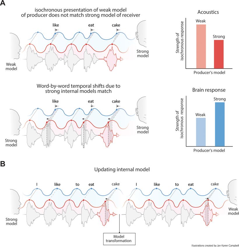
Research article                                                                                                    Neuroscience

                                   oscillations (Poeppel and Assaneo, 2020), or the use of many oscillators at different frequencies
                                   (Large and Jones, 1999). However, the optimal or effective time of processing stimulus input might
                                   not only depend on when you predict something to occur, but also depend on what stimulus is actu-
                                   ally being processed (Ten Oever et al., 2013; Martin, 2016; Rosen, 1992; deen et al., 2017).
                                       What and when are not independent, and certainly not from the brain’s-eye-view. If continuous
                                   input arrives to a node in an oscillatory network, the exact phase at which this node reaches thresh-
                                   old activation does not only depend on the strength of the input, but also depend on how sensitive
                                   this node was to start with. Sensitivity of a node in a language network (or any neural network) is nat-
                                   urally affected by predictions in the what domain generated by an internal language model (Mar-
                                   tin, 2020; Marslen-Wilson, 1987; Lau et al., 2008; Nieuwland, 2019). We define internal language
                                   model as the individually acquired statistical and structural knowledge of language stored in the
                                   brain. A virtue of such an internal language model is that it can predict the most likely future input
                                   based on the currently presented speech information. If a language model creates strong predic-
                                   tions, we call it a strong model. In contrast, a weak model creates no or little predictions about
                                   future input (note that the strength of individual predictions depends not only on the capability of
                                   the system to create a prediction, but also on the available information). If a node represents a
                                   speech unit that is likely to be spoken next, a strong internal language model will sensitize this node
                                   and it will therefore be active earlier, that is, on a less excitable phase of the oscillation. In the
                                   domain of working memory, this type of phase precession has been shown in rat hippocampus
                                   (O’Keefe and Recce, 1993; Malhotra et al., 2012) and more recently in human electroencephalog-
                                   raphy (Bahramisharif et al., 2018). In speech, phase of activation and perceived content are also
                                   associated (Ten Oever and Sack, 2015; Kayser et al., 2016; Di Liberto et al., 2015; Ten Oever
                                   et al., 2016; Thézé et al., 2020), and phase has been implicated in tracking of higher-level linguistic
                                   structure (Meyer, 2018; Brennan and Martin, 2020; Kaufeld et al., 2020a). However, the direct
                                   link between phase and the predictability flowing from a language model has yet to be established.
                                       The time of speaking/speed of processing is not only a consequence of how predictable a speech
                                   unit is within a stream, but also a cue for the interpretation of this unit. For example, phoneme cate-
                                   gorization depends on timing (e.g., voice onsets, difference between voiced and unvoiced pho-
                                   nemes), and there are timing constraints on syllable durations (e.g., the theta syllable Poeppel and
                                   Assaneo, 2020; Ghitza, 2013) that affect intelligibility (Ghitza, 2012). Even the delay between
                                   mouth movements and speech audio can influence syllabic categorizations (Ten Oever et al., 2013).
                                   Most oscillatory models use oscillations for parsing, but not as a temporal code for content
                                   (Panzeri et al., 2015; Kayser et al., 2009; Mehta et al., 2002; Lisman and Jensen, 2013). How-
                                   ever, the time or phase of presentation does influence content perception. This is evident from two
                                   temporal speech phenomena. In the first phenomena, the interpretation of an ambiguous short /a/
                                   or long vowel /a:/ depends on speech rate (in Dutch; Reinisch and Sjerps, 2013; Kösem et al.,
                                   2018; Bosker and Reinisch, 2015). Specifically, when speech rates are fast the stimulus is inter-
                                   preted as a long vowel and vice versa for slow rates. However, modulating the entrainment rate
                                   effectively changes the phase at which the target stimulus – which is presented at a constant speech
                                   rate – arrives (but this could not be confirmed in Bosker and Kösem, 2017). A second speech phe-
                                   nomena shows the direct phase-dependency of content (Ten Oever and Sack, 2015; Ten Oever
                                   et al., 2016). Ambiguous /da/-/ga/ stimuli will be interpreted as a /da/ on one phase and a /ga/ on
                                   another phase. This was confirmed in both a EEG and a behavioral study. An oscillatory theory of
                                   speech tracking should account for how temporal properties in the input stream can alter what is
                                   perceived.
                                       In the speech production literature, there is strong evidence that the onset times (as well as dura-
                                   tion) of an uttered word is modulated by the frequency of that word in the language (O’Malley and
                                   Besner, 2008; Monsell, 1991; Monsell et al., 1989; Powers, 1998; Piantadosi, 2014) showing that
                                   internal language models modulate the access to or sensitivity of a word node (Martin, 2020;
                                   Hagoort, 2017). This word-frequency effect relates to the access to a single word. However, it is
                                   likely that during ongoing speech internal language models use the full context to estimate upcom-
                                   ing words (Beattie and Butterworth, 1979; Pluymaekers et al., 2005a; Lehiste, 1972). If so, the
                                   predictability of a word in context should provide additional modulations on speech time. Therefore,
                                   we predict that words with a high predictability in the producer’s language model should be uttered
                                   relatively early. In this way, word-to-word onset times map to the predictability level of that word
                                   within the internal model. Thus, not only the processing time depends on the predictability of a

ten Oever and Martin. eLife 2021;10:e68066. DOI: https://doi.org/10.7554/eLife.68066                                                 2 of 25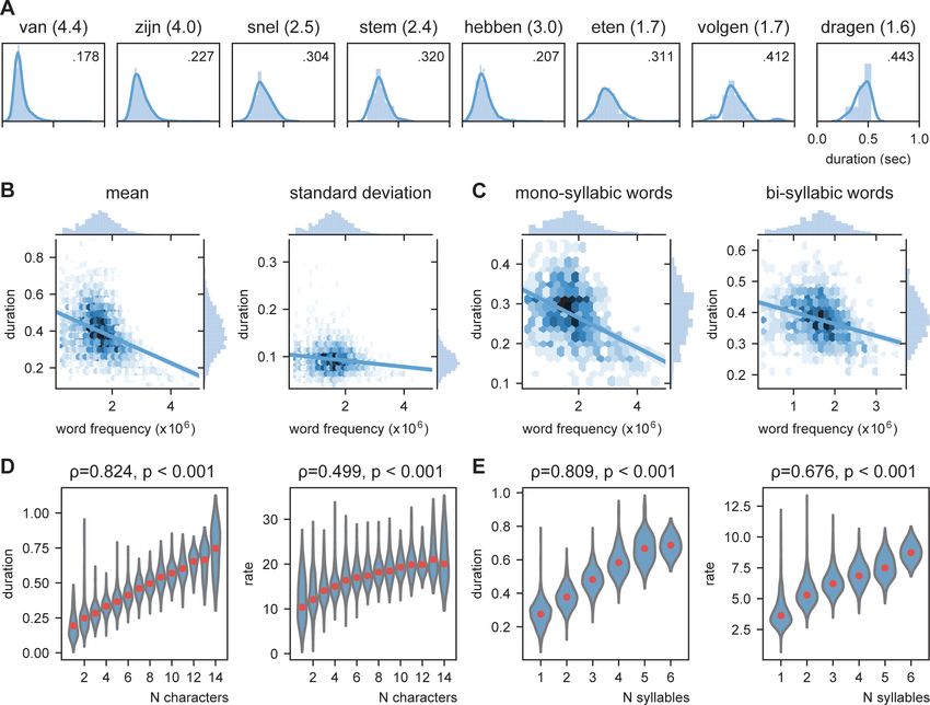
Research article                                                                                                    Neuroscience

                                   word (faster processing for predictable words; see Gwilliams et al., 2020; Deacon et al., 1995, and
                                   Aubanel and Schwartz, 2020 showing that speech time in noise matters), but also the production
                                   time (earlier uttering of predicted words).
                                       Language comprehension involves the mapping of speech units from a producer’s internal model
                                   to the speech units of the receiver’s internal model. In other words, one will only understand what
                                   someone else is writing or saying if one’s language model is sufficiently similar to the speakers (and
                                   if we speak in Dutch, fewer people will understand us). If the producer’s and receiver’s internal lan-
                                   guage model have roughly matching top-down constrains, they should similarly influence the speed
                                   of processing (either in production or perception; Figure 1A–C). Therefore, if predictable words
                                   arrive earlier (due to high predictability in the producer’s internal model), the receiver also expects
                                   the content of this word to match one of the more predictable ones from their own internal model
                                   (Figure 1C). Thus, the phase of arrival depends on the internal model of the producer and the
                                   expected phase of arrival depends on the internal model of the receiver (Figure 1D). If this is true,
                                   pseudo-rhythmicity is fully natural to the brain, and it provides a means to use time or arrival phase
                                   as a content indicator. It also allows the receiver to be sensitive to less predictable words when they
                                   arrive relatively late. Current oscillatory models of speech parsing do not integrate the constraints
                                   flowing from an internal linguistic model into the temporal structure of the brain response. It is
                                   therefore an open question whether the oscillatory model the brain employs is actually attuned to
                                   the temporal variations in natural speech.
                                       Here, we propose that neural oscillations can track pseudo-rhythmic speech by taking into
                                   account that speech timing is a function of linguistic constrains. As such we need to demonstrate
                                   that speech statistics are influenced by linguistic constrains as well as showing how oscillations can
                                   be sensitive to this property in speech. We approach this hypothesis as follows: First, we demon-
                                   strate that in natural speech timing depends on linguistics predictions (temporal speech properties).
                                   Then, we model how oscillations can be sensitive to these linguistic predictions (modeling speech
                                   tracking). Finally, we validate that this model is optimally sensitive to the natural temporal properties
                                   in speech and displays temporal speech illusions (model validation). Our results reveal that tracking
                                   of speech needs to be viewed as an interaction between ongoing oscillations as well as constraints
                                   flowing from an internal language model (Martin, 2016; Martin, 2020). In this way, oscillations do
                                   not have to shift their phase after every speech unit and can remain at a relatively stable frequency
                                   as long as the internal model of the speaker matches the internal model of the perceiver.

                                   Results
                                   Temporal speech properties
                                   Word frequency influences word duration
                                   To extract the temporal properties in naturally spoken speech we used the Corpus Gesproken
                                   Nederlands (CGN; [Version 2.0.3; 2014]). This corpus consists of elaborated annotations of over 900
                                   hr of spoken Dutch and Flemish words. We focus here on the subset of the data of which onset and
                                   offset timings were manually annotated at the word level in Dutch. Cleaning of the data included
                                   removing all dashes and backslashes. Only words were included that were part of a Dutch word2vec
                                   embedding (github.com/coosto/dutch-word-embeddings; Nieuwenhuijse, 2018; needed for later
                                   modeling) and required to have a frequency of at least 10 in the corpus. All other words were
                                   replaced with an  label. This resulted in 574,726 annotated words with 3096 unique
                                   words. Two thousand and forty-eight of the words were recognized in the Dutch Wordforms data-
                                   base in CELEX (Version 3.1) in order to extract the word frequency as well as the number of syllables
                                   per word (later needed to fit a regression model). Mean word duration was 0.392 s, with an average
                                   standard deviation of 0.094 s (Figure 2—figure supplement 1). By splitting up the data in sequen-
                                   ces of 10 sequential words, we could extract the average word, syllable, and character rate (Fig-
                                   ure 2—figure supplements 2 and 3). The reported rates fall within the generally reported ranges
                                   for syllables (5.2 Hz) and words (3.7 Hz; Ding et al., 2017; Pellegrino and Coupé, 2011).
                                      We predict that knowledge about the language statistics influences the duration of speech units.
                                   As such we predict that more prevalent words will have on average a shorter duration (also reported
                                   in Monsell et al., 1989). In Figure 2A, the duration of several mono- and bi-syllabic words are listed
                                   with their word frequency. From these examples, it seems that words with higher word frequency

ten Oever and Martin. eLife 2021;10:e68066. DOI: https://doi.org/10.7554/eLife.68066                                                 3 of 25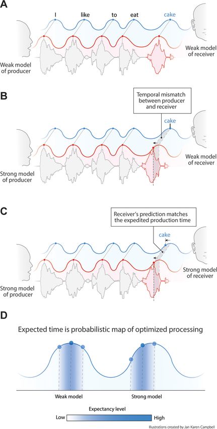
Research article                                                                                                             Neuroscience

                                   Figure 1. Proposed interaction between speech timing and internal linguistic models. (A) Isochronous production
                                   and expectation when there is a weak internal model (even distribution of node activation). All speech units arrive
                                   around the most excitable phase. (B) When the internal model of the producer does not align with the model of
                                   the receiver temporal alignment and optimal communication fails. (C) When both producer and receiver have a
                                   strong internal model, speech is non-isochronous and not aligned to the most excitable phase, but fully expected
                                   by the brain. (D) Expected time is a constraint distribution in which the center can be shifted due to linguistic
                                   constraints.

ten Oever and Martin. eLife 2021;10:e68066. DOI: https://doi.org/10.7554/eLife.68066                                                           4 of 25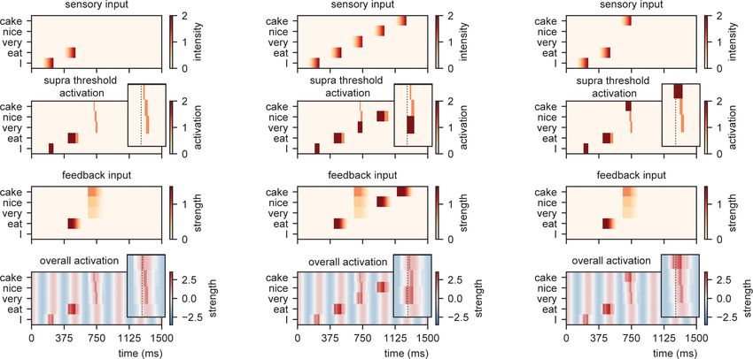
Research article                                                                                                             Neuroscience

Figure 2. Word frequency modulates word duration. (A) Example of mono- and bi-syllabic words of different word frequencies in brackets (van=from,
zijn=be, snel=fast, stem=voice, hebben=have, eten=eating, volgend=next, toekomst=future). Text in the graph indicates the mean word duration. (B)
Relationship between word frequency and duration. Darker colors mean more values. (C) same as (B) but separately for mono- and bi-syllabic words. (D)
Relationship character amount and word duration. The longer the words, the longer the duration (left). The increase in word duration does not follow a
fixed number per character as duration as measured by rate increases. (E) same as (D) but for number of syllables. Red dots indicate the mean.
The online version of this article includes the following figure supplement(s) for figure 2:
Figure supplement 1. Distribution of mean duration (A) and of average rate (B).
Figure supplement 2. Distribution of mean duration split up for word length (in characters).
Figure supplement 3. Distribution of mean duration split up for syllable length.

                                     generally have a shorter duration. To test this statistically we entered word frequency in an ordinary
                                     least square regression with number of syllables as control. Both number of syllables (coefficient =
                                     0.1008, t(2843) = 75.47, p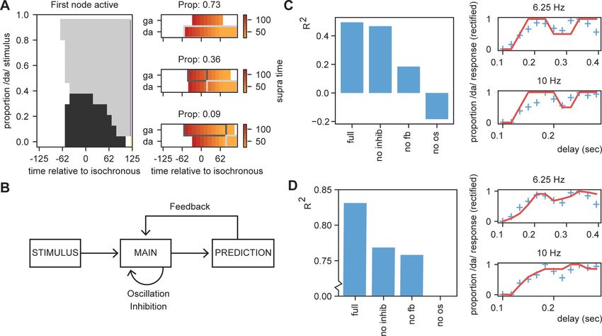
Research article                                                                                                    Neuroscience

                                   (number of characters 0.824, p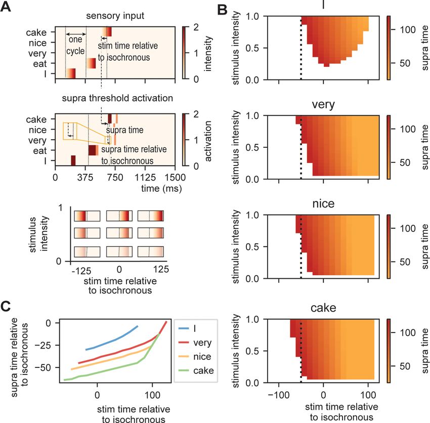
Research article                                                                                                                Neuroscience

Figure 3. RNN output influence word onset differences. (A) Sequences of 10 words were entered in an RNN in order to predict the content of the next
word. Three examples are provided of input data with the label (bold word) and probability output for three different words. The regression model
showed a relation between the duration of last word in the sequence and the predictability of the next word such that words were systematically
shorter when the next word was more predictable according to the RNN output (illustrated here with the shorted black boxes). (B) Regression line
estimated at mean value of word duration and bigram. (C) Scatterplot of prediction and onset difference of data within ± 0.5 standard deviation of
word duration and bigram. Note that for (B) and (C), the axes are linear on the transformed values. (D) Regression line for the correlation between
logarithm of variance of the prediction and theta power. (E) None-transformed distribution of variance of the predictions (within a sentence). Translation
of the sentences in (A) from top to bottom: ‘... that it has for me and while you have no answer [on]’, ‘... the only real hope for us humans is a firm and
[sure]’, ‘... a couple of glass doors in front and then it would not have been [in]’.
The online version of this article includes the following figure supplement(s) for figure 3:
Figure supplement 1. Recurrent neural network evaluation.
Figure supplement 2. RNN prediction distributions.

                                              All predictors except word frequency of the previous word showed a significant effect (Table 1).
                                          The variance explained by word frequency was likely captured by the mean duration variable of the
                                          previous word, which is correlated to word frequency. The RNN predictor could capture more vari-
                                          ance than the bigram model, suggesting that word duration is modulated by the level of predictabil-
                                          ity within a fuller context than just the conditional probability of the current word given the previous

Table 1. Summary of regression model for logarithm of onset difference of words.
Variable                           Trans               B                 b                   SE                t                    p                  VIF
Intercept                          x                   0.9719                                0.049             19.764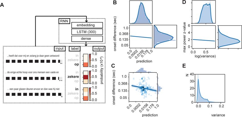
Research article                                                                                                          Neuroscience

                                   word (Figure 3B,C). Importantly, it was necessary to use the trained RNN model as a predictor;
                                   entering the RNN predictions after the first training cycle (of a total of 100) did not results in a signif-
                                   icant predictor (t(4837) = 1.191, p=0.234). Also adding the predictor word frequency of the current
                                   word did not add significant information to the model (F(1, 4830) = 0.2048, p=0.651). These results
                                   suggest that words are systematically lengthened (or pauses are added. However, the same predic-
                                   tors are also significant when excluding sentences containing pauses) when the next word is not
                                   strongly predicted by the internal model. We also investigate whether RNN predictions have an
                                   influence on the duration of the word that has to be uttered. We found no effect on the duration
                                   (Supporting Table 1).

                                   Sentence isochrony depends on prediction variance
                                   In the previous section, we investigated word-to-word onsets, but did not investigate how this influ-
                                   ences the temporal properties within a full sentence. In a regular sentence, predictability values
                                   change from word-to-word. Based on the previous results, it is expected that overall sentences with
                                   a more stable predictability level (sequential words are equally predictable) should be more isochro-
                                   nous than sentences in which the predictability shifts from high to low. This prediction is based on
                                   the observation that when predictions are equal the expected shift is the same, while for varying pre-
                                   dictions, temporal shifts vary (Figure 3B,C).
                                       To test this hypothesis, we extracted the RNN prediction for 10 subsequent words. Then we
                                   extracted the variance of the prediction across those 10 words and extracted the word onset itself.
                                   We created a time course at which word onset were set to 1 (at a sampling rate of 100 Hz). Then we
                                   performed an fast Fourier transform (FFT) and extracted z-transformed power values over a 0–15 Hz
                                   interval. The power at the maximum power value with the theta range (3–8 Hz) was extracted. These
                                   max z-scores were correlated with the log transform of the variance (to normalize the skewed vari-
                                   ance distribution; Figure 3E). We found a weak, but significant negative correlation (r = 0.062,
                                   p
                                                                               <      3  BaseInhib; Ta
                                                                    inhibðTaÞ ¼ 3  BaseInhib; 20  Ta
                                                                                     BaseInhib; Ta>100
                                                                               :

                                   in which BaseInhib is a constant for the base level of inhibition (negative value, set to 0.2). As such
                                   nodes are by default inhibited, as soon as they get activated above threshold (activation threshold
                                   set at 1) Ta sets to zero. Then, the node will have suprathreshold activation, which after 20 ms
                                   returns to increased inhibition until the base level of inhibition is returned. These values are set to

ten Oever and Martin. eLife 2021;10:e68066. DOI: https://doi.org/10.7554/eLife.68066                                                      8 of 25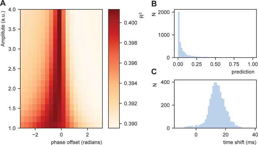
Research article                                                                                                      Neuroscience

                                   reflect early excitation and longer lasting inhibition, which are only loosely related to neurophysio-
                                   logical time scales. The oscillation is a constant oscillator:

                                                                               oscðT Þ ¼ Am  e2pi!Tþi’                                      (3)

                                   in which Am is the amplitude of the oscillator, w the frequency, and j the phase offset. As such we
                                   assume a stable oscillator which is already aligned to the average speech rate (see Rimmele et al.,
                                   2018; Poeppel and Assaneo, 2020 for phase alignment models). The model used for the current
                                   simulation has one an input layer (l 1 level) and one single layer of semantic word nodes (l level)
                                   that receives feedback from a higher level layer (l+1 level). As such only the word (l) level is modeled
                                   according to Equation 1–3 and the other levels form fixed input and feedback connection patterns.
                                   Even though the feedback influences the activity at the word level, it does not cause a phase reset
                                   as the phase of the oscillation does not change in response to this feedback.

                                   Language models influence time of activation
                                   To illustrate how STiMCON can explain how processing time depends on the prediction of internal
                                   language models, we instantiated a language model that had only seen three sentences and five
                                   words presented at different probabilities (I eat cake at 0.5 probability, I eat nice cake at 0.3 proba-
                                   bility, I eat very nice cake at 0.2 probability; Table 2). While in the brain the prediction should add
                                   up to 1, we can assume that the probability is spread across a big number of word nodes of the full
                                   language model and therefore neglectable. This language model will serve as the feedback arriving
                                   from the l+1-level to the l-level. The l-level consists of five nodes that each represent one of the
                                   words and receives proportional feedback from l+1 according to Table 2 with a delay of 0.9*w sec-
                                   onds, which then decays at 0.01 unit per millisecond and influences the l-level at a proportion of 1.5.
                                   The 0.9*w was defined as we hypothesized that onset time would be loosely predicted around on
                                   oscillatory cycle, but to be prepared for input slightly earlier (which of course happens for predict-
                                   able stimuli), we set it to 0.9 times the length of the cycle. The decay is needed and set such that
                                   the feedback would continue around a full theta cycle. The proportion was set empirically such to
                                   ensure that strong feedback did cause suprathreshold activation at the active node. The feedback is
                                   only initiated when supra-activation arrives due to l 1-level bottom-up input. Each word at the l 1-
                                   level input is modeled as a linearly function to the individual nodes lasting length of 125 ms (half a
                                   cycle, ranging from 0 to 1 arbitrary units). As such, the input is not the acoustic input itself but rather
                                   reflects a linear increase representing the increasing confidence of a word representing the specific
                                   node. j is set such that the peak of a 4 Hz oscillation aligns to the peak of sensory input of the first
                                   word. Sensory input is presented at a base stimulus onset asynchrony of 250 ms (i.e., 4 Hz).
                                       When we present this model with different sensory inputs at an isochronous rhythm of 4 Hz, it is
                                   evident that the timing at which different nodes reach activation depends on the level of feedback
                                   that is provided (Figure 4). For example, while the /I/-node needs a while to get activated after the
                                   initial sensory input, the /eat/-node is activated earlier as it is pre-activated due to feedback. After
                                   presenting /eat/, the feedback arrives at three different nodes and the activation timing depends on
                                   the stimulus that is presented (earlier activation for /cake/ compared to /very/).

                                   Table 2. Example of a language model.
                                   This model has seen three sentences at different probabilities. Rows represent the prediction for the
                                   next word, e.g., /I/ predicts /eat/ at a probability of 1, but after /eat/ there is a wider distribution.
                                                        I                  Eat                   Very              Nice                  Cake
                                   I                    0                  1                     0                 0                     0
                                   eat                  0                  0                     0.2               0.3                   0.5
                                   very                 0                  0                     0                 1                     0
                                   nice                 0                  0                     0                 0                     1
                                   cake                 0                  0                     0                 0                     0

ten Oever and Martin. eLife 2021;10:e68066. DOI: https://doi.org/10.7554/eLife.68066                                                   9 of 25
Research article Neuroscience
Figure 4. Model output for different sentences. For the supra-threshold activation dark red indicates activation which included input from l+1 as well as
l1, orange indicates activation due to l+1 input. Feedback at different strengths causes phase dependent activation (left). Suprathreshold activation is
reached earlier when a highly predicted stimulus (right) arrives, compared to a mid-level predicted stimulus (middle).
Time of presentation influences processing efficiency
To investigate how the time of presentation influences the processing efficiency, we presented the
model with /I eat XXX/ in which the last word was varied in content (Figure 5A; either /I/, /very/, /
nice/, or /cake/), intensity (linearly ranging from 0 to 1), and onset delay (ranging between 125 and
+125 ms relative to isochronous presentation). We extracted the time at which the node matching
the stimulus presentation reached activation threshold first (relative to stimulus onset and relative to
isochronous presentation).
Figure 5B shows the output. When there is no feedback (i.e., at the first word /I/ presentation), a
classical efficiency map can be found in which processing is most optimal (possible at lowest stimulus
intensities) at isochronous (in phase with the stimulus rate) presentation and then drops to either
side. For nodes that have feedback, input processing is possible at earlier times relative to isochro-
nous presentation and parametrically varies with prediction strength (earlier for /cake/ at 0.5 proba-
bility, then /very/ at 0.2 probability). Additionally, the activation function is asymmetric. This is a
consequence of the interaction between the supra-activation caused by the feedback and the sen-
sory input. As soon as supra-activation is reached due to the feedback, sensory input at any intensity
will reach supra-activity (thus at early stages of the linearly increasing confidence of the input). This is
why for the /very/ stimulus activation is still reached at later delays compared to /nice/ and /cake/ as
the /very/-node reaches supra-activation due to feedback at a later time point. In regular circumstan-
ces, we would of course always want to process speech, also when it arrives at a less excitable
phase. Note, however, that the current stimulus intensities were picked to exactly extract the thresh-
old responses. When we increase our intensity range above 2.1, nodes will always get activated even
on the lowest excitable phase of the oscillation.
When we investigate timing differences in stimulus presentation, it is important to also consider
what this means for the timing in the brain. Before, we showed that the amount of prediction can
influence timing in our model. It is also evident that the earlier a stimulus was presented the more
time it took (relative to the stimulus) for the nodes to reach threshold (more yellow colors for earlier
delays). This is a consequence of the oscillation still being at a relatively low excitability point at
ten Oever and Martin. eLife 2021;10:e68066. DOI: https://doi.org/10.7554/eLife.68066 10 of 25Research article Neuroscience
Figure 5. Model output on processing efficiency. (A) Input given to the model. Sensory input is varied in intensity
and timing. We extract the time of activation relative to stimulus onset (supra-time) and relative to isochrony onset.
(B) Time of presentation influences efficiency. Outcome variable is the time at which the node reached threshold
activation (supra-time). The dashed line is presented to ease comparison between the four content types. White
indicates that threshold is never reached. (C) Same as (B), but estimated at a threshold of 0.53 showing that
oscillations regulate feedforward timing. Panel (C) shows that the earlier the stimuli are presented (on a weaker
point of the ongoing oscillation), the longer it takes until supra-threshold activation is reached. This figure shows
that timing relative to the ongoing oscillation is regulated such that the stimulus activation timing is closer to
isochronous. Line discontinuities are a consequence of stimuli never reaching threshold for a specific node.
stimulus onset for stimuli that are presented early during the cycle. However, when we translate
these activation threshold timing to the timing of the ongoing oscillation, the variation is strongly
reduced (Figure 5C). A stimulus timing that varies between 130 ms (e.g., from 59 to +72 in the /
cake/ line; excluding the non-linear section of the line) only reaches the first supra-threshold
response with 19 ms variation in the model (translating to a reduction of 53–8% of the cycle of the
ongoing oscillation, i.e., a 1:6.9 ratio). This means that within this model (and any oscillating model)
the activation of nodes is robust to some timing variation in the environment. This effect seemed
weaker when no prediction was present (for the /I/ stimulus this ratio was around 1:3.5. Note that
when determining the /cake/ range using the full line the ratio would be 1:3.4).
ten Oever and Martin. eLife 2021;10:e68066. DOI: https://doi.org/10.7554/eLife.68066 11 of 25Research article Neuroscience
Top-down interactions can provide rhythmic processing for non-
isochronous stimulus input
The previous simulation demonstrate that oscillations provide a temporal filter and the processing at
the word layer can actually be closer to isochronous than what can be solely extracted from the stim-
ulus input. Next, we investigated whether dependent on changes in top-down prediction, process-
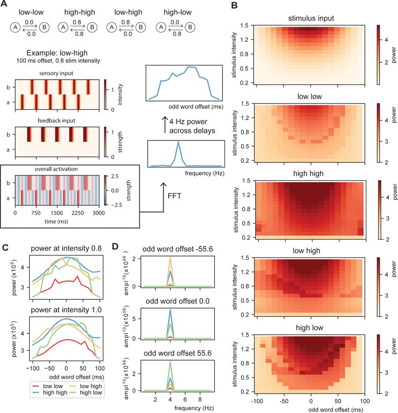
ing within the model will be more or less rhythmic. To do this, we create stimulus input of 10
sequential words at a base rate of 4 Hz to the model with constant (Figure 6A; low at 0 and high at
0.8 predictability) or alternating word-to-word predictability. For the alternating conditions, word-to-
word predictability alternates between low and high (sequences which word are predicted at 0 or
0.8 predictability, respectively) or shift from high to low. For this simulation, we used Gaussian sen-
sory input (with a standard deviation of 42 ms aligning the mean at the peak of the ongoing oscilla-
tion; see Figure 6—figure supplement 1 for output with linear sensory input). Then, we vary the
onset time of the odd words in the sequence (shifting from 100 up to +100 ms) and the stimulus
intensity (from 0.2 to 1.5). We extracted the overall activity of the model and computed the FFT of
the created time course (using a Hanning taper only including data from 0.5 to 2.5 s to exclude the
onset responses). From this FFT, we extracted the peak activation at the stimulation rate of 4 Hz.
The first thing that is evident is that the model with no content predictions has overall lowest
power, but has the strongest 4 Hz response around isochronous presentation (odd word offset of 0
ms) at high stimulus intensities (Figure 6B–D) following closely the acoustic input. Adding overall
high predictability increases the power, but also here the power seems symmetric around zero. The
spectra of the alternating predictability conditions look different. For the low to high predictability
condition, the curve seems to be shifted to the left such that 4 Hz power is strongest when the pre-
dictable odd stimulus is shifted to an earlier time point (low–high condition). This is reversed for the
high–low condition. At middle stimulus intensities, there is a specific temporal specificity window at
which the 4 Hz power is particularly strong. This window is earlier for the low–high than the high–low
alternation (Figure 6C,D and Figure 6—figure supplement 2). The effect only occurs at specific
middle-intensity combination as at high intensities the stimulus dominates the responses and at low
intensities the stimulus does not reach threshold activation. These results show that even though
stimulus input is non-isochronous, the interaction with the internal model can still create a potential
isochronous structure in the brain (see Meyer et al., 2019; Meyer et al., 2020). Note that the direc-
tion in which the brain response is more isochronous matches with the natural onset delays in speech
(shorter onset delays for more predictable stimuli).
Model validation
STiMCON’s sinusoidal modulations of RNN predictions is optimally
sensitive to natural onset delays
Next, we aimed to investigated whether STiMCON would be optimally sensitive to speech input tim-
ings found naturally in speech. Therefore, we tried to fit STIMCON’s expected word-to-word onset
differences to the word-to-word onset differences we found in the CGN. At a stable level of intensity
of the input and inhibition, the only aspect that changes the timing of the interaction between top-
down predictions and bottom-up input within STiMCON is the ongoing oscillation. Considering that
we only want to model for individual words how much the prediction Clþ1!l Alþ1;T ) influences the
expected timing we can set the contribution of the other factors from Equation (1) to zero remain-
ing with the relative contribution of prediction:
Clþ1!l Alþ1;T ¼ top down in fluence ¼ oscðT Þ (4)
We can solve this formula in order to investigate the expected relative time shift (T) in processing
that is a consequence of the strength of the prediction (ignoring that in the exact timing will also
depend on the strength of the input and inhibition):
1 Clþ1!l Alþ1;T
relative time shift ¼ arcsin ’ (5)
2p! Am
w was set as the syllable rate for each sentence, and Am and j were systematically varied. We fitted
a linear model between the STiMCON’s expected time and the actual word-to-word onset
ten Oever and Martin. eLife 2021;10:e68066. DOI: https://doi.org/10.7554/eLife.68066 12 of 25Research article Neuroscience Figure 6. Model output on rhythmicity. (A) We presented the model with repeating (A, B) stimuli with varying internal models. We extracted the power spectra and peak activity at various odd stimulus offsets and stimulus intensities. (B) Strength of 4 Hz power depends on predictability in the stream. When predictability is alternated between low and high, activation is more rhythmic when the predictable odd stimulus arrives earlier and vice versa. (C) Power across different internal models at intensity of 0.8 and 1.0 (different visualization than B). (D) Magnitude spectra at three different odd word offsets at 1.0 intensity. To more clearly illustrate the differences, the magnitude to the power of 20 is plotted. The online version of this article includes the following figure supplement(s) for figure 6: Figure supplement 1. Power at 4 Hz using linearly increasing sensory input. Figure supplement 2. Example of overall activation at threshold 0.8 (Gaussian shaped input). ten Oever and Martin. eLife 2021;10:e68066. DOI: https://doi.org/10.7554/eLife.68066 13 of 25
Research article                                                                                                           Neuroscience

                                   differences. This model was similar to the model described in the section Word-by-word predictabil-
                                   ity predicts word onset differences and included the predictor syllable rate and duration of the previ-
                                   ous word. However, as we were interested in how well non-transformed data matches the natural
                                   onset timings, we did not perform any normalization besides Equation (5). As this might involve vio-
                                   lating some of the assumptions of the ordinary least square fit, we estimate model performance by
                                   repeating the regression 1000 times fitting it on 90% of the data (only including the test data from
                                   the RNN) and extracting R2 from the remaining 10%.
                                       Results show a modulation of the R2 dependent on the amplitude and phase offset of the oscilla-
                                   tion (Figure 7A). This was stronger than a model in which transformation in Equation (5) was not
                                   applied (R2for a model with no transfomation was 0.389). This suggests that STiMCON expected
                                   time durations matches the actual word-by-word duration. This was even more strongly so for spe-
                                   cific oscillatory alignments (around 0.25p offset), suggesting an optimal alignment phase relative to
                                   the ongoing oscillation is needed for optimal tracking (Giraud and Poeppel, 2012; Schroeder and
                                   Lakatos, 2009). Interestingly, the optimal transformation seemed to automatically alter a highly
                                   skewed prediction distribution (Figure 7B) toward a more normal distribution of relative time shifts
                                   (Figure 7C). Note that the current prediction only operated on the word node (to which we have the
                                   RNN predictions), while full temporal shifts are probably better explained by word, syllabic, and
                                   phrasal predictions.

                                   STiMCON can explain perceptual effects in speech processing
                                   Due to the differential feedback strength and the inhibition after suprathreshold feedback stimula-
                                   tion, STiMCON is more sensitive to lower predictable stimuli at phases later in the oscillatory cycle.
                                   This property can explain two illusions that have been reported in the literature, specifically, the
                                   observation that the interpretation of ambiguous input depends on the phase of presentation
                                   (Ten Oever and Sack, 2015; Kayser et al., 2016; Ten Oever et al., 2020) and on speech rate
                                   (Bosker and Reinisch, 2015). The only assumption that has to be made is that there is an uneven
                                   base prediction balance between the ways the ambiguous stimulus can be interpreted.
                                      The empirical data we aim to model comprises an experiment in which ambiguous syllables,
                                   which could either be interpreted as /da/ or /ga/, were presented (Ten Oever and Sack, 2015). In

                                   Figure 7. Fit between real and expected time shift dependent on predictability. (A) Phase offset and amplitude of
                                   the oscillation modulate the fit to the word-to-word onset durations. (B) Histogram of the predictions created by
                                   the deep neural net. (C) Histogram of the relative time shift transformation at phase of 0.15p and amplitude of
                                   1.5.

ten Oever and Martin. eLife 2021;10:e68066. DOI: https://doi.org/10.7554/eLife.68066                                                       14 of 25
Research article Neuroscience
one of the experiments in this study, broadband simuli were presented at specific rates to entrain
ongoing oscillations. After the last entrainment stimulus, an ambiguous /daga/ stimulus was pre-
sented at different delays (covering two cycles of the presentation rate at 12 different steps), puta-
tively reflecting different oscillatory phases. Dependent on the delay of stimulation participants
perceived either /da/ or /ga/, suggesting that phase modulates the percept of the participants.
Besides this behavioral experiment, the authors also demonstrated that the same temporal dynamics
were present when looking at ongoing EEG data, showing that the phase of ongoing oscillations at
the onset of ambiguous stimulus presentation determined the percept (Ten Oever and Sack, 2015).
To illustrate that STiMCON is capable of showing a phase (or delay) dependent effect, we use an
internal language model similar to our original model (Table 2). The model consists of four nodes
(N1, N2, Nda, and Nga). N1 and N2 represent nodes responsive to two stimulus S1 and S2 that func-
tion as entrainment stimuli. N1 activation predicts a second unspecific stimulus (S2) represented by
N2 at a predictability of 1. N2 activation predicts either da or ga at 0.2 and 0.1 probability, respec-
tively. This uneven prediction of /da/ and /ga/ is justified as /da/ is more prevalent in the Dutch lan-
guage as /ga/ (Zuidema, 2010), and it thus has a higher predicted level of occurring. Then, we
present STiMCON (same parameters as before) with /S1 S2 XXX/. XXX is varied to have different
proportion of the stimulus /da/ and /ga/ (ranging from 0% /da/ to 100% /ga/ in 12 times steps; these
reflect relative proportions that sum up to one such that at 30% the intensity of /da/ would be at
max 0.3 and of /ga/ 0.7) and is the onset is varied relate to the second to last word. We extract the
time that a node reaches suprathreshold activity after stimulus onset. If both nodes were active at
the same time, the node with the highest total activation was chosen. Results showed that for some
ambiguous stimuli, the delay determines which node is activated first, modulating the ultimate per-
cept of the participant (Figure 8A, also see Figure 8—figure supplement 1A). The same type of
simulation can explain how speech rate can influence perception (Figure 8—figure supplement 1B;
but see Bosker and Kösem, 2017).
To further scrutinize on this effect, we fitted our model to the behavioral data of Ten Oever and
Sack, 2015. As we used an iterative approach in the simulations of the model, we optimized the
model using a grid search. We varied the parameters of proportion of the stimulus being /da/ or /
ga/ (ranging between 10:5:80%), the onset time of the feedback (0.1:0.1:1.0 cycle), the speed of the
feedback decay (0:0.01:0.1), and a temporal offset of the final sound to account for the time it takes
to interpret a specific ambiguous syllable (ranging between 0.05:0.01:0.05 s). Our first outcome
variable was the node that show the first suprathreshold activation (Nda = 1, Nga = 0). If both nodes
were active at the same time, the node with the highest total activates was chosen. If both nodes
had equal activation or never reached threshold activation, we coded the outcome to 0.5 (i.e., fully
ambiguous). These outcomes were fitted to the behavioral data of the 6.25 Hz and 10 Hz presenta-
tion rate (the two rates showing a significant modulation of the percept). This data was normalized
to have a range between 0 and 1 to account for the model outcomes being binary (0, 0.5, or 1). As a
second outcome measure, we also extracted the relative activity of the /da/ and /ga/ nodes by sub-
tracting their activity and dividing by the summed activity. The activity was calculated as the average
activity over a window of 500 ms after stimulus onset and the final time course was normalized
between 0 and 1.
For the first node activation analysis, we found that our model could fit the data at an average
explained variance of 43% (30% and 58% for 6.25 Hz and 10 Hz, respectively; Figure 8C,D). For the
average activity analysis, we found a fit with 83% explained variance. Compared to the original sinus
fit, this explained variance was higher for the average activation analysis (40% for three parameter
sinus fit [amplitude, phase offset, and mean]). Note that for the first node activation analysis, our fit
cannot account for variance ranging between 0–0.5 and 0.5–1, while the sinus fit can do this. If we
correct for this (by setting the sinus fit to the closest 0, 0.5, or 1 value and doing a grid search to
optimize the fitting), the average fit of the sinus is 21%. Comparing the fits of the rectified sinus ver-
sus the first node activation reveals an average Akaike information criterion of the model and sinus
fits of 27.0 and 24.1, respectively. For the average activation analysis, this was 41.5 versus
27.8, respectively. This overall suggests that the STiMCON model has the better fit. Thus, STiM-
CON does better than a fixed-frequency sinus fit. This is a likely consequence of the sinus fit not
being able to explain the dampening of the oscillation later (i.e., the perception bias is stronger for
shorter compared to longer delays).
ten Oever and Martin. eLife 2021;10:e68066. DOI: https://doi.org/10.7554/eLife.68066 15 of 25Research article Neuroscience
Figure 8. Results for /daga/ illusions. (A) Modulations due to ambiguous input at different times. Illustration of the node that is active first. Different
proportions of the /da/ stimulus show activation timing modulations at different delays. (B) Summary of the model and the parameters altered for the
empirical fits in (C) and (D). (C). R2 for the grid search fit of the full model using the first active node as outcome variable, a model without inhibition (no
inhib), without uneven feedback (no fb), or without an oscillation (no os). The right panel shows the fit of the full model on the rectified behavioral data
of Ten Oever and Sack, 2015. Blue crossed indicate rectified data and red lines indicate the fit. (D) is the same as (C) but using the average activity
instead of the first active node. Removing the oscillation results in an R2 less than 0.
The online version of this article includes the following figure supplement(s) for figure 8:
Figure supplement 1. Explaining speech timing illusions.
Finally, we investigated the relevance of the three key features of our model for this fit: inhibition,
feedback, and oscillations (Figure 8B). We repeated the grid search fit but set either the inhibition
to zero, the feedback matrix equal for both /da/ and /ga/ (both 0.15), or the oscillation at an ampli-
tude of zero. Results showed for both outcome measures that the full model showed the best per-
formance. Without the oscillation, the models could not even fit better than the mean of the model
(R2 < 0). Removing the feedback had a negative influence on both the outcome measures, dropping
the performance. Removing the inhibition reduced performance for both outcome measures, but
more strongly on the average activation compared to the first active node model. This suggest that
all features (with potentially to a lesser extend the inhibition) are required to model the data, sug-
gesting that oscillatory tracking is dependent on linguistic constrains flowing from the internal lan-
guage model.
Discussion
In the current paper, we combined an oscillating computational model with a proxy for linguistic
knowledge, an internal language model, in order to investigate the model’s processing capacity for
onset timing differences in natural speech. We show that word-to-word speech onset differences in
natural speech are indeed related to predictions flowing from the internal language model (esti-
mated through an RNN). Fixed oscillations aligned to the mean speech rate are robust against
ten Oever and Martin. eLife 2021;10:e68066. DOI: https://doi.org/10.7554/eLife.68066 16 of 25Research article Neuroscience
natural temporal variations and even optimized for temporal variations that match the predictions
flowing from the internal model. Strikingly, when the pseudo-rhythmicity in speech matches the pre-
dictions of the internal model, responses were more rhythmic for matched pseudo-rhythmic com-
pared to isochronous speech input. Our model is optimally sensitive to natural speech variations,
can explain phase-dependent speech categorization behavior (Ten Oever and Sack, 2015;
Thézé et al., 2020; Reinisch and Sjerps, 2013; Ten Oever et al., 2020), and naturally comprises a
neural phase code (Panzeri et al., 2015; Mehta et al., 2002; Lisman and Jensen, 2013). These
results show that part of the pseudo-rhythmicity of speech is expected by the brain and it is even
optimized to process it in this manner, but only when it follows the internal model.
Speech timing is variable, and in order to understand how the brain tracks this pseudo-rhythmic
signal, we need a better understanding of how this variability arises. Here, we isolated one of the
components explaining speech time variation, namely, constraints that are posed by an internal lan-
guage model. This goes beyond extracting the average speech rate (Ding et al., 2017;
Poeppel and Assaneo, 2020; Pellegrino and Coupé, 2011) and might be key to understanding
how a predictive brain uses temporal cues. We show that speech timing depends on the predictions
made from an internal language model, even when those predictions are highly reduced to be as
simple as word predictability. While syllables generally follow a theta rhythm, there is a systematic
increase in syllabic rate as soon as more syllables are in a word. This is likely a consequence of the
higher close probability of syllables within a word which reduces the onset differences of the later
uttered syllables (Thompson and Newport, 2007). However, an oscillatory model constrained by an
internal language model is sensitive to these temporal variations, it is actually capable of processing
them optimally.
The oscillatory model we here pose has three components: oscillations, feedback, and inhibition.
The oscillations allow for the parsing of speech and provide windows in which information is proc-
essed (Giraud and Poeppel, 2012; Ghitza, 2012; Peelle and Davis, 2012; Martin and Doumas,
2017). Importantly, the oscillation acts as a temporal filter, such that the activation time of any
incoming signal will be confined to the high excitable window and thereby is relatively robust against
small temporal variations (Figure 5C). The feedback allows for differential activation time dependent
on the sensory input (Figure 5B). As a consequence, the model is more sensitive to higher predict-
able speech input and therefore active earlier on the duty cycle (this also means that oscillations are
less robust against temporal variations when the feedback is very strong). The inhibition allows for
the network to be more sensitive to less predictable speech units when they arrive later (the higher
predictable nodes get inhibited at some point on the oscillation; best illustrated by the simulation in
Figure 8A). In this way, speech is ordered along the duty cycle according to its predictability
(Lisman and Jensen, 2013; Jensen et al., 2012). The feedback in combination with an oscillatory
model can explain speech rate and phase-dependent content effects. Moreover, it is an automatic
temporal code that can use time of activation as a cue for content (Mehta et al., 2002). Note that
previously we have interpreted the /daga/ phase-dependent effect as a mapping of differences
between natural audio-visual onset delays of the two syllabic types onto oscillatory phase
(Ten Oever et al., 2013; Ten Oever and Sack, 2015). However, the current interpretation is not
mutually exclusive with this delay-to-phase mapping as audio-visual delays could be bigger for less
frequent syllables. The three components in the model are common brain mechanisms
(Malhotra et al., 2012; Mehta et al., 2002; Buzsáki and Draguhn, 2004; Bastos et al., 2012;
Michalareas et al., 2016; Lisman, 2005) and follow many previously proposed organization princi-
ples (e.g., temporal coding and parsing of information). While we implement these components on
an abstract level (not veridical to the exact parameters of neuronal interactions), they illustrate how
oscillations, feedback, and inhibition interact to optimize sensitivity to natural pseudo-rhythmic
speech.
The current model is not exhaustive and does not provide a complete explanation of all the
details of speech processing in the brain. For example, it is likely that the primary auditory cortex is
still mostly modulated by the acoustic pseudo-rhythmic input and only later brain areas follow more
closely the constraints posed by the language model of the brain. Moreover, we now focus on the
word level, while many tracking studies have shown the importance of syllabic temporal structure
(Giraud and Poeppel, 2012; Ghitza, 2012; Luo and Poeppel, 2007) as well as the role of higher
order linguistic temporal dynamics (Meyer et al., 2019; Kaufeld et al., 2020b). It is likely that pre-
dictive mechanisms also operate on these higher linguistic levels as well as on syllabic levels. It is
ten Oever and Martin. eLife 2021;10:e68066. DOI: https://doi.org/10.7554/eLife.68066 17 of 25Research article Neuroscience
known, for example, that syllables are shortened when the following syllabic content is known versus
producing syllables in isolation (Pluymaekers et al., 2005a; Lehiste, 1972). Interactions also occur
as syllables part of more frequent words are generally shortened (Pluymaekers et al., 2005b).
Therefore, more hierarchical levels need to be added to the current model (but this is possible fol-
lowing Equation (1)). Moreover, the current model does not allow for phase or frequency shifts. This
was intentional in order to investigate how much a fixed oscillator could explain. We show that onset
times matching the predictions from the internal model can be explained by a fixed oscillator proc-
essing pseudo-rhythmic input. However, when the internal model and the onset timings do not
match, the internal model phase and/or frequency shift are still required and need to be incorpo-
rated (see e.g. Rimmele et al., 2018; Poeppel and Assaneo, 2020).
We aimed to show that a stable oscillator can be sensitive to temporal pseudo-rhythmicities when
these shifts match predictions from an internal linguistic model (causing higher sensitivity to these
nodes). In this way, we show that temporal dynamics in speech and the brain cannot be isolated
from processing the content of speech. This is in contrast with other models that try to explain how
the brain deals with pseudo-rhythmicity in speech (Giraud and Poeppel, 2012; Rimmele et al.,
2018; Doelling et al., 2019). While some of these models discuss that higher-level linguistic proc-
essing can modulate the timing of ongoing oscillations (Rimmele et al., 2018), they typically do not
consider that in the speech signal itself the content or predictability of a word relates to the timing
of this word. Phase resetting models typically deal with pseudo-rhythmicity by shifting the phase of
ongoing oscillations in response to a word that is offset to the mean frequency of the input
(Giraud and Poeppel, 2012; Doelling et al., 2019). We believe that this cannot explain how the
brain uses what/when dependencies in the environment to infer the content of the word (e.g., later
words are likely a less predictable word). Our current model does not have an explanation of how
the brain can actually entrain to an average speech rate. This is much better described in dynamical
systems theories in which this is a consequence of the coupling strength between internal oscillations
and speech acoustics (Doelling et al., 2019; Assaneo et al., 2021). However, these models do not
take top-down predictive processing into account. Therefore, the best way forward is likely to
extend coupling between brain oscillations and speech acoustics (Poeppel and Assaneo, 2020),
with the coupling of brain oscillations to brain activity patterns of internal models (Cumin and Uns-
worth, 2007).
In the current paper, we use an RNN to represent the internal model of the brain. However, it is
unlikely that the RNN captures the wide complexities of the language model in the brain. The deca-
des-long debates about the origin of a language model in the brain remains ongoing and controver-
sial. Utilizing the RNN as a proxy for our internal language model makes a tacit assumption that
language is fundamentally statistical or associative in nature, and does not posit the derivation or
generation of knowledge of grammar from the input (Chater, 2001; McClelland and Elman, 1986).
In contrast, our brain could as well store knowledge of language that functions as fundamental inter-
pretation principles to guide our understanding of language input (Martin, 2016; Martin, 2020;
Hagoort, 2017; Martin and Doumas, 2017; Friederici, 2011). Knowledge of language and linguis-
tic structure could be acquired through an internal self-supervised comparison process extracted
from environmental invariants and statistical regularities from the stimulus input (Martin and Dou-
mas, 2019; Doumas et al., 2008; Doumas and Martin, 2018). Future research should investigate
which language model can better account for the temporal variations found in speech.
A natural feature of our model is that time can act as a cue for content implemented as a phase
code (Lisman and Jensen, 2013; Jensen et al., 2012). This code unravels as an ordered list of
predictability strength of the internal model. This idea diverges from the idea that entrainment
should align to the most excitable phase of the oscillation with the highest energy in the acoustics
(Giraud and Poeppel, 2012; Rimmele et al., 2018). Instead, this type of phase coding could
increase the brain representational space to separate information content (Lisman and Jensen,
2013; Panzeri et al., 2001). We predict that if speech nodes have a different base activity, ambigu-
ous stimulus interpretation should dependent on the time/phase of presentation (see Ten Oever
and Sack, 2015; Ten Oever et al., 2020). Indeed, we could model two temporal speech illusions
(Figure 8, Figure 8—figure supplement 1). There have also been null results regarding the influ-
ence of phase on ambiguous stimulus interpretation (Bosker and Kösem, 2017; Kösem et al.,
2016). For the speech rate effect, when modifying the time of presentation with a neutral entrainer
(summed sinusoidals with random phase), no obvious phase effect was reported (Bosker and
ten Oever and Martin. eLife 2021;10:e68066. DOI: https://doi.org/10.7554/eLife.68066 18 of 25You can also read