A standard protocol for describing individual-based and agent-based models
←
→
Page content transcription
If your browser does not render page correctly, please read the page content below
e c o l o g i c a l m o d e l l i n g 1 9 8 ( 2 0 0 6 ) 115–126

                                              available at www.sciencedirect.com

                                  journal homepage: www.elsevier.com/locate/ecolmodel

A standard protocol for describing individual-based and
agent-based models

Volker Grimm a,∗ , Uta Berger b , Finn Bastiansen a , Sigrunn Eliassen c , Vincent Ginot d ,
Jarl Giske c , John Goss-Custard e , Tamara Grand f , Simone K. Heinz c , Geir Huse g ,
Andreas Huth a , Jane U. Jepsen a , Christian Jørgensen c , Wolf M. Mooij h , Birgit Müller a ,
Guy Pe’er i , Cyril Piou b , Steven F. Railsback j , Andrew M. Robbins k , Martha M. Robbins k ,
Eva Rossmanith l , Nadja Rüger a , Espen Strand c , Sami Souissi m , Richard A. Stillman e ,
Rune Vabø g , Ute Visser a , Donald L. DeAngelis n
a UFZ Umweltforschungszentrum Leipzig-Halle GmbH, Department Ökologische Systemanalyse, Permoserstr. 15, 04318 Leipzig,
Germany
b Zentrum für Marine Tropenökologie, Fahrenheitstr. 6, 28359 Bremen, Germany
c University of Bergen, Department of Biology, P.O. Box 7800, N-5020 Bergen, Norway
d INRA, Unité de Biométrie, Domaine St.-Paul, 84 814 Avignon Cedex 9, France
e Centre for Ecology and Hydrology, Winfrith Technology Centre, Dorchester DT2 8ZD, UK
f 108 Roe Drive, Port Moody, British Columbia V3H 3M8, Canada
g Institute of Marine Research, Box 1870, Nordnes, N-5817 Bergen, Norway
h Netherlands Institute of Ecology, Centre for Limnology, Rijksstraatweg 6, 3631 AC Nieuwersluis, Netherlands
i Hebrew University of Jerusalem, Institute of Life Sciences, Department of Evolution, Systematics and Ecology, Givat Ram Campus,

Jerusalem 91904, Israel
j Lang, Railsback & Associates, 250 California Ave., Arcata, CA 95521, USA
k Max Planck Institute for Evolutionary Anthropology, Deutscher Platz 6, 04103 Leipzig, Germany
l Universität Potsdam, Institut für Biochemie und Biologie, Maulbeerallee 2, 14469 Potsdam, Germany
m Université des Sciences et Technologies de Lille, Station Marine de Wimereux, Ecosystem Complexity Research Group,

CNRS—UMR 8013 ELICO, 28 Avenue Foch BP 80, F-62930 Wimereux, France
n USGS/Florida Integrated Science Centers and Department of Biology, University of Miami, P.O. Box 249118, Coral Gables, FL 33124, USA

a r t i c l e       i n f o                   a b s t r a c t

Article history:                              Simulation models that describe autonomous individual organisms (individual based
Received 8 November 2005                      models, IBM) or agents (agent-based models, ABM) have become a widely used tool, not
Received in revised form 24 April             only in ecology, but also in many other disciplines dealing with complex systems made up of
2006                                          autonomous entities. However, there is no standard protocol for describing such simulation
Accepted 26 April 2006                        models, which can make them difficult to understand and to duplicate. This paper presents
Published on line 14 June 2006                a proposed standard protocol, ODD, for describing IBMs and ABMs, developed and tested by
                                              28 modellers who cover a wide range of fields within ecology. This protocol consists of three
Keywords:                                     blocks (Overview, Design concepts, and Details), which are subdivided into seven elements:
Individual-based model                        Purpose, State variables and scales, Process overview and scheduling, Design concepts, Ini-
Agent-based model                             tialization, Input, and Submodels. We explain which aspects of a model should be described
Model description                             in each element, and we present an example to illustrate the protocol in use. In addition,
Scientific communication                       19 examples are available in an Online Appendix. We consider ODD as a first step for estab-
Standardization                               lishing a more detailed common format of the description of IBMs and ABMs. Once initiated,

    ∗
   Corresponding author. Tel.: +49 341 235 2903; fax: +49 341 235 3500.
   E-mail address: volker.grimm@ufz.de (V. Grimm).
0304-3800/$ – see front matter © 2006 Elsevier B.V. All rights reserved.
doi:10.1016/j.ecolmodel.2006.04.023
116                                       e c o l o g i c a l m o d e l l i n g 1 9 8 ( 2 0 0 6 ) 115–126

                                            the protocol will hopefully evolve as it becomes used by a sufficiently large proportion of
                                            modellers.
                                                                                                            © 2006 Elsevier B.V. All rights reserved.

1.      Introduction                                                        expectation of a familiar structure. As a consequence, we have
                                                                            to read the entire model description in every detail, even if
Simulation models that describe individual organisms or,                    at first we only want to have a general idea of the model’s
more generally, “agents”, have become a widely used tool, not               purpose, structure and processes. This makes reading many
only in ecology (DeAngelis and Gross, 1992; DeAngelis and                   IBM descriptions cumbersome and inefficient. Moreover, if we
Mooij, 2005; Grimm, 1999; Grimm and Railsback, 2005; Huse                   want to critically assess a model or re-implement it, wholly or
et al., 2002; Shugart et al., 1992; Van Winkle et al., 1993) but            in part, we must tediously transform the verbal model descrip-
also in many other disciplines dealing with complex systems                 tion into explicit equations, rules, and schedules before imple-
made up of autonomous entities, including the social sciences               menting it in our own program. Even the many clear and useful
(Epstein and Axtell, 1996; Gilbert and Troitzsch, 2005), eco-               IBM descriptions that certainly exist do not entirely solve the
nomics (Tesfatsion, 2002), demography (Billari and Prskawetz,               communication problem because different authors use differ-
2003), geography (Parker et al., 2003), and political sciences              ent protocols. Thus, a priori, we do not know where in the
(Axelrod, 1997; Huckfeldt et al., 2004). Individual-based models            model description we should expect to find particular infor-
(IBMs) allow researchers to study how system level properties               mation.
emerge from the adaptive behaviour of individuals (Railsback,                   Lengthy verbal descriptions are the second reason why
2001; Strand et al., 2002) as well as how, on the other hand,               many IBM descriptions are so cumbersome. Often we find
the system affects individuals. IBMs are important both for                 a mixture of general considerations, verbal descriptions of
theory and management because they allow researchers to                     processes, and lengthy justifications of the specific model
consider aspects usually ignored in analytical models: vari-                formulations chosen. All this makes it hard to extract the
ability among individuals, local interactions, complete life                information relevant for understanding and implementing the
cycles, and in particular individual behaviour adapting to the              model. But this need not be. Three very successful IBMs, which
individual’s changing internal and external environment.                    have been re-used and modified in numerous follow-up mod-
   However, the great potential of IBMs comes at a cost. IBMs               els, describe their basic model processes in equations: the
are necessarily more complex in structure than analytical                   JABOWA forest model of Botkin et al. (1972) and Shugart (1984),
models. They have to be implemented and run on comput-                      which gave rise to a full pedigree of so-called “gap models”
ers. IBMs are more difficult to analyze, understand and com-                 (Liu and Ashton, 1995); the fish cohort model of DeAngelis et
municate than traditional analytical models (Grimm et al.,                  al. (1980), which initiated large research projects using IBMs
1999). Particularly critical is the problem of communication.               (Tyler and Rose, 1994; Van Winkle et al., 1993); and the fish
Analytical models are easy to communicate because they are                  school model of Huth and Wissel (1992, 1994), which was inde-
formulated in the general language of mathematics. Their                    pendently re-implemented and modified several times (e.g.,
description usually is complete, unambiguous and accessible                 Inada and Kawachi, 2002; Kunz and Hemelrijk, 2003; Reuter
to the reader. In contrast, published descriptions of IBMs are              and Breckling, 1994). The success of these three models seems
often hard to read, incomplete, ambiguous, and therefore less               to a large degree to be due to the fact that their extensive use of
accessible. Consequently, the results obtained from an IBM are              the language of mathematics allowed them to be easily repro-
not easily reproduced (Hales et al., 2003). Science, however, is            duced.
based on reproducible observations. Solving the problem of                      We conclude that what we badly need is a standard protocol
how to communicate IBMs can only increase their scientific                   for describing IBMs which combines two elements: (1) a gen-
credibility (Ford, 2000; Lorek and Sonnenschein, 1999).                     eral structure for describing IBMs, thereby making a model’s
   There are two main and interrelated problems with                        description independent of its specific structure, purpose and
descriptions of IBMs: (1) there is no standard protocol for                 form of implementation (Grimm, 2002) and (2) the language of
describing them and (2) IBMs are often described verbally                   mathematics, thereby clearly separating verbal considerations
without a clear indication of the equations, rules, and sched-              from a mathematical description of the equations, rules, and
ules that are used in the model.                                            schedules that constitute the model. Such a protocol could,
   A standard protocol for the description of IBMs would                    once widely used, guide both readers and writers of IBMs.
make reading and understanding them easier because readers                      In this article we propose a standard protocol for describ-
would be guided by their expectations. Gopen and Swan (1990)                ing IBMs (including agent-based models, multi-agent sim-
explain how understanding is facilitated when writers take                  ulation, or multi-agent systems; see Discussion). The basic
readers’ expectations into account: readers are better able to              idea of the protocol was proposed by Grimm and Railsback
absorb information if it is provided in a familiar, meaningful              (2005) and then discussed during an international workshop
structure. For example, when we read a sentence we expect                   on individual-based modelling held in Bergen, Norway, in the
context at the beginning and the point to be stressed at the                spring of 2004. Most participants of that workshop are among
end. Likewise, when we read a paper describing an analyti-                  the authors of this article, leading to 28 authors from seven dif-
cal model, we expect to see several equations and definitions                ferent countries. The work of the authors covers a wide range
of the variables, then a table of parameter values. But when                of fields within ecology (e.g., marine, terrestrial, plant, animal,
we start reading an IBM-based paper we start without the                    behaviour, population, forest, theory, conservation, etc.), and
e c o l o g i c a l m o d e l l i n g 1 9 8 ( 2 0 0 6 ) 115–126 117
that implements the IBM described. This skeleton includes the
declaration of all objects (classes) describing the models enti-
ties (different types of individuals or environments) and the
scheduling of the model’s processes.
The block or element “Design concepts” does not describe
the model itself, but rather describes the general concepts
underlying the design of the model. The purpose of this ele-
ment of the protocol is to link model design to general con-
cepts identified in the field of Complex Adaptive Systems
(Grimm and Railsback, 2005; Railsback, 2001). These concepts
include questions about emergence, the type interactions
among individuals, whether individuals consider predictions
about future conditions, or why and how stochasticity is con-
Fig. 1 – The seven elements of the ODD protocol, which can sidered. By referring to such general design concepts, each
be grouped into the three blocks: Overview, Design individual-based and agent-based model is integrated into the
concepts, and Details. larger framework of the science of Complex Adaptive Systems.
The third part of ODD, Details, includes three elements
(initialization, input, submodels) that present the details that
the authors have altogether been involved in the writing of were omitted in the overview. In particular, the submodels
more than 200 IBM-based papers. implementing the model’s processes are described in detail.
We agreed to test and refine the standard protocol proposed All information required to completely re-implement the
by Grimm and Railsback (2005) by applying it to our own mod- model and run the baseline simulations should be provided
els: every author, or team of co-authors, rewrote one of their here. If space in a journal article is too limited, Online Appen-
existing model descriptions using the new standard protocol. dices or separate publications of the model’s details should be
The set of 19 models used in this test differs widely in scope, provided.
structure, complexity, and implementation details (see Online The logic behind the ODD sequence is: context and gen-
Appendix). As a result of the test applications, the protocol was eral information is provided first (Overview), followed by more
slightly revised. strategic considerations (Design concepts), and finally more
Here, we first present the standard protocol, which Grimm technical details (Details). We can help readers understand our
and Railsback (2005) refer to as the PSPC + 3 protocol. The IBMs by always using this structure: a standard protocol that
abbreviation “PSPC” referred to the initials of first four ele- provides the information in an order that allows the reader to
ments of the protocol (purpose, structure, process, concepts) easily build on their previous understanding. Below, the seven
and “+3” referred to the remaining three elements. In the elements of ODD are described. A template document of the
revised protocol, however, the names of some elements have ODD protocol is provided in the Online Appendix.
been changed. We are therefore using a new acronym, “ODD”,
which stands for the three blocks of elements ‘Overview’, 2.1. Purpose
‘Design concepts’, and ‘Details’ (Fig. 1).
Then we present an example application of the protocol, The purpose of a model has to be stated first because with-
and summarize our experience with test applications in a list out knowing it, readers cannot understand why some aspects
of frequently asked questions which provides practical hints of reality are included while others are ignored. Usually, the
for using the protocol. Finally we discuss both our experience context and purpose of a model are provided in the intro-
with the test applications and ODD’s potentials and limita- duction of an article, but it is nevertheless important to have
tions and how it could contribute to further unification of the a clear, concise and specific formulation of the model’s pur-
formulation and implementation of IBMs. pose because it provides a guide for what to expect in the
model description that follows. Thus, this element informs
about why you need to build a complex model, and what,
2. The ODD protocol in general and in particular, you are going to do with your
model.
The basic idea of the protocol is always to structure the infor-
mation about an IBM in the same sequence (Fig. 1). This 2.2. State variables and scales
sequence consists of seven elements that can be grouped
in three blocks: Overview, Design concepts, and Details (as What is the structure of the model system? For example, what
a mnemonic, this sequence can be referred to as the ODD kind of low-level entities (e.g., individuals, habitat units) are
sequence). The overview consists of three elements (purpose, described in the model? How are they described? What hier-
State variables and scales, process overview and scheduling), archical levels exist? How are the abiotic and biotic environ-
which provide an overview of the overall purpose and struc- ments described? What is the temporal and spatial resolution
ture of the model. Readers very quickly can get an idea of and extent of the model system?
the model’s focus, resolution and complexity. After reading First, the full set of state variables should be described. The
the overview it should be possible to write, in an object- term ‘state variables’ refers to low-level variables that char-
oriented programming language, the skeleton of a program acterize the low-level entities of the model, i.e. individuals or118 e c o l o g i c a l m o d e l l i n g 1 9 8 ( 2 0 0 6 ) 115–126
habitat units. For example, individuals might be characterized In addition, the scheduling of the model processes should
by a number of characteristics: age, sex, social rank, location, be described. This deals with the order of the processes
parents; habitat units might be characterized by location, soil and, in turn, the order in which the state variables are
type, predation risk (for a certain species), percentage cover. updated. More specific questions include: How is time mod-
It is important not to confuse low-level state variables with elled in the IBM—using discrete time steps, continuous time,
auxiliary, or aggregated, variables, such as population size or or both? Is dynamic scheduling used for events that hap-
average food density in a given area. Auxiliary variables con- pen quickly compared to the model’s time step and are
tain information that is deduced from low-level entities and highly dependent on execution order (Grimm and Railsback,
their low-level state variables. Population size, for example, is 2005)? What model processes or events are grouped into
simply the number of individuals; age structure is a histogram actions that are executed together? Do these actions pro-
taken from the age of all individuals; average food density is duce synchronous or asynchronous updating of the state vari-
the average of the amount of food in every habitat unit in a ables? How are actions that actually happen concurrently
given region. In contrast, low-level state variables cannot be in nature executed in the model? What actions are on a
deduced from other low-level state variables, because they are fixed schedule, and in what order? Are some actions exe-
elementary properties of model entities. Age, sex and loca- cuted in random order? What is the basis for these scheduling
tion, for example, cannot be deduced from any other variable decisions?
but are elementary properties of an individual. In other words, In many cases it will be convenient to visualize scheduling
auxiliary variables aggregate information from model entities, by using flow charts. Freeware software is available for produc-
whereas low-level state variables describe elementary proper- ing flow charts, and some accepted conventions of drawing
ties of the model’s entities. flow charts should be followed. Flow charts must, however,
If the set of (low-level) state variables is large, as is the case correspond literally to the flow of processes in the model, oth-
with many IBMs, it should preferably be presented in a table in erwise they make it virtually impossible to re-implement the
which the variables are grouped according to the entities rep- model. In fact, for dynamic scheduling (e.g., Zeigler et al., 2000)
resented in the model (e.g., individuals, habitat units, abiotic flow charts might actually hinder understanding; pseudo-code
environment). Another option is to use class diagrams of the describing the structure of the simulation program is an alter-
Unified Modeling Language (UML; Fowler, 2003). Once readers native (see, for example, Pitt et al., 2003).
know the full set of (low-level) state variables, they have a clear
idea of the model’s structure and resolution, such as the level 2.4. Design concepts
of detail the individuals are described with. It is daunting to
find how difficult it is to extract the full set of state variables The design concepts provide a common framework for design-
from many existing IBM descriptions. ing and communicating IBMs. They are explained in more
Second, the higher-level entities should be described: for detail in Grimm and Railsback (2005) and in the Appendix
example a population consisting of individuals, a community “Design concepts” in the Online Archive; this Appendix also
consisting of populations, or a landscape consisting of habitat includes a more detailed checklist of questions regarding
units. design concepts. Here we only provide a short checklist which
Finally, in addition to the state variables, the scales should be followed when describing (and designing) an IBM.
addressed by the model should be stated, i.e. length of time Those items of the checklist that do not apply should simply
steps and time horizon, size of habitat cells (if the model is be left out in the model description; an example would be if
grid-based), and extent of the model world (if the model is the model includes no collective agents, such as a herd or fam-
spatially explicit). The reason why these scales have been ily group. The sequence of the checklist items – in contrast to
selected should briefly be explained, because choosing the the seven elements of ODD – is not meant to be compulsory
scale is a fundamental decision determining the design of the but may be shuffled if considered necessary.
entire model. The dimensions must be clearly defined for all
parameters and variables in the tables, to avoid confusion and
inconsistencies and allow model reproduction. With spatially Emergence: Which system-level phenomena truly emerge
explicit models that include spatial heterogeneity, a figure rep- from individual traits, and which phenomena are merely
resenting the model area in a typical configuration can be imposed?
useful. Adaptation: What adaptive traits do the model individuals
have which directly or indirectly can improve their poten-
2.3. Process overview and scheduling tial fitness, in response to changes in themselves or their
environment?
To understand an IBM, we must know which environmental Fitness: Is fitness-seeking modelled explicitly or implicitly? If
and individual processes are built into the model; examples explicitly, how do individuals calculate fitness (i.e., what is
are food production, feeding, growth, movement, mortality, their fitness measure)? In agent-based models that do not
reproduction, disturbance events, and management. At this address animals or plants, instead of fitness other “objec-
stage, a verbal, conceptual description of each process and its tives” of the agents should be considered here (e.g. economic
effects is sufficient because the main purpose of this element revenue, pollution control).
of ODD is to give a concise overview. If the number of processes Prediction: In estimating future consequences of their deci-
included in the model is large, a table listing the processes sions, how do individuals predict the future conditions they
might be useful. will experience?e c o l o g i c a l m o d e l l i n g 1 9 8 ( 2 0 0 6 ) 115–126 119
Sensing: What internal and environmental state variables are model formulation was chosen, how the parameters were
individuals assumed to sense or “know” and consider in their determined, etc., do not belong here. If the list of equations
adaptive decisions? and rules is too long, it should be presented in an Online
Interaction: What kinds of interactions among individuals are Appendix.
assumed? 2. A full model description. This version has exactly the same
Stochasticity: Is stochasticicity part of the model? What are structure as the “skeleton” (i.e., the same subtitles and
the reasons? equation numbers), but now each equation and parameter
Collectives: Are individuals grouped into some kind of collec- is verbally explained in full detail and deals with ques-
tive, e.g. a social group? tions such as: What specific assumptions are underlying
Observation: How are data collected from the IBM for testing, the equations and rules? How were parameter values cho-
understanding, and analyzing it? sen? How were submodels tested and calibrated? Ideally,
the two versions of the detailed model description could be
2.5. Initialization presented in the same document, with the more detailed
verbal descriptions hidden to readers in version one but
This deals with such questions as: How are the environment visible in version two. (This technique is partly used in the
and the individuals created at the start of a simulation run, HTML model description of Deutschman et al. (1997) where
i.e. what are the initial values of the state variables? Is initial- readers can chose links providing more detailed informa-
ization always the same, or was it varied among simulations? tion.)
Were the initial values chosen arbitrarily or based on data?
References to those data should be provided. Communicat- For most IBMs, the second version will be too long to be
ing how IBMs are initialized can be important if peers want to included in a journal paper. Grimm and Railsback (2005) sug-
re-implement the IBM and reproduce the simulation experi- gest two solutions to this problem. One is to use the online
ments reported. or electronic archives of the journal; an increasing number of
journals are providing online archives. The other is to publish
2.6. Input the full model description (version two) in an extra paper or a
technical report which is accessible via the Internet.
The dynamics of many IBMs are driven by some environmen-
tal conditions which change over space and time. A typical
example is precipitation, which may vary over time (sea- 3. Sample application of ODD
sons, years) and space (different spatial patterns of rainfall in
different regions), and management, e.g. harvesting regimes Here we present a sample application of ODD to an individual-
(management might also be addressed in the section “sim- based population model of the alpine marmot, Marmota mar-
ulation experiments”, which usually will follow the model mota (Grimm et al., 2003; Dorndorf, 1999). For reasons of space
description). All these environmental conditions are “input”, limitations, we here chose a relatively simple model that
i.e. imposed dynamics of certain state variables. The model describes many processes empirically by using probabilities,
output gives the response of the model to the input. Readers for example ‘mortality’. The Online Appendix contains exam-
need to know what input data are used, how they were gen- ples of much more complex models that represent many pro-
erated and how they can be generated or obtained. To really cesses mechanistically. The following example is a revised
achieve full reproducibility it might be necessary to provide (in version of a model description given in Grimm et al. (2003).
online archives) the input files that you used yourself, includ-
ing even the random number used as seed. 3.1. Purpose
2.7. Submodels The purpose of the model is to understand how the social
behaviour of the marmots – in particular territoriality, repro-
Here, all submodels representing the processes listed above ductive suppression, and hibernation as a group – affects
in “Process overview and scales” are presented and explained population dynamics and in particular extinction risk if pop-
in detail, including the parameterization of the model. But, ulations are small.
given the space limitations of journals, how can we make the
detailed model description easy to understand, easy to use for 3.2. State variables and scales
re-implementing the model, and nevertheless complete? The
answer partly depends on the complexity of the model, but in The model comprises four hierarchical levels: individual, ter-
general we propose that two versions of the detailed model ritory, (meta)population, and environment. Individuals are
description be written: characterized by the state variables: identity number, age, sex,
identity of the territory where the individual lives, and social
1. The mathematical “skeleton” of the model. This skele- rank. Newborns have the additional state variable weaning
ton consists of the model equations and rules and one weight, which affects their mortality. Individuals which have
or more tables presenting the model parameters and their not completed their first winter are referred to as juveniles;
dimensions. Verbal explanations of the equations and rules 1-year-olds as yearlings, and all others as adults. Apart from
should be kept to a minimum: parameters have of course to this, social rank is the main attribute which tells the difference
be explained, but longer explanations of why this specific between dominant and subdominant adults (Table 1).120 e c o l o g i c a l m o d e l l i n g 1 9 8 ( 2 0 0 6 ) 115–126
Table 1 – Overview of processes, parameters and default
values of parameters of the marmot model
Parameter Value
Number of territories 22
Age of sexual maturity (years) 2
Winter mortality
Mean of the winter strength distribution (days) 117
Standard deviation of the winter strength 10.2
distribution (days)
Mean of the territory quality distribution (days) 0
Standard deviation of territory quality distribution 8.4
(days)
Mean of the weaning date distribution (days) 185.5
Standard deviation of the weaning date 6.6
distribution (days)
Winter mortality of floaters 0.9
Recolonization
Dispersal probability at age 2 0.2
Dispersal probability at age 3 0.7
Dispersal probability at age 4 0.5
Dispersal probability at age 5 1
Probability to inherit a vacant dominant position 0.2
at home
Probability to occupy a vacant dominant position 0.3
in the neighbourhood
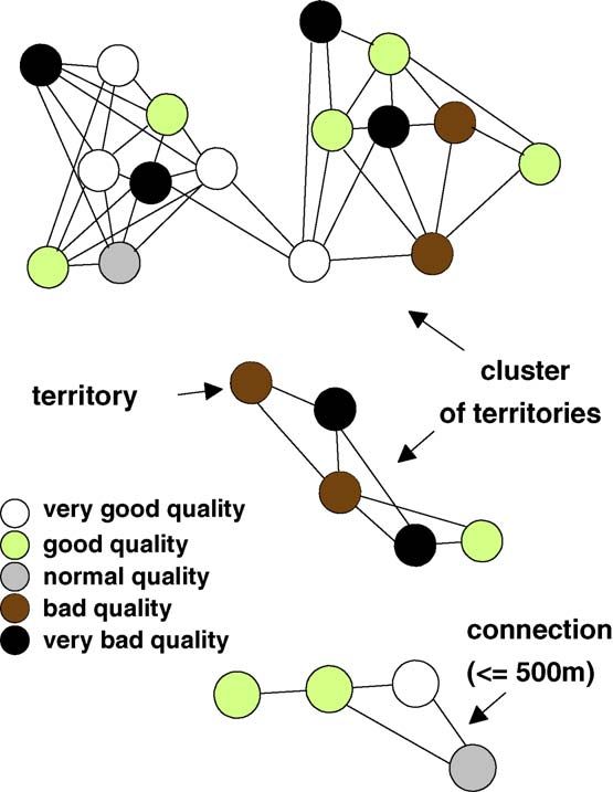
Fig. 2 – Spatial arrangement of territories in the model.
Probability to occupy a vacant dominant position 0.5
Territories which are closer than 500 m to each other are
further away than 500 m
Eviction linked by lines, indicating the chance of subdominants
Eviction probability of dominant animal 0.15 recolonizing vacant dominant positions within this
Reproduction neighbourhood without undertaking long-distance
Reproduction probability of a dominant female 0.64 dispersal. The different grey scales of the territories
Mean of the litter size distribution 3.3 indicate different habitat qualities of the territories (from
Standard deviation of the litter size distribution 1.43
Grimm et al., 2003, after Dorndorf, 1999).
Sex ratio in a litter 0.58
Summer mortality
Summer survival of juveniles 0.9
Summer survival of yearlings 0.94 account by specifying the linkages to neighbouring territories.
A neighbouring territory is defined as a territory within the
If not otherwise specified, these default values are used (from
distance of 500 m. The number of linkages may vary between
Grimm et al., 2003, after Dorndorf, 1999). Dimensionless parame-
ters are either numbers or probabilities; for parameter tables with a zero and six (Fig. 2). Clusters of neighbouring territories com-
stronger focus on the dimensions of the parameters, see examples pose a local metapopulation. Several clusters make up the
in the Online Appendix. regional metapopulation of the alpine marmot (Fig. 2). As dis-
tances between clusters are greater than 500 m, only dispers-
ing subdominants will cross this distance. On this spatial scale
A territory may be occupied by a social group of marmots beyond 500 m the model is not spatially explicit but the dis-
and contains one hibernaculum used by this group during persers may reach any cluster of territories within the model
winter. A territory is characterized by the state variables: iden- area. This restricts the extent of the area that can be described
tity number, the number and list of individuals present, and by the model to several square kilometres.
its quality. If the number of individuals is zero, the territory The highest hierarchical level in the model is the abiotic
is referred to as ‘empty’, i.e. space which has become vacant environment and its fluctuations. Since the severity of win-
due to the extinction of a social group. Thus, territories may ter, indicated by the date when territories become snow-free,
be recolonized just like empty patches in metapopulations. is the most important aspect in the life of marmots, the abi-
‘Quality’ is an attribute characterizing habitat heterogeneity otic environment in the model is characterized by this date.
with respect to the harshness of overwintering conditions, The date when a territory becomes snow-free is referred to as
indicated by the date in spring when a territory becomes snow- ‘winter strength’; it is drawn from a normal distribution and
free. modulated by the quality of the territories.
The population is composed of several territories or social
groups, respectively. Populations are characterized by size, the 3.3. Process overview and scheduling
number of social groups, and the number and list of territories.
In addition, a “floater pool” keeps track of both all subdom- The model proceeds in annual time steps. Within each year or
inants which have left their home territory and dominants time step, seven modules or phases are processed in the fol-
which have been evicted. The spatial structure is taken into lowing order: winter mortality, eviction, inheritance, dispersal,e c o l o g i c a l m o d e l l i n g 1 9 8 ( 2 0 0 6 ) 115–126 121
Fig. 3 – Life history of the model marmots showing the transitions between different age and social classes, as well as the
processes which cause these transitions (from Grimm et al., 2003, after Dorndorf, 1999).
re-colonization of vacant dominant positions, reproduction, describing, for example, mortality and dispersal rates as
and summer mortality. Within each module, individuals and probabilities. Adaptation and fitness-seeking are thus not
territories are processed in a random order. The individuals modelled explicitly, but are included in the empirical rules.
life cycle is depicted in Fig. 3. Sensing: Individuals are assumed to know their own sex, age,
and social rank so that they apply, for example, their age-
3.4. Design concepts specific dispersal probabilities.
Interaction: Three types of interactions are modelled implic-
Emergence: Population dynamics emerge from the behaviour itly: winter mortality decreases with group size, alpha indi-
of the individuals, but the individual’s life cycle and viduals suppress reproduction of subdominants, and after
behaviour are entirely represented by empirical rules changes in the alpha male position in the current year,122 e c o l o g i c a l m o d e l l i n g 1 9 8 ( 2 0 0 6 ) 115–126
the alpha female does not reproduce. One interaction is Similarly, winter mortality for subdominants (including year-
modelled explicitly: subdominants and individuals from the lings) is:
floater pool can try to evict alpha individuals.
Stochasticity: All demographic and behavioural parameters −1
Psub = [1 + exp(7.545 − 0.038WS)] (2)
are interpreted as probabilities, or are drawn from empirical
probability distributions. This was done to include demo- For juveniles, we found in addition a significant influence of
graphic noise and because the focus of the model is on weaning weight on winter mortality:
population-level phenomena, not on individual behaviour.
Winter strength was taken from a truncated normal distri- −1
Pnew = [1 + exp(−1.014 − 0.024WS + 0.008WW + 0.613SUB)]
bution in order to include environmental noise (i.e., variation
of the population’s growth rate driven by fluctuations of abi- (3)
otic conditions). Likewise, habitat quality was taken from a
truncated normal distribution in order to include spatial het- with WW being the weaning weight (see below, Reproduction)
erogeneity. and SUB the number of subdominants (excluding yearlings).
Observation: For model testing, the spatial distribution of Thus, the place where sociality comes into play in our model
the individuals was observed process by process. For model is in Eqs. (1) and (3) via the variable SUB.
analysis, only population-level variables were recorded, i.e. Two additional model rules take into account further pro-
group size distribution, population size over time, and time cesses affecting mortality. Firstly, in groups without sub-
to extinction (using the “ln(1 − P0 ) plot” of Grimm and Wissel, dominants and yearlings, the dominant couple had a higher
2004). risk of mortality than specified by Eq. (1). Whether the first
dominant marmot (which is chosen randomly) dies or sur-
3.5. Initialization vives is determined according to the mortality specified in
Eq. (1). If it dies its partner has an increased probability
Each territory was initially occupied with a 5-year-old couple of dying of P = 0.66. If this partner dies as well, the new-
of dominants and both a 1-year-old male and female sub- borns – if present – will also die in turn. To avoid that this
dominant. The evaluation of each simulation run started in rule introduces a higher total mortality than specified in Eq.
the first year when the number of model adults was equal to (1), for the case that the first partner survives the mortal-
the number of adults observed in the first year of the field ity of the second partner had to be modified (see Online
study. Appendix).
The second model modification concerning winter mortality
3.6. Input introduces the probability PC , which takes into account
the extinction of entire social groups due to local catastro-
In general model analysis, each year winter strength is drawn phes during winter. We use a value of PC = 0.004. Finally, we
from a normal distribution with an empirically determined assume a winter mortality of the floaters which failed to take
mean and standard deviation (mean = 117 days of the year for over a new territory during the summer as Pfloatwinter = 0.9.
territories in the study area, s = 10.2 days). This overall winter Eviction: Dominant positions may become vacant not only
strength is modified by differences in overwintering condi- due to winter mortality but also because the existing dom-
tions among territories, i.e., from a normal distribution with a inant animal has been evicted by a subdominant group
mean of zero and a standard deviation of 8.4 days. This means member or a floater. We assume that dominant individuals
that territories which have a higher quality than the mean are evicted with a probability of PEV = 0.15 and that all evicted
become snow-free a certain number of days earlier than speci- animals enter the floater pool.
fied by the overall winter strength, whereas territories of lower The following three modules of the model describe how dom-
quality become snow-free later. inant positions which became vacant due to winter mortality
and eviction are reoccupied by subdominants or dispersers.
3.7. Submodels Inheritance: The oldest subdominant animal has a probability
of PIN = 0.22 of taking the dominant position. If this animal
Winter mortality: For dominant marmots, winter mortality – fails or if there is no subdominant in the territory, the
interpreted as the probability of dying in a certain winter – dominant position remains vacant and can be taken over by
is determined from the long-term data set by logistic regres- a floater (see below).
sion: Dispersal: Most of the subdominants willing to disperse leave
−1 their home territory in spring. The probability of leaving
Pter = [1 + exp(6.82 − 0.286A − 0.028WS + 0.395SUBY)]
depends on age and is directly taken from Table 2. Dispersed
(1) animals are compiled in a list called the “floater pool”.
This list is used to handle the assignment of free dominant
where A is the age, WS winter strength, and SUBY is the positions to floaters. Note that the floater pool contains both
number of subdominants (including yearlings) present in a true floaters which disperse beyond 500 m and are subject
group. Eq. (1) states that the winter mortality of dominants to dispersal mortality during summer, and animals which
increases with the severity of overwintering conditions and will take over a dominant position in the neighbourhood.
with age, but decreases with the number of subdominants Recolonization: In the model, recolonization is implemented
and yearlings. by the following suite of rules. The first rule decides with ae c o l o g i c a l m o d e l l i n g 1 9 8 ( 2 0 0 6 ) 115–126 123
probability of RN = 0.5 whether a vacant dominant position tal systems (Peck, 2004), and scenarios, sensitivity or uncer-
is reoccupied by a marmot that comes from a neighbouring tainty analysis, etc. are all just that: simulation experiments
territory. If this is the case, the floater pool is searched (in a that are carefully designed to test a certain hypothesis. This
random order) for such an animal, and if no animal is found hypothesis or purpose of the experiment should clearly be
the dominant position remains vacant. After repeating this stated.
procedure for each vacant dominant position, the remaining
animals in the floater pool are treated as true floaters and 4.2. Should the elements of ODD always be presented
have a dispersal mortality of PD = 0.3, i.e. about 30% of the in the given sequence?
remaining floaters die before the next model rules are
applied. Yes, definitely. This is the main idea of the protocol: first pro-
The next rule is analogous to the first rule, but this time viding a comprehensive overview; then explaining the design
each of remaining true floaters is allowed to occupy an concepts underlying the model, and finally presenting all
available dominant position with a probability of RF = 0.5. details that are necessary to fully understand and – in prin-
Finally, the last rule of this module checks territories where ciple – re-implement the model. The sequence of the design
the dominant positions are still unoccupied for the presence concepts, however, may be changed, if considered necessary.
of sexually mature animals. If one is found, the oldest
subdominant animal moves into the dominant position. 4.3. Where do I describe parameterization and tests of
Reproduction: Only when a dominant male and female are the submodels?
present in a territory reproduction can take place. The
probability of a dominant female having offspring is 0.64 In the element “Submodels”. If parameterization was not very
(Hackländer and Arnold, 1999). The mean litter size (L) complex, it might be sufficient to present the source of the
is 3.3 and standard deviation is 1.43. The mean weaning parameters in the table listing the parameters. If parameteri-
weight (WWmean ) is 536 g (S.D. = 126.3 g) but decreases zation was a major issue, it might be best to describe it briefly
with litter size. Therefore a regression model is used to in the article and give details in an Online Appendix. The same
assess a mean weaning weight depending on litter size applies to tests of the submodels, e.g. comparing them to inde-
L (WWmean = 680.23 − 35.24L, R2 = 0.143, P < 0.001). In the pendent implementations using, for example, spreadsheets
model, litter size and weaning weight are drawn from nor- (Grimm and Railsback, 2005).
mal distributions (in the case of litter size, discretized and
truncated to the interval [1,6]) with the means and standard 4.4. What about the source code and the executable
deviations specified. The sex of offspring is determined by program?
chance with a bias of 0.58 towards males. We assume that
no reproduction occurs if the holder of a male dominant Even the most carefully prepared verbal model description is
position has changed during the current year. likely to contain a few ambiguities that make it difficult, or
Summer mortality: Summer mortality rates are only known even impossible, to independently re-implement the model
from the field for juveniles and yearlings. Summer mortality (Edmonds and Hales, 2003; Rouchier, 2003). We therefore rec-
of resident adults is low but hard to quantify. The summer ommend that the source code, or parts of it, be provided in
mortality of adults is thus indirectly and implicitly taken an Online Archive. So far this has not been done very often,
into account in the probabilities of eviction and dispersal partly because authors might want to keep their code propri-
mortality. Newborns and yearlings die during summer with etary, partly because there are so many different programming
a probability of 0.11 and 0.07, respectively. languages, compilers, software platforms, and operation sys-
tems that usually only a minority of readers will be able to
fully understand the code or even run it on their own comput-
4. Practical hints for using ODD ers. It should, however, be possible to communicate how the
three elementary parts of a model have been coded: the dec-
During the test of the protocol, several questions arose that laration of the model’s entitities, the scheduling of processes,
are not answered by the description of the protocol itself. The and the very rules and equations that have been used to repre-
following list of questions is thus organized in the style of “Fre- sent the processes. Even if we, for example, do not understand
quently Asked Questions” (FAQ). We plan to maintain this list Java, it should be possible to check in a Java program how the
on a webpage devoted to ODD. The evolving FAQ could be the three elementary parts of the model have been implemented.
basis of future developments of the protocol. The minimum requirements for this would be: comments that
identify the three elementary parts, the meaning of the pro-
4.1. Are scenarios, simulation experiments, and gram variables, and the purpose of methods, functions, and
sensitivity analysis part of the protocol? procedures.
In addition, it would be good practice to provide an exe-
No. The protocol is designed to describe the basic model. It cor- cutable version of the program that is capable of performing
responds to the “Materials” part of an article presenting empir- all or the most important simulation experiments that are
ical work. We recommend including a section entitled “simu- described in the article. All initialization, input, and output
lation experiments” following the description of the model. files that are required to run the program should be included.
This section would correspond to the classical “Methods” For a detailed discussion of the costs and benefits of providing
part of research articles. Simulation models are experimen- the executable program, see Grimm (2002).124 e c o l o g i c a l m o d e l l i n g 1 9 8 ( 2 0 0 6 ) 115–126
4.5. Why not use the Unified Modeling Language and reporting their results without anyone else reproducing
(UML)? what they found.” (Section 1.2). Reproducing results, however,
is a conditio sine qua non for making simulation models a more
UML is indeed a powerful tool to describe object-oriented soft- rigorous tool for science: “Since almost all simulations are not
ware in a unifying format (Fowler, 2003). However, the full amenable to formal analysis, the only way they can be veri-
UML is quite complex and includes numerous types of dia- fied is via the experimentation of running simulations. If we
grams that are not at all easy to develop or understand. UML are to be able to trust the simulations we use, we must inde-
was designed and is developed by professional software engi- pendently replicate them.” (Edmonds and Hales, 2003, Section
neers. The purpose of ODD, however, was that it can eas- 12.2). A similar point is made by Aber (1997).
ily be written and understood by ecologists, who usually are The ODD protocol is designed as a tool to facilitate the com-
not software engineers. Ultimately, something similar to UML munication and replication of IBMs and agent-based models
should be developed for individual-based and agent-based (ABMs). We consider the protocol as a first step for establishing
models: a visual declarative language that is easy to use and a more detailed common format of the description of IBMs and
can directly be compiled to computer code (tools for translat- ABMs. The test applications of ODD presented in the Online
ing code to UML and vice versa exist). We recommend reading Appendix show that it does not immediately solve all prob-
introductory texts of UML and using the most basic and simple lems of communicating IBMs or ABMs, but is a step in the
type of diagram, the “class diagram” (see examples in Online right direction.
Appendix). Originally, we expected that the protocol as proposed by
Grimm and Railsback (2005) would make the test model
4.6. How to deal with different journal formats? descriptions (Online Appendix) quite similar, but this was less
so than expected for two reasons. First, the original formu-
Journals have different format requirements for headlines, lation of the protocol used a terminology, for example “state
number of headline levels, etc. We recommend trying to use variables”, that was not explicitly defined and therefore vari-
the elements labels (“Purpose”, “State Variables and Scales”) as ously interpreted in the test applications. We tried to remove
headlines, because this provides a clear visual guide to read- this terminological ambiguity in the revised formulation of the
ers. If journals are particular about headlines, the elements protocol. Second, the test situation was somewhat unnatu-
names should be highlighted by other means. ral: existing descriptions of sometimes very complex models
were rearranged and slightly revised, but not newly written
4.7. In models including human agents, where do we from scratch. However, we expect that model descriptions will
describe memory and behavioural strategies? be more homogeneous if written anew, following the protocol
presented above.
Anything that is used to distinguish individuals is considered a Still, as can be seen from the example above and in the
low-level state variable. Memory clearly is represented by such Online Appendix, differences in the style of the presentation
variables. A behavioural strategy is not part of the individual’s are likely to remain. We have to accept this at the current stage,
state if all individuals use the same strategy. If individuals can because the protocol has to compromise between being gen-
have different, but fixed strategies, then a variable indicating eral enough to include all kinds of individual-based or agent-
the strategy used by an individual would be a state variable, based models and being specific enough to fulfil its purpose.
and the set of strategies would be submodels. If behavioural In particular, the protocol is not specific enough to “force” a
strategies vary continuously, then the variables and param- more strict use of the language of mathematics. It is, however,
eters specifying the behaviour of an individual are the state a good exercise to take an existing model description, which
variables characterizing behaviour. usually is a mixture of rules, equations, and lengthy explana-
tion, and to keep only the factual description of the model and
4.8. I find it difficult to clearly describe “scheduling” leave out all motivations, explanations, and justifications.
Besides the current limitations of ODD, however, also the
Of all elements of a model description, “scheduling” is the least benefits of the protocol became obvious in the test applica-
developed one and, in fact, is simply left out in many descrip- tions. The most important benefits were:
tions. Verbal descriptions are usually not sufficient to describe
the ordering of processes in a model. Flow charts certainly are • The model description became easier to write. It was no
useful and easy to grasp, but for any scheduling deviating from longer necessary to waste a lot of time thinking about how
a linear sequence of processes, pseudo code that exactly cor- to structure the text, because the protocol had made those
responds to the code used for simulations should be provided decisions for the authors so that they simply could follow
(plus the code itself). the template.
• The model description became more complete because the
protocol reminded the authors of important details that
5. Discussion they might have otherwise forgotten to include in the doc-
umentation.
Regarding the communication and development of individual- • The model description became easier to understand. In
based or agent-based models, the current situation is one case, for example, the protocol suggested a context for
poignantly described by Hales et al. (2003): “Researchers tend describing a concept that had been confusing to the review-
to work in isolation, designing all their models from scratch ers of the original paper (emergence). If ODD had been usede c o l o g i c a l m o d e l l i n g 1 9 8 ( 2 0 0 6 ) 115–126 125
before, the review process would have been smoother and Billari, F., Prskawetz, A., 2003. Agent-Based Computational
the final description would have been clearer. Demography: Using Simulation to Improve Our
• The protocol is not only useful for individual-based or Understanding of Demographic Behaviour. Springer
Physica-Verlag, Heidelberg.
agent-based models, but for bottom-up simulation mod-
Botkin, D.B., Janak, J.F., Wallis, J.R., 1972. Some ecological
els in general, for example grid-based models. Two of the consequences of a computer model of forest growth. J. Ecol.
test applications (“Biological control”, “Rangeland manage- 60, 849–873.
ment”) are not individual-based; here, those design con- DeAngelis, D.L., Cox, D.K., Coutant, C.C., 1980. Cannibalism and
cepts that did not apply were simply ignored. size dispersal in young-of-the-year largemouth bass:
experiment and model. Ecol. Model. 8, 133–148.
DeAngelis, D.L., Gross, L.J., 1992. Individual-Based Models and
Once ODD is used by a sufficiently large proportion of mod-
Approaches in Ecology. Chapman and Hall, New York.
ellers, the next step would perhaps be to develop more specific
DeAngelis, D.L., Mooij, W.M., 2005. Individual-based modeling of
formats for the seven elements of the protocol. For exam- ecological and evolutionary processes. Annu. Rev. Ecol. Evol.
ple, UML class diagrams could become standard for giving Syst. 36, 147–168.
an overview of state variables and processes; a certain for- Deutschman, D.H., Levin, S.A., Devine, C., Buttel, L., 1997. Scaling
mat of pseudo-code describing process scheduling could be from trees to forests: analysis of a complex simulation model.
developed; a certain style for representing model rules could Science 277, 1688, Available at:
http://www.sciencemag.org/feature/data/deutschman/
be established; or we could even identify a limited set of
index.htm.
“behavioural primitives” (Ginot et al., 2002) that might be mod- Dorndorf, N., 1999. Zur Populationsdynamik des
elled in alternative but compatible ways. Alpenmurmeltiers: Modellierung, Gefährdungsanalyse und
If ODD develops as we envision it, we might after, say, 5–10 Bedeutung des Sozialverhaltens für die Überlebensfähigkeit.
years come to the point where the following vision of the Ph.D. Thesis. Philipps-Universität Marburg, Germany.
IBM developers “software heaven” becomes reality: “modelers Edmonds, B., Hales, D., 2003. Replication, replication, and
replication: some hard lessons from model alignment.
could describe their IBM on paper using some kind of language
J. Artif. Soc. Soc. Simul. 6, http://jasss.soc.surrey.ac.uk/6-4/
that (1) people can understand intuitively, (2) is widely used
11.html.
throughout ecology, (3) provides ‘shorthand’ conventions that Epstein, J., Axtell, R., 1996. Growing Artificial Societies. Social
minimize the effort to describe the IBM rigorously and com- Science from the Bottom Up. Brookins Institution Press/The
pletely, and (4) can be converted directly into an executable MIT Press.
simulator without the possibility of programming errors. After Ford, E.D., 2000. Scientific Method for Ecological Research.
converting the model description into an executable simula- Cambridge University Press, Cambridge.
Fowler, M., 2003. UML Distilled: A Brief Guide to the Standard
tor, the modelers then could turn the simulator into a sim-
Object Modeling Language, third ed. Addison–Wesley
ulation laboratory by attaching experimentation tools: probes
Professional.
to collect data; displays to show results visually; controls Gilbert, N., Troitzsch, K., 2005. Simulation for the Social Scientist,
that automatically generate, execute, and interpret . . . analysis second ed. Open University Press, Milton Keynes.
experiments” (Grimm and Railsback, 2005, p. 271). Ginot, V., Le Page, C., Souissi, S., 2002. A multi-agents architecture
We are planning to maintain an ODD webpage (which will to enhance end-user individual-based modelling. Ecol. Model.
be accessible via http://www.ufz.de/oesatools/odd), to regu- 157, 23–41.
Gopen, G.D., Swan, J.A., 1990. The science of scientific writing.
larly evaluate the usage of the protocol, to collect questions
Am. Sci. 78, 550–559.
and suggestions of users, and to publish new “releases” of the Grimm, V., 1999. Ten years of individual-based modelling in
protocol, which should, however, be compatible with earlier ecology: What have we learned, and what could we learn in
releases. the future? Ecol. Model. 115, 129–148.
Grimm, V., 2002. Visual debugging: a way of analyzing,
understanding, and communicating bottom-up simulation
Acknowledgements models in ecology. Nat. Res. Model. 15, 23–38.
Grimm, V., Dorndorf, N., Frey-Roos, F., Wissel, C., Wyszomirski, T.,
Arnold, W., 2003. Modelling the role of social behavior in the
We would like to thank two anonymous reviewers for helpful persistence of the alpine marmot Marmota marmota. Oikos
comments. 102, 124–136.
Grimm, V., Railsback, S.F., 2005. Individual-Based Modeling and
Ecology. Princeton University Press, Princeton, NJ.
Appendix A. Supplementary data Grimm, V., Wissel, C., 2004. The intrinsic mean time to
extinction: a unifying approach to analyzing persistence and
Supplementary data associated with this article can be found, viability of populations. Oikos 105, 501–511.
Grimm, V., Wyszomirski, T., Aikman, D., Uchmanski, J., 1999.
in the online version, at doi:10.1016/j.ecolmodel.2006.04.023.
Individual-based modelling and ecological theory: synthesis
references of a workshop. Ecol. Model. 115, 275–282.
Hackländer, K., Arnold, W., 1999. Male-caused failure of female
reproduction and its adaptive value in alpine marmots
(Marmota marmota). Behav. Ecol. 10, 592–597.
Aber, J.D., 1997. Why don’t we believe the models? Bull. Ecol. Soc. Hales, D., Rouchier, J., Edmonds, B., 2003. Model-to-model
Am. 78, 232–233. analysis. J. Artif. Soc. Soc. Simul. 6,
Axelrod, R., 1997. The Complexity of Cooperation: Agent-based http://jasss.soc.surrey.ac.uk/6-4/5.html.
Models of Competition and Collaboration. Princeton Huckfeldt, R., Johnson, P.E., Sprague, J.D., 2004. Political
University Press, Princeton, NJ. Disagreement: The Survival of Diverse Opinions withinYou can also read