Ocean carbon cycle feedbacks in CMIP6 models: contributions from different basins
←
→
Page content transcription
If your browser does not render page correctly, please read the page content below
Biogeosciences, 18, 3189–3218, 2021
https://doi.org/10.5194/bg-18-3189-2021
© Author(s) 2021. This work is distributed under
the Creative Commons Attribution 4.0 License.

Ocean carbon cycle feedbacks in CMIP6 models:
contributions from different basins
Anna Katavouta1,2 and Richard G. Williams1
1 Department  of Earth, Ocean and Ecological Sciences, School of Environmental Sciences,
University of Liverpool, Liverpool, UK
2 National Oceanography Centre, Liverpool, UK

Correspondence: Anna Katavouta (a.katavouta@liverpool.ac.uk)

Received: 23 December 2020 – Discussion started: 4 January 2021
Revised: 31 March 2021 – Accepted: 13 April 2021 – Published: 27 May 2021

Abstract. The ocean response to carbon emissions involves          fects of a decrease in solubility and physical ventilation and
the combined effect of an increase in atmospheric CO2 ,            an increase in accumulation of regenerated carbon. The more
acting to enhance the ocean carbon storage, and climate            poorly ventilated Indo-Pacific Ocean provides a small con-
change, acting to decrease the ocean carbon storage. This          tribution to the carbon cycle feedbacks relative to its size. In
ocean response can be characterised in terms of a carbon–          the Atlantic Ocean, the carbon cycle feedbacks strongly de-
concentration feedback and a carbon–climate feedback. The          pend on the AMOC strength and its weakening with warm-
contribution from different ocean basins to these feedbacks        ing. In the Arctic, there is a moderate correlation between
on centennial timescales is explored using diagnostics of          the AMOC weakening and the carbon–climate feedback that
ocean carbonate chemistry, physical ventilation and biolog-        is related to changes in carbonate chemistry. In the Pacific,
ical processes in 11 CMIP6 Earth system models. To gain            Indian and Southern oceans, there is no clear correlation be-
mechanistic insight, the dependence of these feedbacks on          tween the AMOC and the carbon cycle feedbacks, suggesting
the Atlantic Meridional Overturning Circulation (AMOC)             that other processes control the ocean ventilation and carbon
is also investigated in an idealised climate model and the         storage there.
CMIP6 models. For the carbon–concentration feedback, the
Atlantic, Pacific and Southern oceans provide compara-
ble contributions when estimated in terms of the volume-
integrated carbon storage. This large contribution from the        1   Introduction
Atlantic Ocean relative to its size is due to strong local phys-
ical ventilation and an influx of carbon transported from          Carbon emissions drive an Earth system response via direct
the Southern Ocean. The Southern Ocean has large anthro-           changes in the biogeochemical carbon cycle and the physi-
pogenic carbon uptake from the atmosphere, but its contri-         cal climate. These changes in the biogeochemical carbon cy-
bution to the carbon storage is relatively small due to large      cle and physical climate further amplify or dampen the Earth
carbon transport to the other basins. For the carbon–climate       system response, with this amplification often referred to as a
feedback estimated in terms of carbon storage, the Atlantic        feedback (Sherwood et al., 2015). The physical climate feed-
and Arctic oceans provide the largest contributions relative       back involves the combined effect from changes in atmo-
to their size. In the Atlantic, this large contribution is pri-    spheric water vapour, tropospheric lapse rate, surface albedo
marily due to climate change acting to reduce the physical         and clouds (Ceppi and Gregory, 2017) and from a shift in the
ventilation. In the Arctic, this large contribution is associ-     regional patterns of ocean heat uptake due to changes in the
ated with a large warming per unit volume. The Southern            ocean circulation (Winton et al., 2013). For the carbon cycle,
Ocean provides a relatively small contribution to the carbon–      an initial increase in atmospheric CO2 leads to carbon up-
climate feedback, due to competition between the climate ef-       take and storage in land and ocean reservoirs. This response
                                                                   of the carbon cycle to the increase in atmospheric CO2 is

Published by Copernicus Publications on behalf of the European Geosciences Union.
3190 A. Katavouta and R. G. Williams: Ocean carbon cycle feedbacks in CMIP6 models
characterised by the carbon–concentration feedback. At the
same time, the carbon cycle is further modified by changes
in the physical climate, such as warming and an increase in
ocean stratification leading to an amplification of the initial
increase in atmospheric CO2 . This response of the carbon
cycle to changes in the physical climate is characterised by
the carbon–climate feedback. These two carbon cycle feed-
backs have been extensively used to understand and quantify
the response of the global carbon cycle to carbon emissions
(Friedlingstein et al., 2003, 2006; Gregory et al., 2009; Boer
and Arora, 2009; Arora et al., 2013; Schwinger et al., 2014;
Schwinger and Tjiputra, 2018; Williams et al., 2019; Arora
et al., 2020). A regional extension of the carbon cycle feed-
backs has been also used to explore their geographical dis-
tribution and the mechanisms that control the land and ocean
carbon uptake and storage in difference regions (Yoshikawa
et al., 2008; Boer and Arora, 2010; Tjiputra et al., 2010; Roy
et al., 2011).
On a global scale, the carbon–concentration feedback is
of comparable strength over the land and ocean, while the
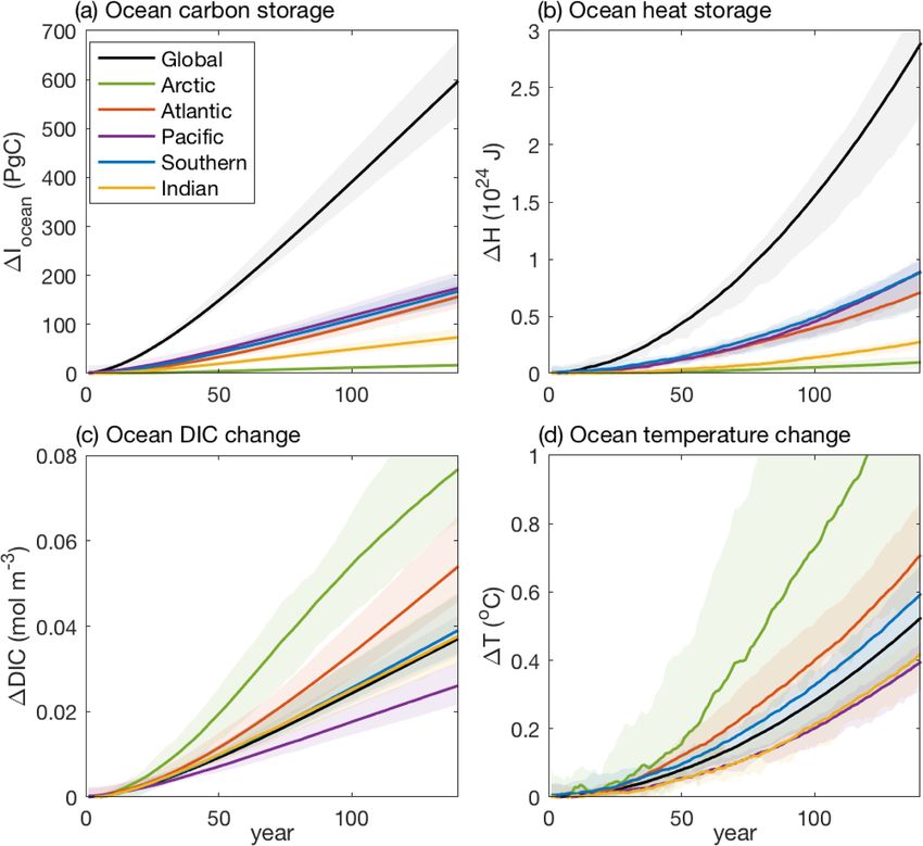
Figure 1. Carbon and heat storage for the global ocean and differ-
carbon–climate feedback is about 3 times stronger over the ent ocean basins in CMIP6 Earth system models: (a) ocean carbon
land than over the ocean on centennial timescales in the content changes relative to the pre-industrial in petagrams of car-
CMIP6 Earth system models (Arora et al., 2020). However, bon; (b) ocean heat content changes relative to the pre-industrial in
there is a substantial geographical variation in the ocean joules; (c) changes in the ocean dissolved inorganic carbon relative
carbon–climate feedback (Tjiputra et al., 2010; Roy et al., to the pre-industrial in moles per cubic metre, expressing the ocean
2011) as a result of an interplay between the effect of carbon- carbon storage changes per volume; and (d) changes in ocean tem-
ate chemistry, physical ventilation and biological processes. perature relative to the pre-industrial in degrees Celsius, expressing
In the tropics, the carbonate chemistry and the decrease in the ocean heat changes per volume. The solid lines show the model
solubility with warming drives a reduction in the ocean car- mean and the shading the model range based on the 1 % yr−1 in-
creasing CO2 experiment over 140 years in 11 CMIP6 models (Ta-
bon uptake with climate change (Roy et al., 2011; Rodgers
ble 1). For the definition of the ocean basins see Supplement Fig. S1.
et al., 2020). In the North Atlantic, the physical ventilation
and its weakening with warming acts to further reduce the
ocean carbon uptake with climate change (Yoshikawa et al.,
2008; Tjiputra et al., 2010; Roy et al., 2011). In the South- order asymmetry between the regional patterns of heat and
ern Ocean, changes in the cycling of biological material with carbon storage (Winton et al., 2013; Bronselaer and Zanna,
climate change can partly counteract the reduction in the 2020; Williams et al., 2021). The combined air–sea transfer
ocean carbon uptake due to the decrease in solubility and and transport effect leads to the Atlantic, Pacific and South-
physical ventilation with warming (Sarmiento et al., 1998; ern oceans each storing about 25 %–30 % of the additional
Bernardello et al., 2014). heat and carbon in CMIP6 models for a quadrupling of atmo-
The ocean carbon cycle feedbacks can be defined in terms spheric CO2 (Fig. 1a and b), despite their different sizes (see
of either the cumulative ocean carbon uptake or the ocean Supplement Fig. S1 for the basins’ definition). The Atlantic
carbon storage (Schwinger et al., 2014; Arora et al., 2020). and Arctic oceans have the largest increase in carbon and heat
For the global ocean, these two definition are almost equiv- per unit volume, as given by the dissolved inorganic carbon
alent apart from a small contribution from the land-to-ocean and temperature (Fig. 1c and d). The Pacific Ocean has the
carbon flux from river runoff and the carbon burial in ocean smallest increase in carbon and heat per unit volume (Fig. 1c
sediments (Arora et al., 2020). However, on a regional scale and d). Our motivation is to explore the mechanisms that lead
these two definitions are different, as the ocean carbon stor- to these regional variations in carbon storage and carbon cy-
age explicitly includes the convergence of transport of car- cle feedbacks in the different ocean basins in CMIP6 models.
bon by the ocean circulation. This transport effect leads to A mechanism that can affect the regional carbon storage
different geographical patterns for the ocean carbon storage is the Atlantic Meridional Overturning Circulation (AMOC).
and the ocean cumulative carbon uptake (Frölicher et al., The projected weakening in the AMOC with climate change
2015). This transport effect also leads to a broadly similar (Cheng et al., 2013) weakens the ocean physical ventilation
geographical distribution for ocean carbon and heat storage, and transport of carbon into the ocean interior, which acts to
with the “redistribution” of the pre-industrial carbon and heat reduce the ocean carbon uptake and storage (Sarmiento and
by changes in the circulation with warming driving a second- Le Quéré, 1996; Crueger et al., 2008). The weakening in the
Biogeosciences, 18, 3189–3218, 2021 https://doi.org/10.5194/bg-18-3189-2021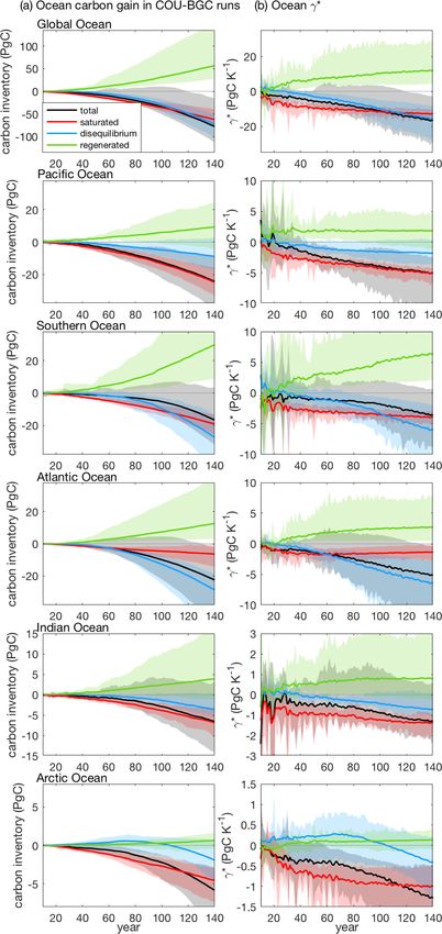
A. Katavouta and R. G. Williams: Ocean carbon cycle feedbacks in CMIP6 models                                                    3191

Table 1. List of the 11 CMIP6 Earth system models used in this    2     Ocean carbon cycle feedbacks in CMIP6 models
study along with references for the model description.
                                                                  2.1     Global ocean
         Earth system model    Reference
                                                                  In the carbon cycle feedback framework introduced by
         ACCESS-ESM1.5         Ziehn et al. (2020)                Friedlingstein et al. (2003, 2006) the ocean carbon gain due
         CanESM5               Swart et al. (2019g)
                                                                  to anthropogenic carbon emissions, 1Iocean , is expressed as
         CanESM5-CanOE         Swart et al. (2019g)
         CNRM-ESM2-1           Séférian et al. (2019)
                                                                  a function, F , of changes in the atmospheric CO2 and the
         GFDL-ESM4             Dunne et al. (2020)                physical climate:
         IPSL-CM6A-LR          Boucher et al. (2020)
         MIROC-ES2L            Hajima et al. (2020)
                                                                  1Iocean = F (CO2,0 + 1CO2 , T0 + 1T ) − F (CO2,0 , T0 ), (1)
         MPI-ESM1.2-LR         Mauritsen et al. (2019)
                                                                  where the surface air temperature, T , is used as a proxy
         MRI-ESM2              Yukimoto et al. (2019d)
         NorESM2-LM            Seland et al. (2020)
                                                                  for the physical climate and subscript 0 denotes the pre-
         UKESM1-0-LL           Sellar et al. (2019)               industrial state. By expanding the function F into a Taylor
                                                                  series (Schwinger et al., 2014; Williams et al., 2019), the
                                                                  ocean carbon gain relative to the pre-industrial era, 1Iocean ,
                                                                  is expressed as
AMOC with climate change also increases the residence time
in the ocean interior and the accumulation of remineralised                     ∂F           ∂F
carbon at depth, which acts to increase the ocean carbon up-      1Iocean =           1CO2 +                  1T
                                                                               ∂CO2 0        ∂T           0
take and storage (Sarmiento and Le Quéré, 1996; Joos et al.,
1999; Schwinger et al., 2014; Bernardello et al., 2014). Pre-                    ∂ 2F
                                                                           +                  1CO2 1T                             (2)
vious studies suggest that the combined effect of these two                    ∂CO2 ∂T    0
competing processes leads to a modest reduction in ocean                       ∂ 2F                 ∂ 2F
carbon uptake and storage with AMOC weakening and to an                    +             1CO22 +           1T 2 + R 3 ,           (3)
                                                                               ∂CO22 0              ∂T 2 0
ocean carbon–climate feedback that amplifies the increase in
atmospheric CO2 (Sarmiento and Le Quéré, 1996; Joos et al.,
                                                                  where R 3 contains the third-order and higher derivatives. By
1999; Crueger et al., 2008; Schwinger et al., 2014). However,
                                                                  ignoring the second- and higher-order terms but keeping the
the net effect of AMOC weakening with climate change on
                                                                  terms for the non-linear relationship between atmospheric
the carbon storage is highly uncertain and sensitive to the
                                                                  CO2 and climate change, Eq. (3) is rewritten as
representation of the vertical carbon gradient and ocean bi-
ological processes in Earth system models. This uncertainty       1Iocean = β1CO2 + γ 1T + N 1CO2 1T ,                            (4)
motivates us to explore the control of the AMOC on the car-
bon cycle feedbacks in CMIP6 models, as well as the relative      where the ocean carbon–concentration feedback parameter is
importance of changes in biological processes and physical                         ∂F
                                                                  defined as β = ∂CO    , the ocean carbon–climate feedback
                                                                                      2    0
ventilation for the carbon storage in different ocean basins.                                      ∂F
   Our aim is to provide insight into the relative contribution   parameter is defined as γ =      ∂T 0   and the non-linearity of the
                                                                                                                         ∂ F 2
of different ocean basins to the ocean carbon cycle feedbacks     ocean carbon cycle feedbacks is defined as N = ∂CO              .
                                                                                                                           2 ∂T 0
and the processes that drive this regional partitioning in the       The carbon cycle feedback parameters, β and γ , are tra-
CMIP6 models. In Sect. 2, we provide the framework for            ditionally estimated using Earth system model simulations
the carbon cycle feedbacks and explore their geographical         with the couplings between the carbon cycle and radiative
distribution in 11 CMIP6 Earth system models (Table 1). In        forcing switched either on or off: a fully coupled simula-
Sect. 3, the ocean carbon cycle feedbacks are separated into      tion, a radiatively coupled simulation and a biogeochemi-
contribution from carbonate chemistry, physical ventilation       cally coupled simulation (Friedlingstein et al., 2006; Arora
and biological processes, and the controls of the global and      et al., 2013; Jones et al., 2016; Arora et al., 2020). Any com-
regional feedbacks are investigated in diagnostics of CMIP6       bination of these three simulations can be used to estimate the
models. In Sect. 4, the effect of the AMOC on the global          carbon cycle feedback parameters; however, each combina-
and basin-scale carbon cycle feedbacks is investigated, firstly   tion yields somewhat different results due to the non-linearity
using an idealised climate model that provides a mechanistic      of the system (Gregory et al., 2009; Zickfeld et al., 2011;
insight and then in diagnostics of CMIP6 models. Section 5        Schwinger et al., 2014; Arora et al., 2020). Here, we esti-
summarises our conclusions and discusses the wider context        mate the carbon cycle feedback parameters using the fully
of our analysis.                                                  coupled simulation (COU) and the biogeochemically cou-
                                                                  pled simulation (BGC) under the 1 % yr−1 increasing CO2
                                                                  experiment, in which the atmospheric CO2 concentration in-
                                                                  creases from its pre-industrial value of around 285 ppm until

https://doi.org/10.5194/bg-18-3189-2021                                                       Biogeosciences, 18, 3189–3218, 2021
3192                                                   A. Katavouta and R. G. Williams: Ocean carbon cycle feedbacks in CMIP6 models

it quadruples over a 140-year period, following the recom-                        cycle feedback parameters for each ocean region n are ex-
mended C4 MIP protocol of experiments (Jones et al., 2016;                        pressed as
Arora et al., 2020). To remove the effect of model drift and
reduce model biases, the pre-industrial control simulation                                1SnBGC
                                                                                  βn =           ,
(piControl) was used to estimate the pre-industrial state in                              1CO2
the Earth system models. For simplicity, we ignore the effect                             1SnCOU − 1SnBGC
of the air temperature increase in the BGC simulation on the                      γn =                    ,                                  (7)
                                                                                                1T
feedbacks, which has a contribution of less than 5 % (Arora
et al., 2020), such that                                                          where the carbon–climate feedback parameter, γn , corre-
                                                                                  sponds to the effect of climate change under rising at-
        BGC
      1Iocean                                                                     mospheric CO2 and hence includes the effect of the non-
β=            ,                                                                   linearity, Nn 1CO2 , in Eq. (6).
      1CO2
         COU − 1I BGC                                                                Alternatively, the carbon cycle feedbacks can be defined
       1Iocean   ocean
γ=                     ,                                                    (5)   based on the carbon storage, such that the regional carbon
              1T                                                                  cycle feedback parameters for each ocean region n are ex-
where 1CO2 is the increase in atmospheric CO2 and 1T                              pressed as
is the increase in air surface temperature in the fully cou-
                                                                                          1InBGC
pled Earth system (i.e. COU simulation) relative to the pre-                      βn∗ =          ,
industrial state. The carbon–climate feedback parameter, γ ,                              1CO2
in Eq. (5) corresponds to the effect of climate change under                              1InCOU − 1InBGC
                                                                                  γn∗ =                   ,                                  (8)
rising atmospheric CO2 and hence includes the effect of the                                     1T
non-linearity, N 1CO2 , in Eq. (4) (Schwinger et al., 2014).
                                                                                  where 1In is the change in the carbon inventory in region
   The ocean carbon–concentration feedback parameter, β,
                                                                                  n. The carbon storage includes the combined effect from the
is positive in all the CMIP6 models (Table 2). The ocean
                                                                                  local air–sea carbon exchange and the transport of carbon by
carbon–climate feedback parameter, γ , is negative in all the
                                                                                  the ocean circulation, such that
Earth system models (Table 2), indicating that the ocean
takes up less carbon in response to climate change. The vari-                     1In = 1Sn + 1Gn ,                                          (9)
ability in β amongst the Earth system models, as described
by the coefficient of variation, CV, is relatively small on                       where 1Sn is the regional cumulative ocean carbon uptake
the global scale (CV = 0.09) when compared with the vari-                         from the atmosphere relative to the pre-industrial era, and
ability in γ (CV = 0.43) (Table 2). However, for the uncer-                       1Gn is the regional cumulative carbon gain relative to the
tainty in the ocean carbon gain due to carbon emissions,                          pre-industrial era due to the ocean transport.
the carbon–concentration feedback contributes to a spread of                         By substituting Eqs. (9) and (7) in Eq. (8) the two defi-
62 PgC, while the carbon–climate feedback contributes only                        nitions for the carbon cycle feedback parameters are related
to a spread of 25 PgC amongst the CMIP6 Earth system mod-                         by
els on a global scale and to a quadrupling of atmospheric
CO2 , where the spread corresponds to 1 standard deviation.                                 1GnBGC
                                                                                  βn∗ = βn +       ,
                                                                                             1CO2
2.2    Regional ocean
                                                                                              1GnCOU − 1GnBGC

                                                                                   ∗
                                                                                  γn = γn +                     .                          (10)
The carbon cycle feedbacks for the global ocean in Eq. (4)                                           1T
can be further separated into contributions from different                        Eq. (10) shows that the feedback parameters defined by the
ocean regions such that                                                           regional carbon storage, β ∗ and γ ∗ , are proportional to the
            global               global             global
                                                                                  feedback parameters defined by the regional cumulative car-
                                                                                  bon uptake, γ and β, but further modified by the ocean car-
             X                    X                  X
1Iocean =            βn 1CO2 +            γn 1T +            Nn 1CO2 1T ,   (6)
            n=1                  n=1                n=1                           bon transport.
where n denotes the different ocean regions; 1CO2 and 1T                          2.2.1    Estimates based on carbon storage versus carbon
are the global changes in atmospheric CO2 and the surface air                              uptake
temperature, respectively; and βn , γn and Nn are the carbon
cycle feedback parameters and their non-linearity for each                        On a global scale, the
                                                                                                      P transport effect on the carbon storage
ocean region n.                                                                   integrates to zero, global
                                                                                                         n    1Gn = 0, such that the feedback
   Traditionally, the carbon cycle feedbacks are defined based                    parameters estimated from the carbon storage, β ∗ and γ ∗ ,
on the cumulative carbon uptake from the atmosphere, 1S                           are equivalent to the feedback parameters estimated from the
(Tjiputra et al., 2010; Roy et al., 2011) such that the carbon                    cumulative carbon uptake, β and γ , when ignoring the small

Biogeosciences, 18, 3189–3218, 2021                                                                  https://doi.org/10.5194/bg-18-3189-2021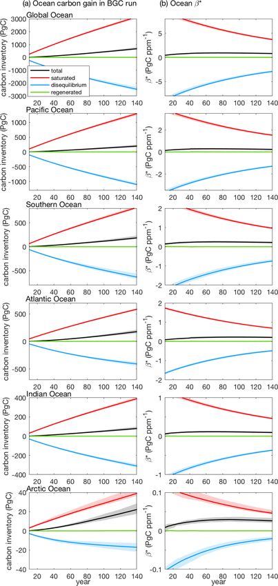
A. Katavouta and R. G. Williams: Ocean carbon cycle feedbacks in CMIP6 models                                                        3193

Table 2. Carbon–concentration feedback parameter based on carbon storage, β ∗ (PgC ppm−1 ), and carbon–climate feedback parameter based
on carbon storage, γ ∗ (PgC K−1 ), for the global ocean and different ocean basins in 11 CMIP6 Earth system models, along with the inter-
model mean; standard deviation; and coefficient of variation (CV), estimated as the standard deviation divided by the mean. The estimates
are based on the fully coupled simulation (COU) and the biogeochemically coupled simulation (BGC) under the 1 % yr−1 increasing CO2
experiment. Diagnostics are from years 121 to 140 (the 20 years up to quadrupling of atmospheric CO2 ). Note that for the global ocean, β ∗
and γ ∗ are equivalent to β and γ .

                         Parameter β ∗
                         Model                Global ocean      Pacific    Southern    Atlantic   Indian   Arctic
                         ACCESS-ESM1.5                0.901      0.247         0.277     0.241     0.099    0.029
                         CanESM5                      0.794      0.256         0.210     0.192     0.098    0.027
                         CanESM5-CanOE                0.750      0.241         0.202     0.178     0.094    0.024
                         CNRM-ESM2-1                  0.794      0.251         0.191     0.210     0.103    0.027
                         GFDL-ESM4                    0.933      0.278         0.250     0.257     0.107    0.028
                         IPSL-CM6A-LR                 0.777      0.249         0.201     0.192     0.101    0.023
                         MIROC-ES2L                   0.762      0.220         0.214     0.196     0.083    0.034
                         MPI-ESM1.2-LR                0.803      0.237         0.235     0.211     0.085    0.022
                         MRI-ESM2                     0.966      0.306         0.235     0.258     0.121    0.030
                         NorESM2-LM                   0.815      0.197         0.252     0.236     0.088    0.024
                         UKESM1-0-LL                  0.736      0.198         0.192     0.203     0.102    0.029
                         Mean                         0.821      0.244         0.224     0.216     0.098    0.027
                         SD                           0.077      0.032         0.028     0.028     0.011    0.004
                         CV                           0.094      0.131         0.125     0.130     0.112    0.148
                         Parameter γ ∗
                         Model                Global ocean      Pacific    Southern    Atlantic   Indian   Arctic
                         ACCESS-ESM1.5              −20.56      −8.79         −6.40     −3.34     −1.15    −0.64
                         CanESM5                    −13.94      −5.41         −2.59     −2.65     −1.94    −0.87
                         CanESM5-CanOE              −11.21      −4.40         −2.22     −2.16     −1.26    −0.72
                         CNRM-ESM2-1                 −1.54      −2.16          0.90     −0.04      0.61    −0.61
                         GFDL-ESM4                  −18.41      −5.70         −2.58     −6.35     −2.06    −1.69
                         IPSL-CM6A-LR               −11.82      −4.76         −2.28     −3.07     −1.03    −0.48
                         MIROC-ES2L                 −19.08      −3.06         −4.35     −7.40     −1.84    −2.54
                         MPI-ESM1.2-LR              −16.70      −2.77         −5.39     −5.99     −1.19    −0.81
                         MRI-ESM2                   −27.64     −10.42          0.19    −12.19     −1.64    −2.61
                         NorESM2-LM                 −18.00      −2.43         −8.35     −6.13     −0.13    −0.87
                         UKESM1-0-LL                −11.94      −2.84         −2.23     −3.28     −2.05    −1.02
                         Mean                       −15.53      −4.80         −3.21     −4.78     −1.24    −1.17
                         SD                           6.66       2.69          2.73      3.30      0.84     0.76
                         CV                           0.43       0.56          0.85      0.69      0.68     0.65

carbon exchange between land and ocean. However, on re-                   cal gyres, the ocean anthropogenic carbon uptake is limited
gional scales the effect of the ocean transport on carbon stor-           and β is small (Fig. 2b).
age leads to different spatial patterns in these carbon cycle                The carbon–concentration feedback parameter estimated
feedback parameters, β and β ∗ and γ and γ ∗ (Fig. 2).                    from ocean carbon storage, β ∗ , is again large in the North
   The carbon–concentration feedback parameter estimated                  Atlantic but instead large in the Southern Hemisphere sub-
from the cumulative carbon uptake, β, is largest and has more             tropical gyres and small in the Southern Ocean south of 50◦ S
inter-model variability in (i) the Southern Ocean, (ii) the east-         relative to β (Fig. 2a). This difference between β and β ∗
ern boundary upwelling regions, (iii) the Gulf Stream and                 (Supplement Fig. S2) is due to the northward transport of
its extension into the North Atlantic Current, and (iv) the               anthropogenic carbon from the Southern Ocean associated
Kuroshio Extension (Fig. 2b). The inter-model variability                 with subduction and transport of mode and intermediate wa-
in β is also significant along the equatorial Pacific, with               ters. The variability in β ∗ amongst the models is large in the
this variability related to the inter-model spread in the trade           North Atlantic and extends south along the Atlantic western
winds and equatorial upwelling. In contrast, in the subtropi-             boundary (Fig. 2a).

https://doi.org/10.5194/bg-18-3189-2021                                                           Biogeosciences, 18, 3189–3218, 2021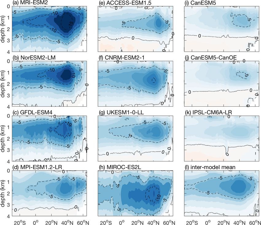
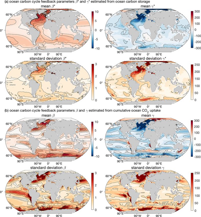
3194                                    A. Katavouta and R. G. Williams: Ocean carbon cycle feedbacks in CMIP6 models

Figure 2. Geographical distribution of the carbon cycle feedback parameters normalised by area: (a) β ∗ (gC ppm−1 m−2 ) and γ ∗
(gC K−1 m−2 ), estimated based on the regional ocean carbon storage, and (b) β (gC ppm−1 m−2 ) and γ (gC K−1 m−2 ), estimated based
on the regional cumulative ocean carbon uptake. Results are shown as the inter-model mean and standard deviation based on 11 CMIP6
Earth system models (Table 1). The estimates are based on the fully coupled simulation (COU) and the biogeochemically coupled simulation
(BGC) under the 1 % yr−1 increasing CO2 experiment. Diagnostics are from years 121 to 140 (the 20 years up to quadrupling of atmospheric
CO2 ).

   The carbon–climate feedback parameter estimated from               γ ∗ that is overall less negative in the Southern Ocean and
the cumulative carbon uptake, γ , is large and negative in the        in the high latitudes of the North Atlantic but more negative
North Atlantic and in the Southern Ocean from 50 to 65◦ S             in the Arctic, the equatorial Pacific and along the Atlantic
(Fig. 2b). In contrast, γ is large and positive in a narrow band      western boundary relative to γ (Fig. 2a). The spread in γ ∗
between 40 and 45◦ S, in the Southern Hemisphere eastern              amongst the models is largest in the North Atlantic, in the
boundary upwelling regions, and in polar regions with sea             Arctic, along the Atlantic western boundary and in the South-
ice. The regions of large ocean carbon loss or uptake from            ern Ocean (Fig. 2a).
the atmosphere due to climate change, as shown by the large              The carbon cycle feedbacks estimated from the cumulative
γ , also experience the largest variability in γ amongst the          carbon uptake better describe the atmosphere–ocean interac-
CMIP6 Earth system models (Fig. 2b).                                  tion. The carbon cycle feedbacks estimated from the ocean
   The effect of carbon transport on γ ∗ is of opposite sign          carbon storage instead better describe the response of the
to the effect of the cumulative carbon uptake in most re-             ocean carbon budget to carbon emissions. Here, we focus
gions (Supplement Fig. S2). This transport effect leads to a          on the carbon cycle feedbacks estimated from the regional

Biogeosciences, 18, 3189–3218, 2021                                                       https://doi.org/10.5194/bg-18-3189-2021
A. Katavouta and R. G. Williams: Ocean carbon cycle feedbacks in CMIP6 models                                               3195

ocean carbon storage to enable diagnostics in terms of the        carbon pools: (i) the DICsat representing the amount of DIC
preformed and regenerated carbon pools and to gain more           that the ocean would have if the whole ocean reached a full
mechanistic insight.                                              chemical equilibrium with the contemporaneous atmospheric
                                                                  CO2 concentration and (ii) the DICdis representing the ex-
2.2.2   Basin-scale β ∗ and γ ∗                                   tent that the ocean departs from a full chemical equilibrium
                                                                  with the contemporaneous atmospheric CO2 . Assuming the
We define the Southern Ocean as south of 35◦ S and the            changes in the biological organic carbon inventory are small,
Arctic Ocean as north of 65◦ N, and we exclude semi-              the changes in the ocean carbon inventory relative to the pre-
enclosed seas from our basins’ definition (see Supplement         industrial era, 1Iocean in petagrams of carbon, are related to
Fig. S1 for a map of the regions). The Pacific, Southern          the volume integral of the changes in each of the DIC pools,
and Atlantic oceans contribute equally to the ocean carbon–       1DIC in moles per cubic metre, as
concentration feedback parameter, as estimated in terms                         Z
of carbon storage, with an inter-model mean β ∗ of 0.24,          1Iocean = m      1DICsat + 1DICdis + 1DICreg dV

0.22 and 0.22 PgC ppm−1 , respectively (Table 2). The Indian
                                                                                  V
Ocean contributes less than half than the other three basins to
β ∗ , with an inter-model mean of 0.10 PgC ppm−1 (Table 2).                = 1Isat + 1Idis + 1Ireg ,                         (12)
The Arctic Ocean has a β ∗ of only 0.03 PgC ppm−1 . The Pa-       where m = 12.01 × 10⁻¹⁵ PgC mol−1 is a unit conversion
cific, Southern, Atlantic, Indian and Arctic oceans have an       from moles to petagrams of carbon.
inter-model mean carbon–climate feedback parameter, de-              By substituting Eq. (12) into Eq. (5), for the global ocean,
fined in terms of carbon storage, γ ∗ , of −4.8, −3.2, −4.8,      or into Eq. (8), for the regional ocean, the carbon cycle feed-
−1.2 and −1.2 PgC K−1 , respectively (Table 2). The basin-        back parameters may be diagnosed in terms of these differ-
scale variability in β ∗ amongst the models, as described by      ent ocean carbon pools (Williams et al., 2019; Arora et al.,
the coefficient of variation, CV, is less than 0.15 (Table 2).    2020):
The basin-scale variability in γ ∗ amongst the models varies
                                                                                                 BGC     BGC     BGC
                                                                                                               1Ireg
from CV = 0.56 in the Pacific Ocean to CV = 0.85 in the                                        1Isat   1Idis
                                                                  β ∗ = βsat + βdis + βreg =         +       +       ,
Southern Ocean (Table 2). The inter-model variability in β ∗                                   1CO2    1CO2    1CO2
and γ ∗ for each basin is larger than that of the global ocean                             COU − 1I BGC
                                                                                        1Isat       sat
(Table 2), which suggests that variability in different basins    γ ∗ = γsat + γdis + γreg =
                                                                                              1T
compensate for each other. For diagnostics of the separate                COU − 1I BGC       COU − 1I BGC
                                                                       1Idis             1Ireg        reg
contribution of the ocean carbon uptake and transport on the         +            dis
                                                                                       +                  .         (13)
basin-scale carbon storage and for feedback parameters see                     1T               1T
Appendix A.                                                       3.1 Contribution from the saturated carbon pool to β ∗
                                                                       and γ ∗
3   Processes controlling the carbon cycle feedbacks in           The saturated part of β ∗ and γ ∗ in Eq. (13) is expressed as
    CMIP6 models                                                             BGC
                                                                           1Isat
                                                                  βsat =         ,
To gain insight into the driving mechanisms of the carbon                  1CO2
cycle feedbacks and their uncertainty amongst Earth system                   COU − 1I BGC
                                                                         1Isat          sat
models, β ∗ and γ ∗ may be separated into contribution from       γsat =                    ,                              (14)
                                                                                 1T
the regenerated, the saturated and the disequilibrium ocean
carbon pools following the methodology of Williams et al.         The changes in the saturated carbon pool relative to the pre-
(2019) and Arora et al. (2020). The ocean dissolved inor-         industrial era in Eq. (14) are diagnosed as
                                                                             Z
ganic carbon, DIC, may be defined in terms of these separate
                                                                  1Isat = m 1DICsat dV
carbon pools (Ito and Follows, 2005; Williams and Follows,
2011; Lauderdale et al., 2013; Bernardello et al., 2014):                     V
                                                                           Z

DIC = DICpref + DICreg = DICsat + DICdis + DICreg , (11)                = m 1f CO2 , Tocean , S, P , Si, Alkpre dV ,         (15)
where DICpref is the part of the DIC transferred from the sur-                V
face into the ocean interior due to the physical ventilation,     where 1 is the change relative to the pre-industrial era, Tocean
involving the circulation, and DICreg is the part of the DIC      is the ocean temperature, S is the ocean salinity, P is the
accumulated into the ocean interior due to biological regener-    ocean phosphate concentration, Si is the ocean silicate con-
ation of organic carbon. Similarly, the DICpre can be viewed      centration, Alkpre is the preformed alkalinity and f is a non-
as the part of the DIC associated with the solubility pump and    linear function representing the solution to the ocean car-
the DICreg as the part of the DIC associated with the biologi-    bonate chemistry which provides DICsat for the contempo-
cal pump. The DICpref can be further split into two idealised     raneous atmospheric CO2 . Here, f is estimated following

https://doi.org/10.5194/bg-18-3189-2021                                                   Biogeosciences, 18, 3189–3218, 2021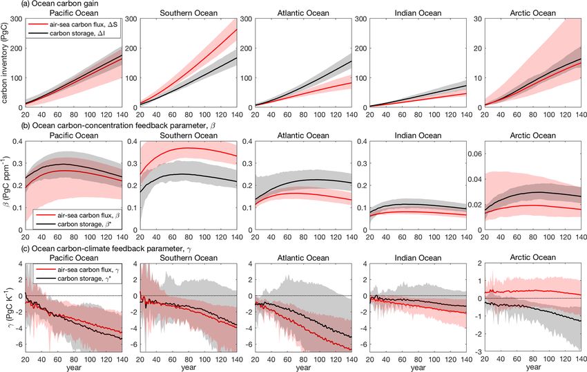
3196                                        A. Katavouta and R. G. Williams: Ocean carbon cycle feedbacks in CMIP6 models

the iterative solution for the ocean carbonate chemistry of
Follows et al. (2006) and by considering the small contri-
bution of minor species (borate, phosphate, silicate) to the
preformed alkalinity. In the limit that the ocean hydrogen ion
concentration at a chemical equilibrium with the given atmo-
spheric CO2 , [H+ ]sat , is known or the preformed alkalinity
is assumed equal to the carbonate alkalinity, the f function
corresponds to the usual solution of the carbonate system that
provides DICsat based on two knowns: atmospheric CO2 and
either [H+ ]sat (see Eq. 18) or carbonate alkalinity. The pre-
formed alkalinity is estimated from a multiple linear regres-
sion using salinity and the conservative tracer PO (Gruber
et al., 1996), with the coefficients of this regression estimated
based on the surface (first 10 m) alkalinity, salinity, oxygen
and phosphate in each of the Earth system models.
   To understand how the ocean carbonate chemistry oper-
ates and the mechanisms that control βsat , consider an ocean
buffer factor, B, where the fractional change in the atmo-
spheric CO2 and saturated carbon inventory is defined rela-
tive to the pre-industrial era (Katavouta et al., 2018):
       1CO2 /CO2,0
B=                    ,                                       (16)
        1Isat /Isat,0

where subscript 0 denotes the pre-industrial era.
  Substituting Eq. (16) into Eq. (14) the saturated part of β ∗
can be expressed as
                          1                 Isat,0
βsat =                                             ,          (17)
         B(CO2 , Tocean,0 , S0 , Alkpre,0 ) CO2,0

where B(CO2 , Tocean,0 , S0 , Alk0 ) is the ocean buffer factor
for the increasing atmospheric CO2 but with no climate
change (i.e. for the pre-industrial ocean temperature, salin-
ity and alkalinity), as is the case in the BGC run.
   Eq. (17) shows that βsat is proportional to the ocean capac-
ity to buffer changes in atmospheric CO2 with no changes
in the physical climate, B(CO2 , Tocean,0 , S0 , Alkpre,0 )−1 . The
rise in atmospheric CO2 leads not only to an increase in the
saturated ocean carbon inventory, 1Isat (Fig. 3a, red shade),
but also to a decrease in the ocean capacity to buffer changes
in atmospheric CO2 as the ocean acidifies. Accordingly, the
buffer factor, B, increases and βsat decreases with the rise in
atmospheric CO2 at a global and basin scale in all the Earth
system models (Fig. 3b, red shade). The buffer factor, B, and
thus βsat also depend on the pre-industrial ocean state due           Figure 3. Ocean carbon storage and ocean carbon–concentration
to the non-linearity of the ocean carbonate system. Hence,            feedback parameter, β ∗ , for the global ocean and different ocean
there is a spread in βsat amongst the Earth system models             basins, along with the contribution from the saturated, disequilib-
forced by the same increase in atmospheric CO2 (Fig. 3b,              rium and regenerated carbon pools in CMIP6 Earth system models:
                                                                      (a) ocean carbon inventory changes relative to the pre-industrial era
red shade) related to their different pre-industrial ocean tem-
                                                                      in the biogeochemically coupled simulation (BGC) and (b) ocean
perature, salinity and alkalinity.
                                                                      carbon–concentration feedback parameter based on carbon storage,
   To understand the mechanisms that control γsat , consider          β ∗ (PgC ppm−1 ). The solid lines and the shading show the model
the solution to the saturated part of DIC as dictated by the          mean and the model range, respectively, based on the 1 % yr−1 in-
carbonate chemistry,                                                  creasing CO2 experiment over 140 years in 11 CMIP6 models (Ta-
                                                                      ble 1). Note that for the global ocean, β ∗ is equivalent to β.
                                     2−
DICsat = [CO2 ]sat + [HCO−
                         3 ]sat + [CO3 ]sat

Biogeosciences, 18, 3189–3218, 2021                                                       https://doi.org/10.5194/bg-18-3189-2021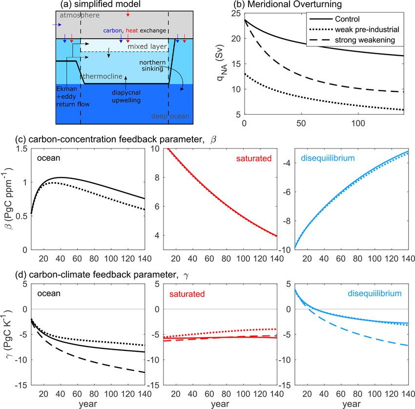
A. Katavouta and R. G. Williams: Ocean carbon cycle feedbacks in CMIP6 models 3197
Ko K1 Ko K1 K2 consistent with the carbonate system being less sensitive to
= CO2 Ko + + + , (18)
[H ]sat [H+ ]2sat change in temperature under higher ocean DIC (Schwinger
et al., 2014).
where Eq. (20) shows that γsat is proportional to the changes
in solubility due to climate change and is further modified
[CO2 ]sat is Ko CO2 ,
by changes in the ocean carbon dissociation constants with
K1 warming and by the non-linearity of the carbonate chemistry.
[HCO− ]
3 sat is CO K
2 o ,
[H+ ]sat Ocean warming due to climate change leads to a decrease in
2− K1 K2 the saturated carbon inventory, 1Isat , in all basins (Fig. 4a,
[CO3 ]sat is CO2 Ko ,
[H+ ]2sat red shade) primarily driven by a decrease in solubility. This
decrease in 1Isat with warming drives a nearly constant neg-
Ko is the solubility, K1 and K2 are the ocean carbon dissocia- ative γsat (Fig. 4b, red shade) with the deviations from a con-
tion constants, and [H+ ]sat is the ocean hydrogen ion concen- stant value being associated with the non-linearity of the car-
tration at a chemical equilibrium with the contemporaneous bonate system. The spread of γsat amongst the Earth system
atmospheric CO2 . Ko , K1 and K2 are a function of the ocean models (Fig. 4b, red shade) is relatively small at a global and
temperature and salinity and so depend on the physical cli- basin scale, except in the Arctic, and is associated with dif-
mate change, while [H+ ]sat depends primarily on the changes ferent pre-industrial ocean states in the models.
in atmospheric CO2 . Combining Eq. (18) with Eqs. (14) and
(15) and assuming that the ocean temperature and salinity 3.2 Contribution from the regenerated carbon pool to
remain at their pre-industrial value in the BGC run with no β ∗ and γ ∗
climate change, γsat can be expressed as
Z The regenerated part of β ∗ and γ ∗ in Eq. (13) is expressed as
m 1 (Ko K1 ) 1 (Ko K1 K2 )
γsat = CO2 1Ko + + dV . (19) BGC
1T [H+ ]sat [H+ ]2sat 1Ireg
V βreg = ,
1CO2
By expanding [H+ ]sat = [H+ ]sat,0 +1[H+ ]sat , Eq. (19) can COU − 1I BGC
1Ireg reg
be written as γreg = . (21)
1T
Z ( ) Assuming that the oxygen concentration is close to satura-
m 1 (Ko K1 ) 1 (Ko K1 K2 )
γsat = CO2 1Ko +
+ tion at the surface, DICreg can be estimated from the appar-
1T [H+ ]0,sat [H+ ]20,sat
V | {z } ent oxygen utilisation, AOU, and the contribution of biolog-
effect of ocean warming under pH0
ical calcification to alkalinity, Alk (Ito and Follows, 2005;
Williams and Follows, 2011; Lauderdale et al., 2013), such
)
that 1Ireg in Eq. (21) is diagnosed as
(
1 (Ko K1 ) 1[H+ ]sat 1 (Ko K1 K2 ) 1 [H+ ]2sat
− + dV .
(20)
[H+ ]0,sat [H+ ]sat [H + ]20,sat [H+ ]2sat
| {z } Z Z
effect of ocean warming under 1pH 1Ireg = m 1DICreg dV = m RCO 1AOU
The first term in curly brackets in Eq. (20) contributes V V
to the linear part of γsat and is controlled by changes in 1
climate only, specifically by the effect of changes in the + 1Alk − 1Alkpre − RNO 1AOU dV , (22)
2
ocean temperature to the solubility and ocean carbon dis-
sociation constants. Under warming due to changes in cli- where RCO and RNO are constant stoichiometric ratios and
mate, this term is negative. The second term in curly brack- Alkpre is the preformed alkalinity such that Alk−Alkpre gives
ets in Eq. (20) contributes to the non-linear part of γsat , and the contribution to alkalinity from biological calcification.
it depends on changes in pH, due to the increase in atmo- The regenerated part of β ∗ is associated with changes in
spheric CO2 , and changes in climate. Under rising atmo- ocean biological processes due to the atmospheric CO2 in-
spheric CO2 and warming, this term is negative as [H+ ]sat BGC and β
crease. 1Ireg reg are effectively negligible in the Earth
increases and+]
Ko decreases, and it is smaller than the linear system models (Fig. 3a and b, green shade) as these mod-
term as 1[H sat
[H+ ]sat
< 1. The adjustment of γsat due to changes els do not include an explicit dependence of biological pro-
in the pH, represented by this non-linear term, depends on duction on an increase in carbon availability or decrease in
the increase in atmospheric CO2 ; for example, the non-linear seawater pH. The regenerated part of γ ∗ is associated with
term is about 30 % and 50 % of the linear term for a doubling changes in ocean biological processes due to changes in cli-
of atmospheric CO2 and for a quadrupling of atmospheric mate, including the effect of changes in the circulation on the
CO2 , respectively. Hence, the non-linearity of the carbonate sinking rate of particles, the effect of warming on the solu-
chemistry acts to reduce the magnitude of the negative γsat bility of oxygen and the effect of changes in alkalinity on
https://doi.org/10.5194/bg-18-3189-2021 Biogeosciences, 18, 3189–3218, 2021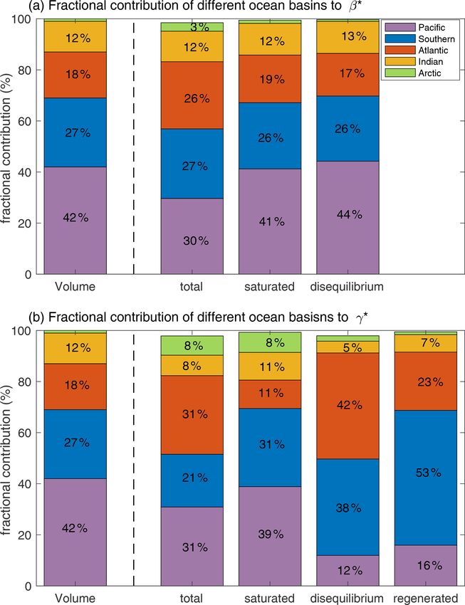
3198                                     A. Katavouta and R. G. Williams: Ocean carbon cycle feedbacks in CMIP6 models

                                                                      the dissolution of the calcium carbonate shells of calcifying
                                                                      phytoplankton. 1IregCOU − 1I BGC and γ
                                                                                                    reg         reg are positive and
                                                                      increase in time on a global and basin scale (Fig. 4a and b,
                                                                      green shade), indicating that γreg is dominated by the weak-
                                                                      ening in the ocean physical ventilation due to climate change.
                                                                      This weakening in the ocean physical ventilation leads to a
                                                                      longer residence time of water masses in the ocean interior
                                                                      and so to an increase in the accumulation of carbon from the
                                                                      regeneration of biologically cycled carbon in the deep ocean
                                                                      (Schwinger et al., 2014; Bernardello et al., 2014).

                                                                      3.3   Contribution from the disequilibrium carbon pool
                                                                            to β ∗ and γ ∗

                                                                      The disequilibrium parts of β ∗ and γ ∗ are diagnosed using
                                                                      Eq. (13) as
                                                                      βdis = β ∗ − βsat − βreg ,
                                                                      γdis = γ ∗ − γsat − γreg .                                  (23)
                                                                         The disequilibrium part of the carbon cycle feedback pa-
                                                                      rameters is controlled by the ocean physical ventilation.
                                                                      Specifically, βdis is a function of the pre-industrial ocean
                                                                      physical ventilation and the rate of transfer of the anthro-
                                                                      pogenic carbon from the ocean surface into the ocean in-
                                                                      terior. The rise in atmospheric CO2 leads to an increase in
                                                                      the magnitude of the negative disequilibrium ocean carbon
                                                                      inventory, 1Idis , at a global and basin scale (Fig. 3a, blue
                                                                      shade), as the ocean physical ventilation is relatively slow
                                                                      and the ocean carbon transfer over the ocean interior cannot
                                                                      keep up with the rate of increase in atmospheric CO2 . Hence,
                                                                      βdis is negative at a global and basin scale in all the Earth
                                                                      system models (Fig. 3b, blue shade). However, the rate of in-
                                                                      crease in the magnitude of 1Idis slows down in time (Fig. 3a,
                                                                      blue shade) and βdis becomes less negative in time (Fig. 3b,
                                                                      blue shade), as more anthropogenic carbon is transferred into
                                                                      the ocean interior while the buffer capacity of the ocean de-
                                                                      creases, which brings the ocean closer to an equilibrium with
                                                                      the contemporaneous atmospheric CO2 .
                                                                         The disequilibrium part of γ ∗ depends on the weakening
                                                                      of the ocean physical ventilation with climate change. Here,
                                                                      γdis is defined based on the climate change impact under ris-
                                                                      ing atmospheric CO2 (i.e. COU–BGC runs) and so includes
                                                                      (i) the effect of weakening ventilation on the pre-industrial
                                                                      ocean carbon gradient involving the natural carbon, (ii) the
Figure 4. Ocean carbon storage and ocean carbon–climate feed-         effect of weakening ventilation on the anthropogenic carbon,
back parameter, γ ∗ , for the global ocean and different ocean        and (iii) the effect from decreasing sea-ice coverage leading
basins, along with the contribution from the saturated, disequilib-   to an increase in the ocean in direct contact with the atmo-
rium and regenerated carbon pools in CMIP6 Earth system models:       sphere. Overall, the effect of the weakening ventilation on
(a) ocean carbon inventory changes in the fully coupled simulation    the combined anthropogenic and natural carbon leads to a
(COU) minus the biogeochemically coupled simulation (BGC) and         negative 1Idis and a negative γdis on a global scale and in the
(b) ocean carbon–climate feedback parameter based on carbon stor-
                                                                      Atlantic, Indian, Pacific and Southern oceans after year 40
age, γ ∗ (PgC K−1 ). The solid lines and the shading show the model
                                                                      (Fig. 4a and b, blue shade). In the Arctic, the effect of the de-
mean and the model range, respectively, based on the 1 % yr−1 in-
creasing CO2 experiment over 140 years in 11 CMIP6 models (Ta-        creasing sea-ice coverage drives a slightly positive γdis over
ble 1). Note that for the global ocean, γ ∗ is equivalent to γ .      the first 80 years, while the effect of the weakening ventila-
                                                                      tion dominates and drives a negative γdis after year 80. The

Biogeosciences, 18, 3189–3218, 2021                                                       https://doi.org/10.5194/bg-18-3189-2021
A. Katavouta and R. G. Williams: Ocean carbon cycle feedbacks in CMIP6 models 3199
disequilibrium part of γ ∗ becomes more negative in time on a quilibrium carbon pool (Fig. 5b, red circles) and the reduc-
global and basin scale as the ocean ventilation weakens with tion in the physical ventilation due to climate change, with
warming. the contribution from the saturated carbon pool being rela-
tively small. In the Arctic Ocean, γ ∗ is primarily controlled
3.4 Combined effect of saturated, disequilibrium and by the saturated carbon pool and the decrease in solubility,
regenerated carbon pools on β ∗ and γ ∗ with the contribution from the regenerated carbon pool being
negligible (Fig. 5b, green circles).
On a global and basin scale, the ocean carbon–concentration On regional scales, the contributions from the saturated,
feedback parameter, β ∗ , is positive in all the Earth system disequilibrium and regenerated carbon pools to β ∗ and γ ∗
models. This positive β ∗ is explained by the chemical re- are further modified by local upwelling, changes in alkalinity
sponse involving the rise in ocean saturation, βsat , opposed and the conversion of regenerated carbon to disequilibrium
by the effect of the relatively slow ocean ventilation, such carbon at the ocean surface, as discussed in Appendix B.
that the physical uptake of carbon within the ocean is unable
to keep pace with the rise in atmospheric CO2 , βdis (Fig. 3b). 3.5 Processes controlling the contribution from
There is no significant contribution from biological changes different basins to β ∗ and γ ∗
to β ∗ in the Earth system models. The spread in βsat amongst
the Earth system models is small on a global and basin scale The Southern and Indian oceans contribute 27 % and 12 %,
(Fig. 5a), reflecting the use of similar carbonate chemistry respectively, to the ocean carbon–concentration feedback pa-
schemes and bulk parameterisations of air–sea CO2 fluxes rameter, β ∗ , following their fractional volumes of the global
across marine biogeochemical models in CMIP6 (Séférian ocean (Fig. 6a). However, the Atlantic and Arctic oceans con-
et al., 2020). The spread in βdis is also small on a global and tribute 26 % and 3 % to β ∗ , respectively, which is signifi-
basin scale (Fig. 5a) as all the Earth system models have a cantly more than their fractional volume of 18 % and 1 % of
broadly similar general circulation and physical ventilation the global ocean. In contrast, the Pacific Ocean contributes
in the pre-industrial era. only 30 % to β ∗ despite its fractional volume of 42 % of the
The decrease in solubility and in the physical ventilation global ocean. By definition, the contribution of each basin
with warming reduces the ocean carbon uptake, leading to to βsat is approximately proportional to the ocean volume
negative γsat and γdis , respectively (Fig. 4b). However, the contained in each basin (Fig. 6a). However, βdis is relatively
decrease in the ventilation with warming also acts to increase low in the Atlantic and Arctic oceans and high in the Pa-
the residence time in the ocean interior, leading to an increase cific Ocean compared with their respective volumes (Fig. 6a),
in the regenerated carbon and a positive γreg (Fig. 4b, green which may be understood by the Atlantic and Arctic oceans
shading). The combined γsat and γdis dominate over the op- interior being more ventilated and the Pacific Ocean inte-
posing γreg , leading to an overall negative γ ∗ on a global rior being less ventilated than the rest of the ocean. Specifi-
and basin scale. On a global scale, γsat , γdis and γreg are of cally, the low βdis and the relatively large contribution from
a similar magnitude (Fig. 5b, black circles). The inter-model the Atlantic Ocean to β ∗ are due to a large transfer of an-
spread in the global γ ∗ is mainly driven by the spread in γdis thropogenic carbon into the ocean interior from strong local
and γreg (Fig. 5b, black circles) and is associated with the dif- physical ventilation and transport of carbon from the South-
ferent response of the ocean ventilation to warming in these ern Ocean. In the Arctic Ocean, the transfer of anthropogenic
models. The inter-model spread in the global γreg is larger carbon from the well-ventilated Atlantic Ocean contributes
than the spread in the global γdis due to the different parame- towards a decrease in βdis and to a relatively large β ∗ . The
terisations of ocean biogeochemical processes in the models. Southern Ocean has large anthropogenic carbon uptake from
In the Southern Ocean, the contributions from the satu- the atmosphere, but its contribution to β ∗ , as estimated from
rated, disequilibrium and regenerated carbon pools to γ ∗ are carbon storage, is relatively small due to large carbon trans-
of a similar magnitude (Fig. 5b, blue circles), such that the port to the other basins (Fig. A1).
decrease in solubility, the reduction in the physical ventila- The Pacific and Indian oceans’ contributions to γsat are
tion and the increase in the regenerated carbon accumulation slightly smaller than expected from their fractional volumes
in the ocean interior due to climate change are equally im- (Fig. 6b), consistent with a low warming per unit volume in
portant. The inter-model spread in γ ∗ in the Southern Ocean these basins (Fig. 1d). The Pacific and Indian oceans’ contri-
is dominated by the spread in γdis and γreg . In the Pacific and butions to γdis and γreg are significantly smaller than expected
Indian oceans, the magnitude of γ ∗ is primarily controlled by from their fractional volumes (Fig. 6b), indicating that there
the saturated carbon pool and the decrease in carbon solubil- is no significant effect from changes in ventilation in these
ity due to warming (Fig. 5b, purple and yellow circles). How- basins. This absence of any significant effect from changes
ever, the inter-model spread in γ ∗ in the Pacific and Indian in the ventilation with warming in the Pacific and the Indian
oceans is dominated by the response of the regenerated car- oceans leads to their much smaller contribution to γ ∗ relative
bon pool to climate change, γreg (Fig. 5b, purple and yellow to their volumes (Fig. 6b).
circles). In the Atlantic Ocean, γ ∗ is dominated by the dise-
https://doi.org/10.5194/bg-18-3189-2021 Biogeosciences, 18, 3189–3218, 20213200 A. Katavouta and R. G. Williams: Ocean carbon cycle feedbacks in CMIP6 models
Figure 5. Carbon cycle feedback parameters based on carbon storage, along with the contribution from the saturated, disequilibrium and
regenerated carbon pools, for the global ocean and the different ocean basins in 11 CMIP6 Earth system models (Table 1): (a) carbon–
concentration feedback parameter, β ∗ (PgC ppm−1 ), and (b) carbon–climate feedback parameter, γ ∗ (PgC K−1 ). The estimates are based
on the fully coupled simulation (COU) and the biogeochemically coupled simulation (BGC) under the 1 % yr−1 increasing CO2 experiment.
Diagnostics are from years 121 to 140 (the 20 years up to quadrupling of atmospheric CO2 ). For the inter-model mean and standard deviation
of these estimates, see Supplement Table S1. Note that for the global ocean, β ∗ and γ ∗ are equivalent to β and γ .
The Atlantic Ocean has a contribution of 31 % to γ ∗ , Southern Ocean contribution to γsat is also larger than ex-
which is much larger than expected from its fractional vol- pected from its fractional volume (Fig. 6b), consistent with a
ume of 18 % of the global ocean. This large contribution from large warming per unit volume in this basin (Fig. 1d). Hence,
the Atlantic Ocean is primarily due to γdis (Fig. 6b) and the the apparent small contribution of the Southern Ocean to γ ∗ ,
reduction in the physical ventilation due to climate change. of 21 %, is due to compensation between (i) the large de-
The Atlantic Ocean has a smaller contribution to γsat than crease in carbon storage associated with the combined de-
expected from its fractional volume (Fig. 6b), despite experi- crease in solubility and physical ventilation and (ii) the large
encing large warming (Fig. 1d), which suggests that the non- increase in carbon storage associated with a longer residence
linearity of the carbonate system is important in this basin. time and accumulation of regenerated carbon in the Southern
Specifically, the Atlantic Ocean has a large increase in DIC Ocean interior.
(Fig. 1c) which acts to significantly reduce the magnitude of
the negative γsat driven solely by the effect of warming on
solubility (see Eq. 20). The Arctic Ocean has a contribution
4 Dependence of the carbon cycle feedbacks on the
of 8 % to γ ∗ , which is much larger than expected from its
Atlantic Meridional Overturning Circulation
fractional volume of 1 % of the global ocean. This large con-
tribution from the Arctic Ocean is primarily associated with
The ocean carbon cycle feedbacks are controlled by ocean
the saturated part of γ ∗ (Fig. 6b) and a very large warming
ventilation and the transfer of carbon from the mixed layer
per unit volume in this basin (Fig. 1d).
to the thermocline and deep ocean. The ocean ventilation in-
The Southern Ocean has a contribution of 38 % to γdis and
volves the seasonal cycle of the mixed layer; the subduction
of 53 % to γreg , which is much larger than expected from its
process; and the effects of the eddy, gyre and overturning
fractional volume (Fig. 6b). These large contributions indi-
circulations. Despite this complexity, the strength of the At-
cate that changes in the physical ventilation and the accu-
lantic Meridional Overturning Circulation (AMOC) and its
mulation of regenerated carbon due to climate change have
weakening due to climate change is often used as a proxy
a large effect on the Southern Ocean carbon storage. The
for the large-scale ocean ventilation. Here we investigate the
Biogeosciences, 18, 3189–3218, 2021 https://doi.org/10.5194/bg-18-3189-2021A. Katavouta and R. G. Williams: Ocean carbon cycle feedbacks in CMIP6 models 3201
by the AMOC. This idealised model consists of a slab atmo-
sphere, two upper ocean boxes for the southern and northern
high latitudes, two boxes for the mixed layer and the ther-
mocline in the low and middle latitudes, and one box for
the deep ocean (Fig. 7a). The model solves for the thermo-
cline thickness from a volumetric balance between the sur-
face cooling conversion of light to dense waters in the North
Atlantic, the diapycnal transfer of dense to light waters in
low and middle latitudes, and the conversion of dense to light
waters in the Southern Ocean involving Ekman transport par-
tially compensated for by poleward mesoscale eddy trans-
port (Gnanadesikan, 1999; Johnson et al., 2007; Marshall
and Zanna, 2014). The model also accounts for the rate of
subduction occurring in the Southern Ocean versus the trop-
ics and subtropics through an isolation fraction for water re-
maining below the mixed layer and spreading northwards in
the thermocline. The model solves for the ocean carbon cy-
cle including physical and chemical transfers but ignores bi-
ological transfers and sediment and weathering interactions
involving changes in the cycling of organic carbon or cal-
cium carbonate. The ocean carbonate system is solved using
the iterative algorithm of Follows et al. (2006). For the model
closures and an explicit description of the model budgets and
equations, see Katavouta et al. (2019).
The model is first integrated to a pre-industrial steady
state, with the distribution of temperature and DIC depend-
ing on the pre-industrial strength of the overturning. The
Figure 6. The fractional contribution (in %) of different ocean model is then forced by a 1 % yr−1 increase in atmospheric
basins to the total volume of the ocean and to the ocean carbon CO2 concentration from a pre-industrial value of 280 ppm
cycle feedback parameters based on carbon storage, along with until atmospheric CO2 quadruples over a 140-year period.
the contribution from the saturated, disequilibrium and regenerated This increase in atmospheric CO2 drives a radiative forcing:
R = a ln CO2 /CO2,0 , where a is 5.35 W m−2 (Myhre et al.,
carbon pools based on the inter-model mean of 11 CMIP6 mod-
els (Table 1): (a) carbon–concentration feedback parameter, β ∗ , 1998) and subscript 0 denotes the pre-industrial state. This ra-
and (b) carbon–climate feedback parameter, γ ∗ . The estimates are diative forcing then drives a radiative response, λ1Tair , and
based on the fully coupled simulation (COU) and the biogeochemi-
net planetary heat uptake given by the downward heat flux
cally coupled simulation (BGC) under the 1 % yr−1 increasing CO2
entering the system at the top of the atmosphere, NTOA (Gre-
experiment. Diagnostics are from years 121 to 140 (the 20 years up
to quadrupling of atmospheric CO2 ). The regenerated part of β ∗ is gory et al., 2004) such that R = λ1Tair + NTOA , where Tair
omitted as its contribution is negligible in all basins (Fig. 5a). The is the temperature of the slab atmosphere and λ is the cli-
Arctic Ocean has a fractional volume of ∼ 1 % of the global ocean mate feedback parameter that is assumed constant and equal
and a fractional contribution of 1.2 %, 0.7 %, 2 % and 1 % to βsat , to 1 W m−2 K−1 for simplicity. The ocean heat uptake, N ,
βdis , γdis and γreg , respectively (not explicitly shown in the figure). is estimated as the planetary heat uptake minus the atmo-
The combined fractional contribution of the five ocean basins to β ∗ spheric heat uptake, N = NTOA − c(1Tsurf − 1Tair ), where
and γ ∗ is less than 100 % due to a small contribution, < 2 %, from c = 50 W m−2 K−1 is an air–sea heat transfer parameter and
semi-enclosed seas with a fractional volume of less than 0.5 % of Tsurf is the ocean temperature at the surface. The ocean heat
the global ocean (Supplement Fig. S1). uptake is distributed equally over the ocean surface. For this
model closure, the ocean heat uptake is more than 95 % of
the net planetary heat uptake.
dependence of the carbon cycle feedbacks on the AMOC This additional ocean heat uptake reduces the conversion
strength and its weakening with climate change. of light to dense waters in the North Atlantic, qNA , and leads
to an overturning weakening, following
4.1 Insight from an idealised climate model with a AN
meridional overturning 1qNA = − , (24)
ρCp Tcontrast
The idealised climate model of Katavouta et al. (2019) is where A is the model area covered by the low and middle
used to investigate the control of the carbon cycle feedbacks latitudes; ρ is a referenced ocean density; Cp is the specific
https://doi.org/10.5194/bg-18-3189-2021 Biogeosciences, 18, 3189–3218, 2021You can also read