Constraining Photoionization Models With a Reprojected Optical Diagnostic Diagram

MNRAS 000, 1–16 (2020) Preprint 21 October 2020 Compiled using MNRAS LATEX style file v3.0

 Constraining Photoionization Models With a Reprojected Optical
 Diagnostic Diagram

 Xihan
 1
 Ji1★ , Renbin Yan1 †
 Department of Physics and Astronomy, University of Kentucky, 505 Rose Street, Lexington, KY 40506, USA

 Accepted XXX. Received YYY; in original form ZZZ
arXiv:2007.09159v2 [astro-ph.GA] 20 Oct 2020

 ABSTRACT
 Optical diagnostic diagrams are powerful tools to separate different ionizing sources in galax-
 ies. However, the model-constraining power of the most widely-used diagrams is very limited
 and challenging to visualize. In addition, there have always been classification inconsistencies
 between diagrams based on different line ratios, and ambiguities between regions purely ion-
 ized by active galactic nuclei (AGNs) and composite regions. We present a simple reprojection
 of the 3D line ratio space composed of [N II] 6583/H , [S II] 6716, 6731/H , and [O III] 
 5007/H , which reveals its model-constraining power and removes the ambiguity for the true
 composite objects. It highlights the discrepancy between many theoretical models and the data
 loci. With this reprojection, we can put strong constraints on the photoionization models and
 the secondary nitrogen abundance prescription. We find that a single nitrogen prescription
 cannot fit both the star-forming locus and AGN locus simultaneously, with the latter requiring
 higher N/O ratios. The true composite regions stand separately from both models. We can
 compute the fractional AGN contributions for the composite regions, and define demarcations
 with specific upper limits on contamination from AGN or star formation. When the discrep-
 ancy about nitrogen prescriptions gets resolved in the future, it would also be possible to make
 robust metallicity measurements for composite regions and AGNs.
 Key words: galaxies: active – galaxies: nuclei – galaxies: star formation

 1 INTRODUCTION the classifications of different BPT diagrams. Spectra classified as
 AGN in one diagram could be classified as star-forming (SF) in
 The widely used optical diagnostic diagrams (hereafter BPT dia-
 another diagram, and vice versa. These ambiguous cases are tricky
 grams) originally proposed by Baldwin et al. (1981) and refined
 to deal with and are often excluded in data analyses, leading to biased
 by Veilleux & Osterbrock (1987) are very useful for distinguish-
 or incomplete physical interpretations. In addition, photoionization
 ing among different ionization mechanisms in galaxies. The merits
 predictions with significantly different model parameters (densities,
 of these diagnostics are that only ratios of strong optical emission
 abundance patterns, ionizing spectra, etc.) are able to cover the data
 lines are involved (i.e. [S II] 6716, 6731/H , [N II] 6583/H ,
 space equally well (e.g. D’Agostino et al. 2019b). The lack of a
 [O I] 6300/H , and [O III] 5007/H ), and they are insensitive to
 merit function that requires consistency across multiple diagrams
 dust extinction. Various demarcations have been proposed based on
 makes it difficult to evaluate the goodness of the fit. Partly this is
 these diagrams over the years, which add to our understanding of the
 because of the difficulty of visualizing model consistency across
 variety and complexity of the ionization mechanisms in the universe
 different diagnostic diagrams. Finally, apart from the degeneracy in
 (Veilleux & Osterbrock 1987; Ho et al. 1997; Kewley et al. 2001;
 the model parameters, there is also difficulty in the interpretation
 Kauffmann et al. 2003; Kewley et al. 2006; Ho 2008). Utilizing
 of the zone in-between the SF locus and AGN region in the BPT
 sophisticated photoionization codes like CLOUDY and MAPPINGS,
 diagrams, which is commonly named as ‘composite’, ‘transition’, or
 people are able to match the distribution of the observed data in the
 ‘ambiguous’ region. The line ratios there could either be a result of
 BPT diagrams with the model predictions, and put constraints on
 mixing between different ionized clouds, e.g. SF and Seyfert, or SF
 the properties of ionized regions and/or sources (e.g. Dopita et al.
 and low-ionization nuclear emission-line regions (LINERS), due to
 2000; Kewley & Dopita 2002; Groves et al. 2004b; Dopita et al.
 insufficient spatial resolution, or it could be caused by the intrinsic
 2013).
 variations in the physical parameters of Seyfert narrow-line regions
 However, there are several limitations associated with the usage
 or LINERs. It is hard to break this degeneracy with the traditional
 of the BPT diagrams. First of all, there is often ambiguity between
 BPT diagrams. There are numerous efforts trying to decompose
 points in this zone into combinations of AGN and SF (e.g. Kewley
 ★ et al. 2006). However, the semi-arbitrary choices of the starting
 Contact e-mail: xji243@uky.edu
 † Contact e-mail: rya225@g.uky.edu points in the AGN and SF zones in the BPT diagrams make those

 © 2020 The Authors

2 X. Ji & R. Yan
results unconvincing. In addition, this degeneracy makes it difficult space, which would then allow much more robust constraints on
to constrain metallicities or ionization parameters for data points in metallicity and ionization parameters. Our solution, a set of repro-
this zone and they are hardly attempted. jected diagnostic diagrams obtained through rearranging the line
 The above issues could be largely resolved if one requires the ratios used in the original optical diagrams, not only enables strong
consistency of the model predictions on more than two line ratios. constraints on the model assumptions, but also has the potential to
A simple solution would be to compare models with data in a multi- make metallicity constraints much more robust and applicable to
dimensional line-ratio space. The traditional BPT diagrams can the composite regions.
be viewed as specific projections of this higher-dimensional space. In §2, we introduce the theoretical models and observational
However, these straight-forward projections are poorly positioned in data we use. We show the comparison between this new diagram and
revealing the discrepancy or consistency between models and data. the original BPT diagrams, and describe the procedure to construct
A carefully chosen new projection from a more advantageous angle this new diagram in §3. In §4, we discuss the implications and
would be able to show those discrepancies more clearly. The angle applications of the new diagram. Discussions about the robustness
of such a projection should be determined by the intrinsic shapes and of our analyses, including the impact of sample selection on data
orientations of the model surfaces embedded in higher dimensions. distribution and the effect of time evolution on our photoionization
In this paper, we utilize the three traditional and most commonly models, are given in §5. We summarize our conclusions in §6.
available line ratios, [N II] 6583/H , [S II] 6716, 6731/H , and Throughout this paper, all wavelengths are given in air. For the
[O III] 5007/H , to construct a new set of re-projected optical three frequently used line ratios in this paper, i.e. [N II] 6583 / H ,
diagnostic diagrams, which have the power to overcome all of the [S II] 6716, 6731 / H and [O III] 5007 / H , we denote their
issues mentioned above. decadic logarithms as N2, S2, and R3, respectively.
 The concept of requiring consistency across multiple line ra-
tios have been applied in some cases, especially for the derivation
of metallicities. Tremonti et al. (2004), for instance, used six strong
 2 MODELS AND DATA
optical emission lines and calculated the likelihood distribution of
metallicity for their sample galaxies by comparing the measured The new optical diagnostic diagram we propose in this paper is
line intensities with a large number of models. Similarly, by adopt- determined by the overall shapes and orientations of the SF and
ing the Bayesian inference, Blanc et al. (2015) developed the code AGN model grids in the line-ratio space, as this is a projection that
IZI to consistently infer the metallicity and ionization parameter of compactify both models simultaneously. A summary of the major
H II regions given a set of observed strong emission lines and star- parameters of the models is shown in Table 1. Note that this table
forming templates. In principle, these methods can also be applied only includes our fiducial and best-fit models, and we will compare
to AGN narrow-line regions so long as the corresponding models them to other models with different densities, ionizing SEDs, or
are computed. However, without a viable visualization of the con- nitrogen prescriptions in §4.1. The following is a description of the
sistency between model and data in the higher-dimensional space, models and the data we use.
models that are systematically offset from the data in the higher di- These models are generated using the photoionization code
mensions can still be used in these methods without users realizing CLOUDY (Ferland et al. 2017). The input SEDs for the SF models
it. In addition, these methods all rely on prior classifications into are computed using the code Starburst99 (Leitherer et al. 1999).
AGN and SF according to BPT diagrams, which would suffer the We assume a Kroupa initial mass function (IMF), and a continu-
same issues mentioned above. Last but not least, all these methods ous star formation history over 4 Myr. SEDs with different stellar
would have difficulties when dealing with the ‘composite regions’. metallicities are computed, with / = 0.05, 0.2, 0.4, 1, and 2,
 Vogt et al. (2014), on the other hand, directly looked into the respectively. The ionized cloud is set to have a hydrogen density
distribution of galaxies in the three-dimensional line-ratio space, of 14 cm−3 (at the ionizing face), which is the median value we
and constructed a number of three-dimensional diagnostic diagrams obtain using the temden routine in PyRAF (De Robertis et al. 1987;
using different combinations of optical emission line ratios. By Shaw & Dufour 1995) for H II regions in MaNGA, assuming an
incorporating photoionization models for SF regions, they defined a electron temperature of 104 K. The gas pressure is assumed to be
series of two-dimensional diagnostic diagrams projected from three constant throughout the cloud. We include dust grains with typi-
dimensions. These diagrams are capable of showing the metallicity cal ISM abundance, which will also scale with the metallicity of
sequence of SF regions clearly, and their classification of different the cloud. Metal depletion onto the dust grains is computed using
ionized regions is in good agreement with that based on the original the values given by Jenkins (1987) and Cowie & Songaila (1986).
[N II] BPT diagram. In this work, however, we take a further step Finally, the cosmic ray background of the local Universe is included.
by considering the photoionization models for AGN regions at the To set up a grid, we vary the ionization parameter and the gas
same time. Our preferred projection is defined by making not only phase metallicity of the cloud. The ionization parameter is defined
the SF model surface, but also the AGN model surface compact. as ≡ log ≡ log(Φion /nH c), where Φion is the flux of ionizing
This definition puts a stronger constraint on the resulting viewing photons at the illuminated surface of the cloud, and nH is the volume
angles in three dimensions, and facilitates analyses on the composite density of hydrogen. The range we adopt for this parameter, , is
regions. In addition, we carry out a detail comparison among models from − 4.0 to − 2.0. In the meanwhile, we vary the logarithmic gas-
with different input parameters in the derived projection, in order phase metallicity [O/H] ≡ log((O/H)/(O/H) ) from − 1.3 to 0.5
to make a self-consistent definition of theoretical demarcations for (corresponding to 0.05 to 3.16 in linear space). For the SF models,
SF and AGN regions. we adopt a consistent stellar metallicity for the input SED as the gas
 In summary, while various attempts have been made in deriv- metallicity when possible. Since our input SEDs only cover stellar
ing the properties of ionized regions in high dimensions using pho- metallicity up to / of 2, for all models with gas metallicities
toionization models, seldom are the model parameters and assump- greater than this value, we use the SED with the highest metallicity.
tions carefully examined. Therefore, it is important to first verify All elements except for helium, carbon, and nitrogen directly scale
the consistency between models and data in the higher-dimensional with the oxygen abundance. The solar abundance we use is taken

 MNRAS 000, 1–16 (2020)

3D Optical Diagnostics 3

Table 1. Photoionization model sets

 Parameter Values

 SF models

 q −4.0, −3.5, −3.0, −2.5, −2.0
 [O/H] −1.3, −0.7, −0.4, 0.0, 0.3, 0.5
 log( H /cm−3 ) 1.15
 Ionizing SED Starburst99 models with log( / ) = −1.3, −0.7, −0.4, 0.0, 0.3
 Continuous SFH for 4 Myr
 Nitrogen prescription Dopita13 prescription

 AGN models

 q −4.0, −3.5, −3.0, −2.5, −2.0
 [O/H] −0.75, −0.5, −0.25, 0.0, 0.25, 0.5, 0.75
 log( H /cm−3 ) 2.0
 Ionizing SED power-law SED with the power-law index = −1.4 (fiducial), −1.7 (preferred by data)
 Nitrogen prescription Groves04 prescription

from Grevesse et al. (2010), with 12 + log (O / H) = 8.69. The photoionization models with this softer SED match the majority of
helium abundance is described by a primary production formula the AGN-ionized clouds better in the new diagram. The hydrogen
(Dopita et al. 2002), which gives the number density ratio of helium density is set to be 100 cm−3 , which is the median value we found
to hydrogen: for the narrow line regions (NLRs) in MaNGA (Ji et al. 2020). The
 ionization parameter for the ionized cloud varies from − 4.0 to −
He / H = 0.0737 + 0.024 · (O/H) / (O/H) . (1) 2.0 and the logarithm of the metallicity varies from − 0.75 to 0.75.
 For carbon and nitrogen, contribution from the secondary pro-
duction is important. How to quantitatively account for the yield The observational data we use are obtained by MaNGA (Bundy
of the secondary elements remains debated among literature. And et al. 2015; Yan et al. 2016b) and released as part of the 15th data re-
there is evidence that the abundance of these elements could have lease (DR15) of Sloan Digital Sky Survey (SDSS), which is identical
dependence on the properties of galaxies, like the total stellar mass to the 7th internal MaNGA Product Launch (MPL-7). This data set
and the star formation efficiency (e.g. Belfiore et al. 2017; Schaefer includes spatially-resolved spectroscopic data of 4621 unique galax-
et al. 2020). In this paper, we use the nitrogen prescription adopted ies. MaNGA is part of SDSS-IV (Blanton et al. 2017), and is the
by Dopita et al. (2013) for our SF models. Dopita et al. (2013) used largest integral field spectroscopy (IFS) survey of galaxies to date.
a compilation of observed H II regions from van Zee et al. (1998). The observation is done using the 2.5 m Sloan Telescope (Gunn
We refit this data using a simple quadratic function: et al. 2006). MaNGA utilizes the BOSS spectrographs (Smee et al.
 2013) and a number of fiber-bundle integral field units (Drory et al.
N / O = 0.0096 + 72 · O / H + 1.46 × 104 · (O / H)2 . (2) 2015) to provide spectra with a wavelength coverage from 3622Å to
 10,354Å, and a median spectral resolution of ∼ 2000. The data
When we adopt this Nitrogen prescription, the carbon abundance is are reduced by the MaNGA Data Reduction Pipeline (Law et al.
set to be always 1.03 dex larger than the nitrogen abundance, to be 2016) which produces datacubes with each spatial pixel (spaxel)
consistent with Dopita et al. (2013). being 0 00 .5 × 0 00 .5. The relative flux calibration is accurate to 1.7%
 For the AGN models, however, we switch to the following between H and H (Yan et al. 2016a). The median FWHM of
nitrogen prescription described by Groves et al. (2004a) to fit the MaNGA’s PSF is close to 2 00 .5 (Law et al. 2015), which corre-
line ratios of AGN host galaxies. sponds to a physical scale of ∼ 1.5 kpc at a typical redshift of 0.03
N/O = 10−1.6 + 102.33+log(O/H) . (3) (Wake et al. 2017). The emission line measurements we present
 in this paper are performed by the MaNGA data analysis pipeline
Groves et al. (2004a) obtained this prescription by fitting a set (DAP; Westfall et al. 2019; Belfiore et al. 2019), which uses the
of H II regions and nuclear starburst galaxies from Mouhcine & code pPXF (Cappellari & Emsellem 2004; Cappellari 2017) at its
Contini (2002) and Kennicutt et al. (2003). When adopting this core.
prescription, we set the carbon abundance to be 0.6 dex larger than
the nitrogen abundance, to be consistent with the solar abundance. Our sample consists of spaxels from the central regions of
We will detail in §4.1 why we decide to apply different prescriptions MaNGA galaxies, with / e < 0.3, where is the inclination-
to different photoionization models. corrected galactic-centric distance of a given spaxel and e is the
 The form of the ionizing SED we choose for the AGN models elliptical Petrosian effective semi-major axis measured in the SDSS
is a broken power-law function adopted by Groves et al. (2004a). -band of a given galaxy. We require that the signal-to-noise ratios
Our starting model assumes that log / log( ) = −1.4, from (S/N) of the H , H , [O III] 5007, [NII] 6583, and [SII] 
ℎ = 1 Ryd to approximately 100 Ryd. This simple SED fits the 6716, 6731 emission lines are all greater than 3. There is no cut
observational data reasonably well in the original BPT diagrams. in the ionization properties, so this sample include spaxels of SF-
Ji et al. (2020) showed that this model provides a nice match to photoionized regions, AGN-photoionized regions, low-ionization
the upper boundary of the AGN region shown by their sample in nuclear emission-line regions (LINERs) photoionized by AGNs,
the [SII] BPT diagram. Later in §4.1, we will use the SED with and low-ionization emission-line regions (LIERs) not photoionized
a power-law index of −1.7 in this intermediate energy range, as by AGNs. The latter two categories are indistinguishable by strong-

MNRAS 000, 1–16 (2020)

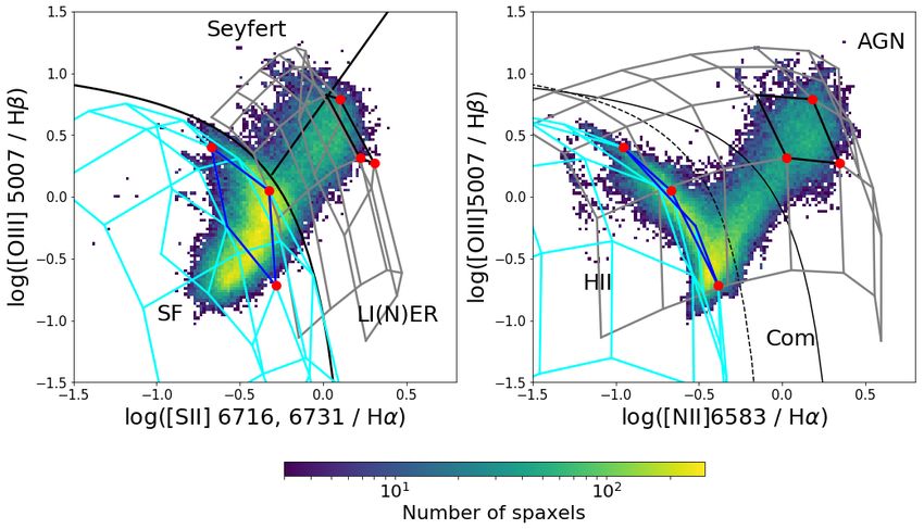
4 X. Ji & R. Yan
line ratios alone and we will group them as LI(N)ERs. We will more ideal to reveal the gap between model surfaces and to separate
discuss these LI(N)ER spaxels and their identification in §5.1. regions with different ionization mechanisms.
 Here we show how to obtain the ideal projection by consecutive
 rotations in the 3D line-ratio space. To begin with, we note that for
 a small enough region on the model grid, the curvature of the
3 NEW PROJECTION FOR THE OPTICAL model surface is negligible. If we have two planes with exactly zero
 DIAGNOSTIC DIAGRAM curvatures, the procedure to find their edge-on projection can be
 summarized as follows:
3.1 Projections from the 3D line-ratio space
 1 Find where the two planes intersect. It will be a straight line in
In Fig. 1, we plot our photoionization models for SF and AGN the 3D space;
together with our sample in an animated three-dimensional line- 2 Find a plane which is perpendicular to this intersection line;
ratio space spanned by N2, S2, and R3. Each photoionization model 3 Find the two axes of this plane. We note that in this step, one
manifests itself as a 2D continuous surface embedded in the 3D has the freedom to change these axes under a rotation about the
space, and each point on the model surface corresponds to a unique intersection line. An easy way to find a set of axes is to perform
set of metallicity and ionization parameter. It is clear that there is two consecutive rotations of the original axes. The direction of the
a gap between the AGN model surface and the SF model surface, intersection line determines a polar angle and an azimuthal angle
indicating that there is no degeneracy between these two ionization . If we start with N2, S2, and R3 as , , and axes, a first rotation
models, at least in the part of parameter space we care about. Line about the axis by an angle and a second rotation about the new
ratios of pure SF or pure AGN have to be located on or near these axis by an angle would directly lead us to the plane (which is
two disjoint model surfaces. Some data points are indeed there. the final 1 − 2 plane).
However, some of the data points lie in the gap, separate from
both model surfaces. They actually form a bridge connecting the Going back to our model surfaces, they are curved surfaces in the 3D
two surfaces. The most natural explanation is that they are indeed diagram. But since we only care about the part of parameter space
‘composite’ objects resulting from a combination of SF and AGN where our sample is located, we can pick out certain patches of the
due to unresolved observations. model surfaces, which will be small enough to be approximated
 In Fig. 2, we show a few 2D projections of this 3D line-ratio by planes. In Fig. 3, we choose one quadrangle patch from each
space. Two of the projections correspond to the traditional [S II]- photoionization model grid. The patch of SF grid covers the part
based and [N II]-based BPT diagrams, while the third one is a new of the parameter space satisfying 0.0 < [O/H] < 0.3 and −2.5 < q
projection we propose. The axes of the new projected 2D diagram < −3.0, and the patch of the AGN grid covers the parameter space
(wihch we denote as 1 and 2 ) are made of linear combinations satisfying 0.0 < [O/H] < 0.25 and −3.0 < q < −3.5. These parts of
of the three line ratios from the two original diagrams, thus having models are chosen as they represent the line ratios of the the most
the same virtue of using only strong lines and being insensitive densely-populated areas by the data in the [N II] and [S II] BPT
to extinction. The advantage of the new diagram compared to the diagrams. The curvature of each patch is relatively small, and we
original ones is that it maximizes the separation between the SF can construct two planes by selecting three points from each of the
model grids and the AGN model grids. In essence, we are choosing quadrangle. Using these two planes, we are able to find the desired
the projection that views both model surfaces roughly edge-on for final plane of projection.
the parts of parameter space that matter. The gap between them Fig. 4 shows how we construct the final plane in the 3D line-
would become even emptier, if one further removes some models ratio space. The polar angle (from the R3 axis) is 36 degree, and
that are not found in the data, judging with the 3rd dimension that is the azimuthal angle (defined as a counter-clockwise angle from
perpendicular to the two dimensions shown here. We will illustrate the positive direction of the N2 axis) is 39 degree.
this below. With the rotation angles determined, we calculate the expres-
 Furthermore, with the model surfaces appearing edge-on, it sions for the axes of this reprojected plane, which are:
becomes easier to directly compare them with the observational 1 = 0.63 N2 + 0.51 S2 + 0.59 R3, (4)
data, in a way that maintains consistency across three line ratios.
It not only enables us to better constrain the input parameters of and
the models, but also provides a way to investigate the contribution 2 = −0.63 N2 + 0.78 S2. (5)
of different ionization sources to the observed line ratios. We will
discuss these applications in §4. In the left panel of Fig. 5, we plot our data and models in this new
 diagnostic diagram. We cut the model grids to keep only those mod-
 els that cover a similar range on the 3 axis (which is perpendicular
 to the 1 − 2 plane in the 3D space) as our data. The information
3.2 Derivation of the axes of the new projection
 from this third dimension further shrinks the spread of the models
Fig. 3 shows the data distribution and our models in the traditional in the 1 − 2 plane. The expression for 3 is:
BPT diagrams. From the 3D perspective, we could view the [N II]
 3 = −0.46 N2 − 0.37 S2 + 0.81 R3. (6)
and [S II] diagrams as two different projections. The AGN model
in the [S II] projection is closer to being ‘edge-on’ while it is nearly We note that one has the freedom to make a translation to the origin
‘face-on’ in the [N II] one. This is why the data distribution in the along the 3 axis, which is equivalent to adding a constant term to
[S II] diagram is more useful for constraining the AGN SED (Ji the above equation. The sample distribution on the 1 − 3 plane is
et al. 2020). By contrast, the [N II] projection works better to isolate shown in the right panel of Fig. 5. 98% of our data lie in the range
pure H II regions, because the SF surface becomes more compact −0.23 < 3 < 0.98. Thus, we keep only the parts of the model
at high metallicity in this diagram. It is natural to imagine that there grids with 3 within this range.
is a projection that make both surfaces edge-on, which would be The final photoionization models appear quite compact in this

 MNRAS 000, 1–16 (2020)

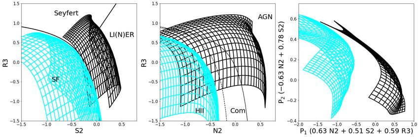
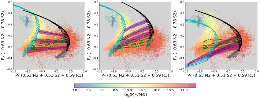
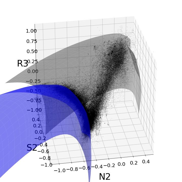
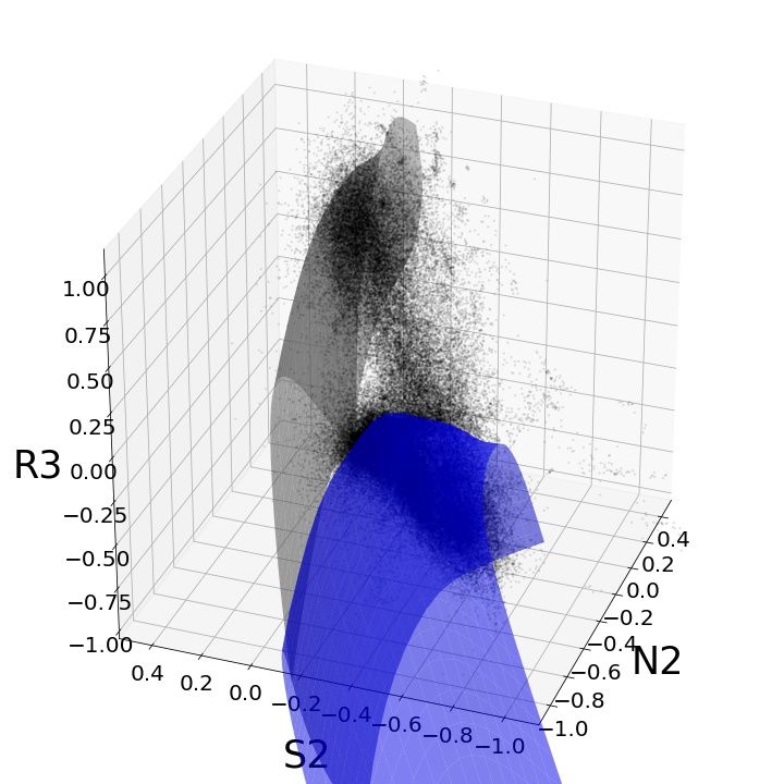
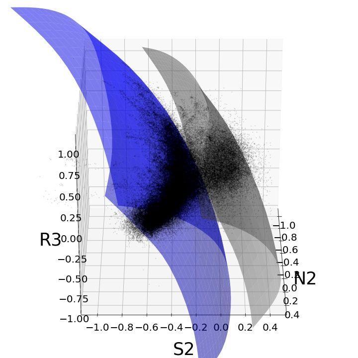
3D Optical Diagnostics 5

Figure 1. Left: a 3D BPT diagram viewed at an elevation angle of 30 degrees. A sample of MaNGA central spaxels with / e < 0.3 are shown as black points.
The SF and AGN models are plotted as the blue and the grey surfaces, respectively. Click on this image in a PDF viewer to make it stop rotating. Middle and
Right: two still images from the animation, illustrating the gap between two model surfaces and how the data points are distributed relative to them.

Figure 2. Comparison of photoionization models in three optical diagnostic diagrams. AGN model grids (black) and SF model grids (cyan) displayed in the
diagrams have been smoothed through interpolation. Left panel: the [S II]-based BPT diagram; middle panel: the [N II]-based BPT diagram; right panel: the
new diagram proposed by this paper.

 1 − 2 projection. This leads to strong constraints on the model coefficients of N2 and S2 for the 2 axis are very close to be
parameters, as the data points for pure AGN-ionized or SF-ionized opposites, making 2 close to the S2N2 ratio, which is a good
clouds should trace the model surfaces. The data show a curved tracer for metallicity (Dopita et al. 2016). Thus, we expect the
locus on the left side, with 1 between −1 and −0.5, which is traced constant metallicity lines in this diagram to have roughly constant
nicely by our fiducial star-forming model. To the right of it, we see 2 values. On the other hand, for the part of the model grids we
a nearly horizontal extension, with a concentration of points around kept, the constant ionization parameter lines have roughly constant
 1 ∼ 0.5. This blob on the right contains the Seyferts and LI(N)ERs 3 values, as is shown in the right panel of Fig. 5. The outcome
identified by the original BPT diagram. Our fiducial AGN model of these facts combined is that each iso-metallicity surface almost
roughly traces the envelope of this blob rather than going through appears as a line parallel to the 1 axis in the regime where our
the densest part of it. This could mean that our fiducial model is not data points are populated, which facilitates the decomposition of
a good description for a typical AGN-photoionized cloud. We will the different ionizing components for our sample, as we will discuss
investigate this in the next section. The stretch of points between in the next section.
the SF locus and the AGN blob are far away from both models. As We list in the following several potential applications of this
we will demonstrate in the next section, they cannot be explained new diagram.
by varying the parameters of the SF model or the AGN model. The
most natural explanation is that they are composites of SF and AGN, 1 Separate the pure SF regions, pure AGN regions, and compos-
due to insufficient spatial resolution of our observations or spatial ite regions with no ambiguity. Since this projection already implic-
projection effects in the target galaxy. itly enforces consistency between the [N II] and [S II] BPT diagrams,
 Another interesting fact of this new projections is that the and significantly reduces the projected areas of theoretical model

MNRAS 000, 1–16 (2020)

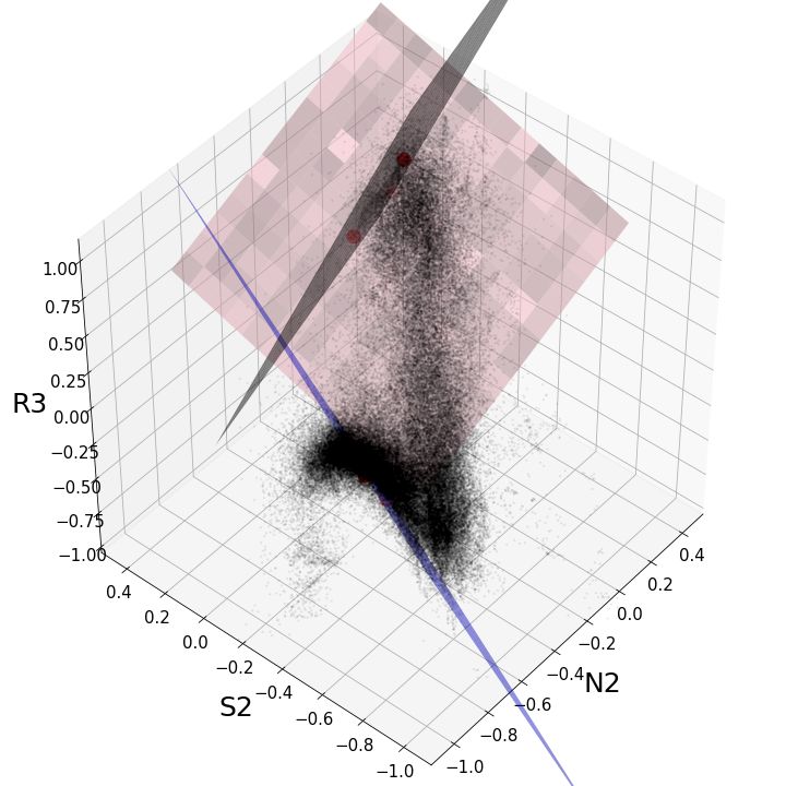
6 X. Ji & R. Yan

Figure 3. Photoionzation models and observational data viewed in the [S II]- and [N II]-based BPT diagrams. The solid black curves are Kewley et al. (2001)
extreme star-burst lines. The dashed black curve in the right panel is the Kauffmann et al. (2003) demarcation that separates H II regions from AGNs. The
solid straight black line in the left panel is the Kewley et al. (2006) line which separate Seyferts from LI(N)ERs. The models used here are described in §2. The
parts of the model grids that are highlighted in black (blue) is the patch we select to represent the AGN (SF) model surface. Red points are chosen to construct
planes in the 3D diagram to find the angle from which both model surfaces are viewed nearly ‘edge-on’.

 grids, data points of pure SF and pure AGN should distribute about
 the projected models, and those of the composite regions should
 lie in the gap between them. One potential uncertainty is that there
 could be variations of the model positions due to different sets of
 model parameters. This point is further investigated in §4.1. The de-
 marcations for different ionized regions in the new diagram based
 on the decomposition of line ratios are given in Section §4.3.
 2 Constrain the photoionization model parameters, like the sec-
 ondary nitrogen abundance and the shape of the ionizing SED. The
 data distribution span a narrow range, less than 0.8 dex, along the
 2 axis, which is very sensitive to the amount of nitrogen included.
 Changing the nitrogen prescription should result in noticeable shift
 of the model relative to the data in the vertical direction, allowing
 one to put strong constraints on the nitrogen prescriptions. On the
 other hand, changing the hardness of the input SED will system-
 atically lower/increase all line ratios. Since the vertical axis tends
 to cancel out the changes in line ratios, the model will move in the
 horizontal direction.
 3 Estimate metallicity for composite regions. For the composite
 regions with line ratios sitting between pure-AGN and pure-SF
 model surfaces, it is potentially possible to construct iso-metallicity
 lines between the two edge-on models and calculate the metallicity
 for each point. However, there is still certain difficulty due to the
 nitrogen prescription inconsistency between the best-fit AGN and
Figure 4. The final plane (pink) constructed from the two model patches SF models. We will illustrate this in §4.2.
(in grey and cyan, respectively). The black (blue) plane is the representative 4 Calculate the contributions of different ionizing sources given
plane for the AGN (SF) model constructed through the red points, and is the corresponding models. Since regions ionized by a single source
perpendicular to the final plane. The black data points are our sample spaxels. should ideally have a very narrow distribution about the correspond-
 ing model surface, we are able to set up a parameterization so that
 every point lying between two different ionizing models can be
 described by the relative contributions from these sources. These

 MNRAS 000, 1–16 (2020)

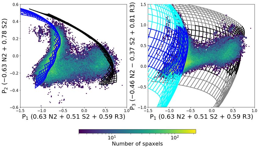
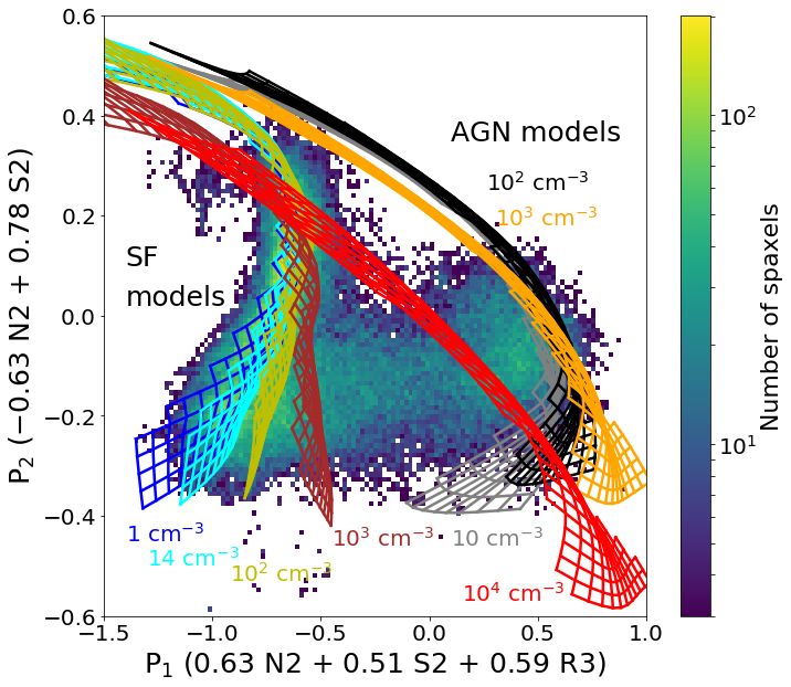
3D Optical Diagnostics 7

Figure 5. Left panel: final plane of projection. The photoionzation models are first interpolated and then cut in the 3 (perpendicular) direction so that they
cover the middle 98% of the data points. Right panel: 1 − 3 plane. Parts of the model grids (in cyan and grey) are cut off according to the distribution of the
data points along the 3 axis. The 2D number density distributions of the our sample spaxels are displayed in both panels.

results can be used to create demarcation lines with a specific thresh- diagram. In particular, we need to find what changes to the AGN
old on the contamination from the other sources. But one should model parameter could lead to a better fit to the densest part of the
be cautious about the assumptions made before decomposing the AGN blob. We will see that the data distribution in this new pro-
sources. jection can place stringent constraints on the models. We consider
 three important inputs to the photoionization models: the hydro-
We will give some preliminary examples of these applications in
 gen density of the cloud, the secondary nitrogen abundance (since
the next section.
 we are using the [N II] emission line), and the shape of the input
 ionizing SED.

4 IMPLICATIONS AND APPLICATIONS OF THE NEW Among the three inputs, the hydrogen density is
 DIAGRAM well constrained by the electron density derived using the
 [S II] 6716/[S II] 6731 ratio of our sample. The PyRAF calcu-
In this section we discuss both the implications and applications of lation gives a median value of 100 cm−3 for the AGN spaxels and
the new projection for the optical BPT diagnostics. 14 cm−3 for the SF spaxels in MaNGA. This is in good agreement
 with the result we obtain by directly comparing the [S II] doublet
 ratios produced by CLOUDY models to the median ratio in the data.
4.1 Constraints on model parameters
 Thus, we do not need to change this assumption. Regardless, we
With our new 1 − 2 projection, we consider that the correct SF illustrate here how density variation will impact the models in our
model should go through the densest part of the SF locus on the left new projection, which demonstrates the power of looking from the
and the correct AGN model should go through the densest part of right angle. Fig. 6 shows this density dependence of the models. At
the AGN blob on the right. There are two reasons. First, the data low metallicities and when density is less than 100 cm−3 for SF or
should show scatters around the model due to intrinsic scatter of 1000 cm−3 for AGN, the models are not sensitive to the densities.
the physical parameters and observational uncertainty on the line But at high metallicities, both the SF and AGN models shift to the
ratios. Second, for the composite objects, the most natural line ratio right with an increasing density. At even higher density, the AGN
distribution of them should pile up at the two end points where one model grid moves downward (at high metallicity) and even to the
component completely dominates over the other. Any concentration lower left (at low metallicity). The movement of the model surface
of data in-between the end points would require an explanation of is mostly due to the temperature dependence of the collisional ex-
why that particular ratio of combination is preferred. Therefore, we citation rates for [S II] and [N II]. The change in direction above
think the densest regions of the SF locus and AGN blob should a density of 1000 cm−3 is due to the collisional de-excitation of
match the pure SF and AGN models, respectively. [S II]. These movements are very significant compared to the data
 Thus, we first examine how the parameters of the photoion- concentration. In the traditional BPT diagrams (see Fig. 11 of Ji
ization model can impact the position of the models in this new et al. 2020 for example), the role of density is much less obvious

MNRAS 000, 1–16 (2020)

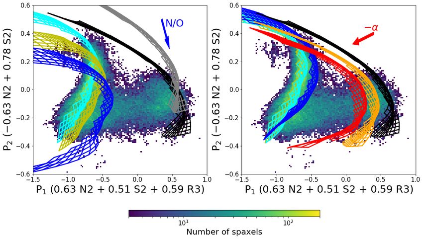
8 X. Ji & R. Yan
because it is all hidden by projection effects due to the non-optimal
viewing angles.
 In comparison to the density, the nitrogen abundance prescrip-
tion is more difficult to measure, which results in significant dis-
agreements in the literature. Though Schaefer et al. (2020) derived
a median N/O ratio vs. metallicity relation for H II regions from
MaNGA, they also find that this relation depends on the total stellar
mass and the local star formation efficiency of the host galaxies. It
is possible that AGN-ionized regions (and/or LIERs) have different
nitrogen enhancement from that of the SF regions, as they are more
likely to be found in more massive and evolved galaxies. In order
to constrain this parameter from the side of theoretical models, we
need to understand how the model grids will move as a whole when
the nitrogen prescription is changed. Qualitatively speaking, as the
nitrogen abundance at a given metallicity increases, the N2 ratio
should increase as well. This makes the model grid move in the
lower right direction, as indicated in the left panel of Fig. 7. The
exact behavior of the model grid might well differ for parts with dif-
ferent metallicities, as can be seen in the case of the AGN models,
where the model also seems to rotate a little bit after we switch its
nitrogen prescription. The two sets of AGN models we plot in this
figure are generated with nitrogen prescriptions adopted by Groves Figure 6. SF and AGN models with various hydrogen densities in our new
et al. (2004a) and Dopita et al. (2013) (we denote them as Dopita13 projected diagram. Our fiducial SF model has a density of 14 cm−3 , and our
prescription and Groves04 prescription hereafter), respectively. The fiducial AGN model has a density of 100 cm−3 . For SF models, we compute
corresponding log(N/O) vs. 12 + log(O/H) relations are shown in four densities from 1 cm−3 to 103 cm−3 , and for AGN models, we compute
Fig. 8, together with some other relations we found in the literature four densities from 10 cm−3 to 104 cm−3 . The densites values are shown by
(cf. Vila Costas & Edmunds 1993; Storchi-Bergmann et al. 1998; the side of the corresponding models. All the models are cut so that they
 enclose the middle 98% of the data along the 3 axis.
Nicholls et al. 2017; Schaefer et al. 2020). We choose these two re-
lations because they yield the highest and the lowest N/O ratios for
all metallicities. The separation between the two sets of model grids
 requires a Groves04 nitrogen prescription and a power-law index of
basically shows the largest difference in line ratios induced by the
 ∼ − 1.7, as shown in the right panel of Fig. 7.
variation in the N/O ratio. For SF regions, we add another model
 If we consider adjusting the nitrogen prescription of the SF
with the nitrogen prescription derived by Schaefer et al. (2020)
 model instead, the SF model with a Groves04 nitrogen prescription
(hereafter Schaefer20 prescription), which gives the second lowest
 would fall too far to the lower right of the SF locus. It seems
N/O ratios for most metallicities as shown in Fig. 8. To fit the SF
 even harder to move it up in the upper left direction by changing
locus traced by the densest part of the data distribution, the lowest
 the density or the shape of the ionizing SED. In the right panel
N/O ratio prescribed by Dopita et al. (2013) is needed. A slightly
 of Fig. 7, we show several SF models with different input SEDs
elevated N/O vs. [O/H] relation like the Schaefer20 prescription
 corresponding to different ages for a starburst with constant star
would be enough to drive the model away from the center of the SF
 formation rate. The models do not differ in their vertical positions at
locus. As a consequence, the SF locus in this diagram puts a strong
 all. According to D’Agostino et al. (2019b), possible variations in the
constraint on the nitrogen prescription for our SF models. On the
 ionizing radiation field of the H II regions from different population
other hand, an AGN model with the Dopita13 prescription would
 synthesis models only introduce an average systematic difference
lie too high to match the AGN blob in our new diagram centered
 of ∼ 0.1 dex in the N2 and R3 line ratios. Thus, varying the input
around 1 ∼ 0.4 and 2 ∼ −0.1.
 SEDs for the SF models also could not resolve this discrepancy.
 As a result, it seems that there is a discrepancy between the best To summarize, solely judging from the distribution of the data
fitting nitrogen prescriptions indicated by the SF and AGN models. in our new diagram, the best-fit SF model has a Dopita13 nitrogen
Raising the hydrogen density of the AGN model to much higher prescription and a continuous SFH no younger than 4 Myr, while
than 1000 cm−3 could lower its vertical position. But this is not a the best-fit AGN model has a Groves04 nitrogen prescription and a
viable solution as it would contradict the measured [S II] doublet power-law index of −1.7. This discrepancy in the nitrogen prescrip-
ratio. tion cannot be easily solved by adjusting other model parameters.
 Another model input we can vary is the SED of the ionizing This discrepancy suggests some assumptions we make in modelling
spectra. The right panel of Fig. 7 shows that by softening the input the ionized cloud must be incorrect, or there are some difference in
SED of the AGN model, we can move the model grid to the left the physical environments around SF and AGN that we have not yet
and slightly downward. An AGN model with a softer SED and the considered in our modeling. We will further discuss this puzzle and
Dopita13 nitrogen prescription could match the upper part of the its consequence in the next section.
AGN blob, but would require unrealistically high metallicity ([O/H]
> 0.75) to cover the bottom part of it. Therefore, varying the SED
would not solve the discrepancy in the nitrogen prescription between 4.2 AGN/SF composites and the iso-metallicity mixing
SF and AGN models. sequence
 In fact, if we use the density distribution of the AGN blob as With the above exploration of how AGN and SF models depend
a metric, to make the AGN model go through the densest part of it on the model parameters and assumptions, we found that none of

 MNRAS 000, 1–16 (2020)

3D Optical Diagnostics 9

Figure 7. Photoionization model grids and the distribution of MaNGA central spaxels in the new diagram. The color-coding of the data indicates the density
of spaxels in the diagram. Left panel: the SF model with the Dopita13 (Groves04) nitrogen prescription is shown in cyan (blue), and the AGN model with the
Dopita13 (Groves04) nitrogen prescription is shown in grey (black). Besides these two extreme prescriptions, the Scheafer20 prescription is used to compute
the yellow model grid for SF regions. The blue arrow roughly indicates how the model grids would move if the overall N/O ratio is increased. Right panel:
AGN models with a Groves04 nitrogen prescription and input SEDs of which the power-law indices are −1.4, −1.7 and −2.0 are shown in black, orange, and
red, respectively. The red arrow roughly indicate in what direction the AGN model grid would move if the power-law index of the input SED is decreased.
SF models generated by SEDs of continuous star-formation history but different ages are plotted as well. The star-forming ages for the blue, cyan, and yellow
models are 0.01 Myr, 4 Myr, and 8 Myr, respectively. All the models are cut so that they enclose the middle 98% of the data along the 3 axis.

those models could completely cover the zone between the SF locus AGN/LIER-ionized clouds and SF-ionized clouds that make up a
and the AGN blob. Thus, the simplest explanation is that these data composite region are spatially close (on scales smaller than the PSF
points are from truly composite regions made up by combining of the observations) and have roughly the same metallicities and
SF-ionized clouds with AGN/LIER-ionized clouds. abundance pattern.
 We would like to clarify what we consider as the correct phys- Given this picture and this assumption, it is now feasible to de-
ical picture for a composite region. We consider that a composite compose the composite regions into AGN and SF components, and
region is composed of spatially close but physically separate clouds at the same time, constrain their metallicities. Our new projection
with different ionizing sources, some are ionized by massive young of the line-ratio space makes these constraints quite apparent and
stars (SF), and others by AGN or whatever source is responsible much less ambiguous than decompositions based on the original
for LIERs or diffuse ionized gas. The spectra of these clouds are [N II]- and [S II]-based diagrams. As long as we can find consistent
combined together due to insufficient spatial resolution of the ob- abundance prescriptions between AGN and SF regions, we can con-
servations or projection effects in the target galaxy, leading to a set nect those AGN models with SF models at the same metallicity and
of line ratios that is intermediate between SF and AGN/LIERs. define iso-metallicity mixing sequences. The fact that the ionization
 We consider that it is unlikely for the spectra of composite parameter is nearly hidden in this 1 − 2 projection means the de-
regions to come from clouds that are ionized by a composite SED composition is nearly independent of the ionization parameters of
made up by comparable fractions of AGN photons and SF photons, the AGN and SF regions.
as it requires fine tuning to make them to be on the same order However, as we discussed in §4.1, we cannot find a single nitro-
of magnitude. Given that radiation flux falls with distance squared, gen prescription to fit both the SF locus and the AGN blob. Without
it is more likely that they differ by orders of magnitude for a ran- such a consistent abundance pattern prescription, we cannot carry
dom location in the galaxy. Thus, a single cloud is nearly always out a self-consistent decomposition and metallicity determination
dominated by one of the ionizing sources. In galaxies with signif- for composites. Regardless, we show here how the iso-metallicity
icant shock ionization, the same principle should apply that each sequences would look like in our new projection, and how they
cloud is dominated by one of the ionization mechanisms rather than compare to the distribution of composite regions, which will fur-
balanced by comparable contributions from more than one. ther demonstrate the tension in the nitrogen prescription between
 Under this physical picture, it is reasonable to assume the the SF and AGN models.

MNRAS 000, 1–16 (2020)

10 X. Ji & R. Yan
 can generate a bundle of such lines describing the overall trend of
 an iso-metallicity mixing sequence.
 Fig. 9 shows three examples of the projected iso-metallicity
 surfaces (or line bundles) with [O/H] = 0.15, 0.30, and 0.45. The
 spread of each line bundle is caused by the variation in the ion-
 ization parameter. To fully utilize the information contained in the
 3D distribution of the data, we re-cut the model grids so that they
 only enclose the middle 98% composite spaxels (i.e. excluding the
 upper part of the SF locus with roughly 3 > 0.4 as shown in the
 right panel of Fig. 5). While the median- and high-metallicity line
 bundles appear nearly horizontal, the low-metallicity line bundle
 show a slightly negative slope. It appears that the composite spax-
 els in MaNGA follow a similar trend as our theoretical iso-[O/H]
 sequences. However, we note that the two ends of the composite
 sequence in the data are not necessarily having the same metallicity
 as they could come from different galaxies.
 A sanity check for whether our models produce a sensible com-
Figure 8. Various nitrogen prescriptions in literature. The Groves04 and the posite sequence is to compare the derived iso-metallicity lines with
Dopita13 are the two prescriptions used in this paper. The solar abundance the overall shape of the composite zone. In Fig. 10, we perform a
is indicated by the black star. The arrow shows the effect of the depletion of more careful comparison by binning our data according to the total
oxygen onto dust grains by 0.22 dex. By default CLOUY assumes that oxygen stellar masses of their host galaxies. This would help identify iso-
depletes by 40% or approximately 0.22 dex, while nitrogen does not deplete. metallicity composite sequences in the data by making sure the two
 ends of them are from similar types of galaxies. The stellar masses
 We begin by setting up a series of parameterized iso-metallicity are drawn from the MaNGA Firefly value-added catalog (Goddard
surfaces (or line bundles) connecting our best fitting AGN model et al. 2017). Within each stellar mass bin, we expect both [O/H]
and SF model in the 3D diagram. Since we adopt different nitrogen and N/O are roughly fixed with small scatters, and the distribution
prescriptions for the AGN and SF models, the ‘iso-metallicity’ here of the spaxels in the composite zone provides the correct slope
really means iso-[O/H], but not iso-(N/O). We show below an exam- for an iso-metallicity line bundle. Here we are assuming that the
ple of how we parameterize a mixing line between a pre-determined mass-metallicity relations for SF galaxies and AGN host galaxies
start point on the AGN surface and an end point on the SF surface. are identical (for a potential counterexample, however, see Thomas
The start point is assumed to have line ratios of a pure AGN region, et al. 2019). The theoretical iso-[O/H] line bundles produced by
which we denote as N2AGN , S2AGN , and R3AGN . Similarly, the our best-fit models all exhibit shallower slopes than those indicated
end point corresponds to a pure SF region with line ratios N2SF , by the median data trends in five different mass bins, which in-
S2SF , and R3SF . Now if we observe the two regions together, the clude most spaxels in the composite zone. To steepen the slopes of
resulting line ratios will change, according to the relative strength these iso-metallicity lines by changing the abundance pattern of the
of the emission lines from different regions. Take N2 as an exam- photoionization models, one could either lower the N/O vs. [O/H]
ple, the observed value N2obs can be calculated using the following relation for the AGN model, or elevate this relation for the SF model.
equation. In the middle and right panels of Fig. 10, we plot the iso-metallicity
 lines using SF and AGN models with consistent nitrogen prescrip-
 ( [N II]/H )AGN + i ([N II]/H )SF tions, Dopita 13 for the middle panel and Groves04 for the right
N2obs = log( ), (7)
 1+i panel. We can see that lowering the N/O ratio raises the position
where is defined as the ratio of the H flux contributed by the SF re- of the AGN model in the diagram, and the resulting slopes of the
gion to that contributed by the AGN region, i.e. ≡ H SF /H AGN . iso-metallicity lines are now steeper compared with the data. A no-
S2obs can be computed using a similar equation. Whereas the equa- ticeable problem with lowering the N/O ratio of the AGN model is
tion of R3obs involves the SF-to-AGN ratio for H flux, which we that the composite zone cannot be fully covered. Since the SF locus
denote as . Note is not necessarily the same as because the only reaches a highest [O/H] of 0.5 according to our SF model, if
SF-ionized clouds and the AGN-ionized clouds could have very we only consider the corresponding part of the AGN model (which
different dust extinction, although they are spatially close. To relate is colored in black), even the iso-metallicity line bundle with the
 and , we need to assume a ratio between the Balmer decrement for highest [O/H] could not overlap with the lower part of the mixing
the AGN clouds ( AGN ) and that for the SF clouds ( SF ), which we branch. On the other hand, if we raise the N/O ratio of the SF model
denote as Θ ≡ AGN / SF = / . We can make a simplification by instead, as is shown in the right panel of Fig. 10, the slopes indicated
choosing a constant value for Θ. By taking the ratio of the median by our models for the composite zone are again too steep, and the
Balmer decrement among the AGN regions to that among the H II SF model does not match the SF locus in the data.
regions in our sample, we obtain a representative value of 1.35 for To summarize, the nitrogen prescription for the SF model is
Θ. We will use this value in the following analysis, i.e. = 1.35 . strongly constrained by this SF locus, as we have already seen in
Difference in Θ would lead to a different decomposition result but §4.1. However, in order to cover the AGN blob in the data, the AGN
will not shift the iso-metallicity sequence significantly. model needs a prescription with higher N/O ratios, which results in
 As a result, there is effectively one parameter for constructing an inconsistency in the abundance pattern to explain the composite
a single mixing sequence that connects a start model point and an galaxies. Furthermore, forcing the SF and AGN models to have the
end model point. We can parametrize this sequence by changing same N/O prescriptions makes the iso-metallicity mixing-sequences
log( ) from −∞ to ∞. By varying the ionization parameter of the to be too steep compared to the trends of composite galaxies with
start model point and the end model point at fixed metallicity, we fixed stellar masses. It could be due to incorrect assumptions or

 MNRAS 000, 1–16 (2020)

3D Optical Diagnostics 11
 negligible influence on the decomposition result. Since we currently
 cannot settle the nitrogen discrepancy while matching the models
 to the data, there should be no self-consistent way to decompose the
 data either. Still we would like to show in the following a demon-
 stration of the decomposition using our best-fit SF and AGN models
 (the set shown in the left panel of Fig. 10). Given that these models
 can well describe the majority of the AGN and SF spaxels, they
 should not be far from the correct models. But the correct mod-
 els could have different slopes for the iso-metallicity lines. Judging
 from the left panel of Fig. 10, the bias on AGN due to different
 slopes of the iso-metallicity lines should not be too significant.
 In Fig. 11, we plot the derived AGN as a function of the position
 along the 1 axis. Due to the spread induced by the variation in the
 metallicity and the ionization parameter, the relation has relatively
 large uncertainties at both small 1 values and large 1 values. Part
 of the data points also seem to cluster at discrete values of AGN ,
 which might be due to our insufficient sampling of log . Despite
 the spread, we can see that AGN increases more rapidly as 1 gets
 larger, but quickly plateaus after 1 reaches 0.3, which is roughly
 the horizontal position of the lower part of the AGN model. The
 correlation between AGN and 2 , or that between AGN and 3 , is
 much weaker.
Figure 9. Examples of iso-metallicity line bundles constructed from the
 If the Balmer decrement ratio Θ is changed, the horizontal
photoionization models. The dashed lines are the median trends of line
bundles with different metallicities. The colored shaded regions represent
 position of each parametrized point would change accordingly. In-
the projected areas within one stander deviation from the median along the creasing Θ would shift the model points to smaller 1 values, hence
vertical axis. increasing the overall fitted AGN of our sample. For example, if the
 Θ in our setting is doubled (i.e. Θ = 2.70 in this case), the fractional
 change in the derived AGN of our sample has a median value of
missing physics in our photoionization models, and we will inves- 12%, and the the values for the 16 percentile and the 84 percentile
tigate this issue with more sophisticated photoionization models in of the data are 2% and 22%, respectively. One may wonder if we can
future work. Regardless, this illustrates nicely the power of our new use the observed Balmer decrement to put constraints on Θ. This is
projection of the line ratio space. not sufficient because the observed Balmer decrement also depends
 on the Balmer decrement in the SF-ionized clouds, SF . Therefore,
 adding this additional constraint does not remove the need to make
4.3 Decomposition of the ionized regions one assumption. In principle, if two additional dust-sensitive line
In the previous section we introduce a way to construct iso- ratios were added as extra constraints, it would be possible to solve
metallicity line bundles (or surfaces) between the AGN and SF for both SF and Θ.
model grids, assuming the Balmer decrement ratio, Θ, is fixed. As Fig. 12 shows a map of all MaNGA central spaxels color-
a result, there is effectively one free parameter that determines the coded by the average AGN of each line-ratio bin. With this map,
position of a point on a given iso-metallicity line, which we can we can generate demarcation lines that correspond to a constant
choose to be the ratio of the H flux from the SF-ionized clouds to fractional contribution to the total H flux by AGN-ionized clouds.
that from the AGN-ionized clouds, . Alternatively, we can use to The dashed blue line corresponds to AGN ∼ 0.10, which means
derive another physical parametrization. The fractional contribution the spaxels to their left have a maximum contamination of 10%
to the total H flux by the AGN-ionized clouds is H AGN / H total from AGN-ionized clouds. Similarly, the spaxels to the right of the
= 1/(1 + ), which we denote as AGN hereafter. This parameter tells dotted-dashed black line have a maximum contamination of 10%
us how significant the contribution from AGN-ionized clouds is in from SF-ionized clouds. We can fit 1 as a quadratic function of 2
a composite spectrum. for these demarcation lines. The functional form of the demarcation
 The decomposition process is summarized as the following. line that identifies SF-dominated regions is
First, using a pair of pre-determined SF and AGN models, we con- 1 < −1.57 22 + 0.53 2 − 0.48 (for − 0.4 . 2 . 0.1), (8)
struct all possible iso-metallicity lines (for all ionization parame-
ter combinations), with the parameter ranging from 10−3 to 103 and the functional form of the demarcation line that identifies AGN-
equally spaced in the logarithmic space. For each data point, we dominated regions can be written as
compute the probability distribution of the models using Bayesian
 1 > −4.74 22 − 1.10 2 + 0.27 (for − 0.4 . 2 . 0.1). (9)
statistics, assuming a flat prior (i.e. equal prior probability for all
model grid points). We compute the likelihood of each data spaxel These demarcations are largely determined by the spaxels inside
given each model point in the original 3D parameter space (N2, S2, the composite zone, and therefore should only be applied when
R3) with the uncertainty in these three line ratios (in log). We do −0.4 . 2 . 0.1. From the map (and also Fig.11), we can see that
the calculation in the original 3D space as there is less covariance the AGN fraction AGN drops more rapidly near the start points of
among them than there is among 1 , 2 , and 3 . Given the result- the AGN model. The demarcation lines for AGN regions are largely
ing probability distribution of the models, we compute the expected determined by the location of the best-fit AGN model grid. In the
value for log and convert it to AGN for each spaxel. right panel of Fig. 12, we compare these two demarcations with
 The choice of photoionization models will have a non- the density distribution of our sample. While SF demarcation line

MNRAS 000, 1–16 (2020)