The Limits of Simplicity: Toward Geocomputational Honesty in Urban Modeling

The Limits of Simplicity: Toward Geocomputational
                     Honesty in Urban Modeling
                                    Keith C. Clarke
                            Department of Geography/NCGIA
                           University of California, Santa Barbara
                                 Santa Barbara, CA, USA.
                                Telephone: 1-805-893-7961
                                   FAX: 1-805-893-3146
                              Email: kclarke@geog.ucsb.edu

     Abstract
     Occam's razor informs us that simpler models are better. Yet models of
     geographical systems must often be complex to capture the richness of the human
     and natural environments. When critical decisions, such as those affecting human
     safety, depend on models, the model must be sufficient for the task, yet can
     become impossible for all but the modeler to understand holistically. This paper
     outlines five model components, and examines how a move toward simplicity
     impacts each, focussing on the critical stage of model calibration. Three model
     applications to the same data are examined in terms of how their calibrations took
     place. A comparison of the results shows that model outcomes are subjective, and
     more shaped by their role in decision-making than by scientific criteria. Model
     reduction, a goal as yet lacking methods, may therefore not be a useful way
     forward for geocomputational modeling until the full context of models and the
     ethics of modeling are better understood.

1. Introduction
A model is an abstraction of an object, system or process that permits knowledge to be
gained about reality by conducting experiments on the model. Constraining modeling to that
of interest to the geographer, a model should abstract geographic space and the dynamic
processes that take place within it, and be able to simulate spatial processes usefully. At the
absurd extreme, a model could be more complicated than the data chosen to represent the
spatio-temporal dynamics in question. Occam's razor tells us, of course, that when two
models are of equal explanatory power, the simpler one is preferred. Einstein stated that "a
model should be as simple as possible and yet no simpler." Some earth systems are so
predictable that they are indeed amenable to modeling with the simplest of models. For
example, the drop in atmospheric pressure as a function of elevation is so predictable as to be
suitable for building a measuring instrument for the latter using the former as a proxy. Of
course few human systems, or coupled human/environmental systems are this simple.
Geography's past is laced with attempts to use overly simple predictive or explanatory
models for human phenomena, the gravity model being a good example. In some cases, the
simplicity these models offer serves to produce insight, or at least fill textbooks, in the
absence of geographic laws. In this paper, I raise the issue of model simplicity, and discuss
Einstein's question of how much simplicity is enough.

2. Simplicity in Models
The problem of model simplicity is that models have multiple components and are often
complicated. Complex systems theory has shown that even simple models can produce
complexity and chaos when given the right initial conditions or rules, though gives little
guidance on how to invert this sequence. Formally, models are sets of inputs, outputs, and
algorithms that duplicate processes or forms. The more complicated the process or form, the
less simple a model can be.
Models have been thought of as consisting of four components. These are (1) input, both of
data and parameters, often forming initial conditions; (2) algorithms, usually formulas,
heuristics, or programs that operate on the data, apply rules, enforce limits and conditions,
etc.; (3) assumptions, representing constraints placed on the data and algorithms or
simplifications of the conditions under which the algorithms operate; and (4) outputs, both of
data (the results or forecasts) and of model performance such as goodness of fit. Considering
modeling itself requires the addition of a fifth component, that of the modeler, and including
their knowledge, specific purpose, level of use, sophistication, and ethics. By level of use, we
distinguish between the user who seeks only results (but wants credible models and
modelers), the user who themselves run the model, the user who seeks to change the model,
and the user who seeks to design a model. We term the former two secondary users, since the
model is taken as given. The latter two are primary users, and include modelers.
Communication between primary and secondary users usually consists of model
documentation and published or unpublished papers, manuals, or websites.
Spatial inputs and outputs are usually maps, and the algorithms in Geography and
Geographic Information Science usually simulate a human or physical phenomenon, changes
in the phenomenon, and changes in its cartographic representation. Modeling itself, however,
is a process. A modeler builds data or samples that describe the inputs, selects or writes
algorithms that simulate the form or process, applies the model, and interprets the output.
Among those outputs are descriptions of model performance, forecasts of unknown outputs,
and data sets that may be inputs to further models.
Why might it be necessary to seek the limits of simplicity? I illustrate why using a practical
example of immense environmental significance in the United States, that of the Yucca
Mountain high level radioactive waste disposal site in Nevada. The problem requiring
modeling is that of finding a permanent, safe and environmentally suitable storage location
for the thousands of tons of highly radioactive waste from decades of civilian and military
work in nuclear energy. The specifications of this site are that it should remain “safe” for at
least 10,000 years. Safety is defined by the level of radionuclides at stream gaging stations a
few kilometers downstream from the location. Failure in this case could be at least nationally
catastrophic, and safety depends on the waste remaining dry. The recommendation to bury
the waste deep underground dates back to 1957. The selection of the Yucca Mountain site
came after a very lengthy process of elimination, debate over safe storage and studies by the
regulatory agencies and the National Academy of Science. Scientists at the Los Alamos
National Laboratory in the Earth and Environmental Sciences division took on the task of
using computer simulation to approach the problem of long term stability at the site.
Simple risk assessment methodology uses probability distributions on the random variables
and perhaps Monte Carlo methods to gain knowledge of the overall probability of failure. As
the models become more complex, so also does the probability density function. In 1993 a
study reporting the detection of radionuclides from Cold War era surface nuclear testing in

the deep subsurface at Yucca Mountain introduced the immense complexity of modeling sub-
surface faults and so-called “fast hydrographic pathways” (Fabryka-Martin et al., 1993).
With the earliest, more simple, models the travel times of radionuclides to the measurement
point was about 350,000 years. Adding Dual Permeability, allowing rock fracture, generated
a new and far more complex model that showed travel times to only tens to hundreds of
years, thereby failing the acceptance criterion. Although more complex, these models are
more credible because they can duplicate the data on the fast hydrographic pathways.
Nevertheless, highly complex models become cumbersome when dealing with the public
decision making process. Robinson (2003) notes that for a numerical model to be useful in
decision making, it must be correct and appropriate to the questions beings asked from the
point of view of the scientists and model developers, and understandable and believable from
the perspective of decision makers. A report noted that “...the linkage between many of the
components and parameters is so complex that often the only way to judge the effect on
calculated results of changing a parameter or a submodel is through computational sensitivity
tests.” (NWTRB, 2002). The latest model, called TSPA-LA, has nine major subcomponent
models with nine interacting processes, and a total of 70 separate models, each with multiple
input and complex interconnectivity. Some components are apparently similar (e.g. Climate
inputs and assumptions), but interact in complex ways (in this case through unsaturated zone
flow and saturated zonal flow and transport). Some submodels produce outputs that enter into
macro-level models directly, while in other cases the same values are inputs for more models,
such as those related to disruptive events.
In such a case, does any one person comprehend the entire model, even at a superficial level?
How can it be proven that one or more variables actually contributes to the explanatory
power of the model? More important, how can scientists establish sufficient credibility in
such a complex model that sensible (or even any) political decisions are possible, especially
in a highly charged decision-making environment? Los Alamos scientists have undertaken a
process of model reduction as a consequence. Model reduction is the simplification of
complex models through judicious reduction of the number of variables being simulated.
Methods for model reduction do not yet exist, and deserve research attention. For example,
when does a complex model pass the layman understandability threshold, and when it does,
how much of the original model's behavior is still represented in the system? What variables
can be made constant, and which eliminate or assumed away altogether? How much
uncertainty is introduced into a model system by model reduction? In statistics, reducing the
sample size usually increases the uncertainty. Is the same true at the model level? What are
the particularly irreducible elements, perhaps the primitives, of models in which geographic
space is an inherent component? Such questions are non-trivial, but beg attention if we are to
work toward models that hold the credibility of their primary and secondary users.

3. Honesty in Models and Modeling
Sensitivity testing is obligatory to establish credibility in complex models. Sensitivity tests
are usually the last stage of model calibration. The modeler is also usually responsible for
calibrating the model, by tinkering with control parameters and model behavior, and at least
attempting to validate the model. While validation may actually be impossible in some cases
(Oreskes et al, 1994), calibration is obviously among the most essential obligations of
modeling. Model calibration is the process by which the controlling parameters of a model
are adjusted to optimize the model's performance, that is the degree to which the model's
output resembles the reality that the model is designed to simulate. This involves necessarily
quantitative assessments of the degree of fit between the modeled world and the real world,

and a measurement of the model's resilience, that is how sensitive it is to its input, outputs,
algorithms, and calibration. That the obligation to make these assessments is that of the
modeler is part of what the authors of the Banff Statement termed "Honesty in modeling"
(Clarke et al., 2002).
Such an approach could be considered an essential component of modeling ethics generally,
and even more so in Geography where the real world is our target. Uncalibrated models
should have the status of untested hypotheses. Such is not often the case, however. Even
reputable peer reviewed journals occasionally publish papers on models that are only
conceptual, are untested, or tested only on synthetic or toy data sets. These papers are often
characterized by statements such as “a visual comparison of the model results”, or “the
model behavior appears realistic in nature.” Assumptions go unlisted, limitations are
dismissed, data are used without an explanation of the lineage or dimensions, and fudge
factors sometimes outnumber model variables and parameters. A common practice is to use
values for parameters that are “common in the literature”, or looked up from an obscure
source. The earth's coefficient of refraction for the atmosphere, or example, has long been
assumed to be 0.13, a value derived from the history of surveying. This number is a gross
average for a value known to vary form 0.0 to 1.0 and even beyond these limits under
unusual circumstances such as in a mirage.
While simplicity in model form is desirable, indeed mandatory, what about simplicity in the
other four components of modeling? Simplicity is inherent in the model assumptions, as
these are often designed to constrain and make abstract the model's algorithms and formulas.
Simplicity is not desirable in inputs, other than in parameter specification, since the best
available data should always be that used, although usually data are often determined by the
processing capabilities. Data output is often also complex, and requires interpretation,
although our own work has shown that simple visualizations of model output can be highly
effective, for example as animations. Part of data output are performance data. Should there
be simplicity in calibration and sensitivity testing? Reviews of the literature in urban growth
modeling (e.g. Agarwal et al., 2000; Wegener, 1994; EPA, 2000), show that precious few
models are even calibrated at all, let alone validated or sensitivity tested. Most common is to
present the results of a model and invite the viewer to note how "similar" it is to the real
world. Such a lack of attention to calibration has not, apparently, prevented the models
widespread use. Doubts are often assumed away because the data limitations or tractability
issues exceed these as modeling concerns.
If one uses the argument that we model not to predict the future, but to change it, then such
concerns are perhaps insignificant. The development of new models obviously requires some
degree of trial and error in model design. Models are also testbeds, experimental
environments, or laboratories, where conceptual or philosophical issues can be explored (e.g.
McMillan, 1996). This is often the case with games, in which some models are intended for
education or creative exploration. Such uses are similar to the link between cartography and
visualization; or science and belief. These uses are not, strictly, of concern in science.
Science based models have to work in and of themselves. Methods for model calibration
include bootstrapping and hind casting. If models are to be used for decisions, to determine
human safety in design, or to validate costly programs at public expense, then clearly we
need to hold models to a more rigorous, or at least more valid, standard. Such issues are of no
small importance in geographical models, and in geocomputation at large. Even minor issues,
such as random number generation (Van Niel and Leffan, 2003), can have profound
consequences for modeling. Whether or not model algorithms and code are transparent is at
the very core of science: without repeatability there can be no verification at all.

4. A Case Study
The simplicity question, therefore, can be partially restated in the context of this paper as:
what is the minimum scientifically acceptable level of urban model calibration? Whether this
question can be answered in general for all models is debatable. A complete ethics code for
modeling is obviously too broad for a single paper. We therefore stick to urban models and
issues of calibration and sensitivity testing. This paper examines the problem for a set of
three models as applied to Santa Barbara, California. The three models are the SLEUTH
model (Clarke et al., 1997; Clarke and Gaydos, 1998), the WhatIf? Planning model by
Richard Klosterman (1997), and the SCOPE model (Onsted, 2002). Using the case study
approach, the three models are analyzed in terms of their components, their assumptions, and
their calibration processes. As a means of further exploring the consequences of modeling
variants, their forecasts are also compared and the spatial dissimilarities explored in the light
of the data for Santa Barbara.

4.1 The SLEUTH Model
SLEUTH is a cellular automaton (CA) model that simulates land use change as a
consequence of urban growth. The CA is characterized by working on a grid space of pixels,
with a neighborhood of eight cells of two cell states (urban/non urban), and five transition
rules that act in sequential time steps. The states are acted upon by behavior rules, and these
rules can self modify to adapt to a place and simulate change according to what have been
historically the most important characteristics.
SLEUTH requires five GIS-based inputs: urbanization, land use, transportation, areas
excluded from urbanization, slopes, and hillshading for visualization. The input layers must
have the same number of rows and columns, and be correctly geo-referenced. For statistical
calibration of the model, urban extent must be available for at least four time periods.
Urbanization results from a "seed" urban file with the oldest urban year, and at least two road
maps that interact with a slope layer to allow the generation of new nuclei for outward
growth. Besides the topographic slope, a constraint map represents water bodies, natural and
agricultural reserves. After reading the input layers, initializing random numbers and
controlling parameters, a predefined number of interactions take place that correspond to the
passage of time. A model outer loop executes each growth history and retains statistical data,
while an inner loop executes the growth rules for a single year.
The change rules that will determine the state of each individual cell are taken according to
the neighborhood of each cell, those rules are: 1. Diffusion, 2. Breed, 3. Spread, 4. Slope
Resistance, and 5. Road Gravity. A set of self-modification rules also control the parameters,
allowing the model to modify its own behavior over time, controlled by constants and the
measured rate of growth. This allows the model to parallel known historical conditions by
calibration, and also to aid in understanding the importance and intensity of the different
scores in a probabilistic way. The land use model embedded within SLEUTH is a second
phase after the growth model has iterated for a single pass, and uses the amount of urban
growth as its driver. This model, termed the deltatron (Candau and Clarke, 2000), is tightly
coupled with the urbanization model. The dynamics of the land cover change are defined
through a four-step process in which pixels are selected at random as candidate locations and
changed by a series of locally determined rules largely controlled by proximity and the land
cover class transition matrix. Forecasts can be for either urban growth alone (Figure 1), or for

land cover forecasts and their associated uncertainty (Candau, 2000a).
SLEUTH is public domain C-language source code, available for download online. It is not
suitable for systems other than UNIX or its variants. A sample data set (demo_city) is
provided with a complete set of calibration results. A full set of web-based documentation is
on line at http://www.ncgia.ucsb.edu/projects/gig.

 Figure 1: Forecast urban growth for Santa Barbara in 2030 using SLEUTH. Yellow was urban in 2000.
  Red is urban with 100% probability in 2030. Shades of green are increasing urban, starting at 50%.

4.2 SLEUTH Calibration
SLEUTH calibration is described in detail in Clarke et al. (1996) and Silva and Clarke
(2002). This “brute force” process has been automated, so that the model code tries many of
the combinations and permutations of the control parameters and performs multiple runs
from the seed year to the present (last) data set, each time measuring the goodness of fit
between the modeled and the real distributions. Results are sorted, and parameters of the
highest scoring model runs are used to begin the next, more refined sequences of
permutations over the parameter space. Initial exploration of the parameter space uses a
condensed, resampled and smaller version of the data sets, and as the calibration closes in on
the "best" run, the data are increased in spatial resolution. Between phases in the calibration,
the user tries to extract the values that best match the five factors that control the behavior of
the system. Coefficient combinations result in combinations of thirteen metrics: each either
the coefficient of determination of fit between actual and predicted values for the pattern
(such as number of pixels, number of edges, number of clusters), for spatial metrics such as
shape measures, or for specific targets, such as the correspondence of land use and closeness
to the final pixel count (Clarke and Gaydos, 1998). The highest scoring numeric results from
each factor that controls the behavior of the system from each phase of calibration feed the
subsequent phase, with user-determined weights assigned to the different metrics. Calibration
relies on maximizing spatial and other statistics between the model behavior and the known
data at specific calibration data years. Monte Carlo simulation is used, and averages are
computed across multiple runs to ensure robustness of the solutions.
Recent work on calibration has included testing of the process (Silva and Clarke, 2002), and
testing of the temporal sensitivity of the data inputs (Candau, 2000b). Candau's work showed
that short term forecasts are most accurate when calibrated with short term data. Silva and
Clarke showed that the selection process for the "best" model results is itself an interpretation
of the forces shaping urbanization in a region. Recent work on Atlanta (Yang and Lo, 2003)
has shown that the calibration process steps that take advantage of assumptions of scale
independence are invalid, meaning that ideally the calibration should take place exclusively
at the full resolution of the data. Discussion of these findings has sometimes taken place on
the model's on-line discussion forum.

4.3 The SCOPE model
The South Coast Outlook and Participation Experience (SCOPE) model was originally based
on the UGROW model, adapted and rebuilt in PowerSim and eventually rebuilt again at
UCSB by graduate student Jeffrey Onsted in the STELLA modeling language (HPS, 1995;
Onsted, 2002). SCOPE is a systems dynamics model in the Forrester tradition (Forrester,
1969). This type of model posits simple numerical relations between variables that can be
simulated with basic equations that link values. STELLA allows these empirical relations to
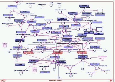
be represented in a complex but logically consistent graphic system, that uses icons and a
basic flow diagram to build the model (Figure 2). Variables can be stocks and flows, with
measurable interactions with finite units, or factors influencing rates and flows but not
contributing to them directly.

                      Figure 2: Sample STELLA code from the SCOPE model

The SCOPE model consists of hundreds of variable-to-variable links, expressed by
equations. Each of these involves its own set of assumptions. These assumptions can be
documented in the model code itself, and in SCOPE's case are also contained in the model's
documentation. The complete set of individual assumptions is immense, and many
assumptions are simply minor variants on relations and rates separated for one of the five
economic sectors in the model (population, quality of life, housing, businesses and jobs, and
land use). The housing sector is further divided into low, middle and upper income, students
and senior citizens. In essence, a separate model is maintained for each, with some
assumptions enforced to keep aggregates the sum of their parts. The model, when complete,
can be used at several levels. At the modeler level, actual parameters and links can be
modified and the program used to generate statistical output in the form of charts and tables.
At the user level, the model has a STELLA interface that allows users to turn on and off
aggregate impacts, such as the application of particular policies, enforcement of rules and
zoning, and sets of assumptions leading to the particular scenarios being developed by the
model's funders. This is done using graphical icons representing switches. At a third and
higher level, this interaction can take place across the world wide web
(http://zenith.geog.ucsb.edu). A last level uses only the scenarios developed through both this
and the SLEUTH model to interact with integrated planning scenarios
(http://zenith.geog.ucsb.edu/scenarios). The SCOPE model is proprietary in that it was
funded as a local not-for-profit project by the Santa Barbara Economic Community Project.

Nevertheless, the model is on-line, and so can be examined in totality, as can the assumptions
behind the model and formulas used. STELLA is a proprietary modeling environment, but is
common in educational environments, and is subsidized for students.

4.4 SCOPE Calibration
SCOPE's original and secondary design were public participatory experiments. A series of
meetings were conducted with various local stakeholder and citizens groups, including
planners, local activists, the general public, and many others while the model was partially
complete to solicit input on what variables were important and how they were best modeled.
This was a long and arduous process, involving hundreds of hours of work, but the result was
encouraging in that when users understood the model and its assumptions, they had high
credibility in its forecasts, even when they were counterintuitive. For example, SCOPE's
demographic module consistently projected population decline in the region over the next
few years, a fact at first rejected and later accepted by the users.
Obviously no user and few modelers can understand the whole SCOPE model. Nevertheless,
the highly graphic STELLA modeling language and its different user interfaces meant that all
users could zoom into and get specific about critical parts of the model from their
perspective. Separate workshops were eventually held to work separately on the major
sectors of the model. Final integration was largely a guided trial and error undertaking, with
the constraint that as one component changed a single calibration metric was used, that of the
Symmetrical Mean Absolute Percent Error (SMAPE) (Tayman and Swanson 1999). Onsted
(2002) stated “We considered an output “validated”, at least for now, if it had a SMAPE of
less than 10%.” This type of calibration has been called "statistical conclusion validity", a
type of internal validity, described by Cook and Campbell as "inferences about whether it is
reasonable to presume covariation given a specified level and the obtained variances" (Cook
and Campbell, 1979, p. 41). While such an approach is similar to bootstrapping, in SCOPE's
case rather extensive sets of historical data on a large number of the attributes being
simulated were available and could be used for SMAPE calculations. Continued refinements
have since improved on the original calibration results. Onsted (2002) conducted a sensitivity
test of sorts, providing a comprehensive bias and error table, and considering the impacts of
the errors on forecasts.

4.5 WhatIf?
The WhatIf? Modeling system was developed by Richard Klosterman and colleagues at the
University of Akron. He describes the system as “an interactive GIS-based planning support
system that supports all aspects of the planning process: conducting a land suitability
analysis, projecting future land use demands, and evaluating the likely impacts of alternative
policy choices and assumptions.” (Klosterman, 1997). The suite of software that constitutes
the model is built on top of ESRI's ArcGIS using MapObjects and Visual basic. The software
is proprietary, and available from Klosterman's consultancy via their web site
(http://www.what-if-pss.com).
For this experiment, a software license was obtained and the data for Santa Barbara,
equivalent to the above project, compiled into the ArcView shape files necessary for WhatIf?
Data preparation in WhatIf? consists of bringing into the software a large number of data
files that contribute to the weighted selection by overlay of the vector polygons that meet
various criteria. Initial preparation consists of selecting the layers, creating their union, and
eliminating errors such as sliver polygons. This creates a set of Uniform Analysis Zones
(UAZs) that are used as the granularity of analysis. Land suitability for urban use (high and

low density residential, and commercial/industrial) are then computed using standard
weighted overlay multicriterion decision making methods. The land suitability method was
Rating and Weighting (RAW), using current land use, distances to roads, streams, the
coastline and commercial centers, topographic slope, the 100 year floodplain, and preserving
agricultural landue. The user must select the weights, based on prior experience or intuition,
and the result is a land suitability map (Figure 3). These maps find their way into an
allocation routine that determines future demand for each use (based on exogenous
estimates), and assigns development based on probabilities calculated from the weights. The
result is a land suitability map, and maps showing development under different assumptions
and scenarios about allocations. The software comes on a CD, which also contains data for a
simulated data set (Edge City).
The approach was applied to Santa Barbara and used for the land suitability stage only. The
software distinguishes between drivers (the growth projection and demand) and factors (the
land suitability and assessment, and the land supply). A third stage, allocation, brings
demand and supply together. Thus our application used only part of the software, which is a
full planning support system. Results are shown in figure 3. Considerable effort was placed
into getting the same data as used in SCOPE and SLEUTH into the WhatIf? simulation.

                 Figure 3: WhatIf? land suitability assessments for Santa Barbara

4.6 WhatIf? Calibration
The WhatIf? documentation contains no information at all about calibration. References are
made to models that use the multicriterion weighted overlay method, such as CUF II (Landis
and Zhang, 1998) and MEPLAN (Echenique et al., 1990). This tradition goes back to the
work of McHarg and Lowry within planning, and is an established approach. The modeling,
or rather forecasting, is an allocation of an exogenous demand using spatially determined
input criteria such as buffers, thematic layers, exclusion areas, and other factors.
To be fair, the planning approach of What If? is based on assuming an invariant present and
an almost absent past. In the application, past twenty-year decadal population totals were
used to make linear projections of future population as part of the housing demand
estimation, but these were totals only and not spatially disaggregated. Thus the intelligence
passes from the explicit assumptions of the model to the skills and experience of the modeler
in compiling accurate input data, in selecting and computing weights, and in combining the
requisite layers effectively. Forecasting routines are more deterministic, and even the number
of forecast periods is prescribed. Thus every time the model is applied to a new area, its
application is completely customized, and while reproducible, is rarely sufficiently
documented that the same results would be attained even from the same data. Thus the model
relies entirely on the credibility of the input data and the acceptability of the results. The
actual code is compiled, and while the principles are demonstrated clearly in the
documentation, the actual executable code is black-box.

5. Model Comparisons

Each of the models applied to Santa Barbara produced a forecast for the year 2030.
Comparison between the models can only take the form of a matching of forecasts, since the
actual future distribution and amount of housing in Santa Barbara in 2030 remains unknown.
Thus we can “simply” compare the models to each other. One of the few values that is an
estimate in common among the forecasts is the additional area of built up land. These directly
comparable values are listed in table 1.

   Table 1: Comparison of model results for additional developed area in Santa Barbara (2000-2030)
                                 WhatIf?                         SCOPE                         SLEUTH
New urban area (ha)                           14006                            4856                            2047
Assumptions             All commercial and residentialBase-line scenario assumed (allBase line as SCOPE. All pixels
                        needs are filled              existing plans followed)       with chance of urbanization > 50%
                                                                                     assumed to become urban
It should be pointed out that even these forecasts have so many caveats as to be mostly
incomparable. The WhatIf? forecasts come from the “What if? growth report, generated by
the software during forecasting. The value is a sum for separate numbers for low density,
high density, medium density and multi-unit housing, plus commercial and industrial land.
Of this area, far more is allocated to commercial/industrial than to residential by 8343.5 to
5662.8 hectares. It was unclear how applying an exogenous demand estimate would change
these values. Spatially, commercial growth was allocated near existing areas of that land use
and particularly in Carpinteria (furthest east) and Goleta (west). High density residential
followed the same pattern, while low density residential was more scattered.

The SCOPE forecasts were generated by flipping the “base-line” policy switch, thus in a
black-box fashion incorporating all of the general plan assumptions that go along with this

prebuilt scenario. These are listed as follows: “The Baseline scenario assumes that the
current urban limit line and other boundaries shall remain unchanged. Also, the South Coast
will continue to build out as outlined in existing General Plans, Local Community Plans and
per existing zoning. The market forces and demographics that drove change in the past will
continue to influence the construction of new commercial and residential development. Infill
will continue as it has along with redevelopment while large parcels will be more limited.
There will be some extension of urbanized areas. The Gaviota coast, however (with the
exception of Naples), shall be protected as well as the agricultural areas in the Carpinteria
Valley.” As such, clearly a significantly greater amount of local knowledge has been built
into the forecast, even though we do not know explicitly what values and parameters have
been set. Such information is, however, buried deep in the documentation.

For SLEUTH, the assumptions made are summarized as follows: “This scenario uses the
most basic exclusion layer, and uses an additional 'Urban Boundary' GIS layer to constrain
growth. The Urban Boundary data was derived through a series of workshops held by the
Economic Forecasting Project of Santa Barbara where local stakeholders defined a desired
spatial limit to urban expansion. All growth in this scenario is constrained within the urban
boundary.” This constraint is the obvious reason why this is the lowest of the three forecasts.
Spatially, the growth is allocated as infill in Santa Barbara and Goleta, expansion in Gaviota
and Carpinteria, and along a strip following US highway 101 west from Goleta toward
Gaviota. Even the enforcement of the urban boundary, however, seems unlikely to stop urban
sprawl.

Thus while the model forecasts are at least comparable, they incorporate not only a new set
of assumptions about future (rather than assumed algorithm and data) behavior, but also
different ways of dealing with uncertainty. Since WhatIf? was not used beyond the land
suitability phase, no probabilistic boundaries on the spatial or non-spatial forecasts were
given. Nevertheless, the precision of the estimates (the report rounds data to the nearest
1/10th of a hectare) gives an impression of certainty. The estimates were given at decadal
increments. SCOPE's estimates are broad, rounded to the nearest 1,000 acres given the error
estimates listed in the SMAPE tables. SCOPE does, however, generate annual amounts for
the forecast values, allowing the declining rate of addition of new urban land to be quite
visible. SLEUTH's estimates were not forthcoming. Data from the annual forecast images
were brought into a GIS for tabulation. SLEUTH had by far the most detailed spatial
granularity (30 x 30 meter pixels), but the Monte Carlo treatment of uncertainty added an
averaging quality to the estimates. The new urban areas were ranked by uncertainty. 1,606
hectares of growth was deemed 95-100% certain, with the remainder distributed across the
probabilities greater than 50%. Mean and variance values for Monte Carlo simulations were
computed by the SLEUTH program in its predict mode, and were available for consultation.

So which model's results are the “simplest?” All require further analysis, interpretation, and
require deeper understanding of both the input data and the model. From the public's point of
view, far more variation in informed decision-making has come from variants in graphical
presentation of the results than in their statistical validity, level of calibration, or model
robustness. It is not even evident that an overlay of the maps, or an averaging of the forecasts
for specific targets is any better than the same taken independently. Only the passage of time,
of course, can actually validate these forecasts. And in the meantime, especially with the
SCOPE and SLEUTH models being used in devising a new community plan in the form of
the Regional Impacts of Growth Study, due in late 2003, of course the models theselves
could--indeed are designed to--influence the result. Thus Heisenberg's uncertainty principle

places the model's use ever further from the scientific goals we set as ethical standards.
Where we began with simple ethical directives with data and algorithms, as we move through
the primary to the secondary model user, indeed on to the tertiary model “decision
consumer”, the science of modeling becomes more of an art, and one highly influenced by
the methods used for division, simplification, and presentation of the modeling results.
Perhaps foremost among urban planning uses in this respect is the use of scenarios as a
modeling reduction tool. In each case, the model applications discussed here resorted to
scenarios when communicating results. As a method in management science, scenarios
indeed have a foundation in experience, yet this can hardly be claimed for Urban Planning
and Geography (Xiang and Clarke, 2003).

6. Discussion

This paper posed the question of what is the minimum scientifically acceptable level of urban
model calibration? Obviously the minimum (and perhaps the median) current level of
calibration is zero, irrespective of validation. Using the truth in labelling approach that has
permeated the spatial data and metadata standards arena, an obvious conclusion to answer the
question would be that all models should attempt to assess their internal consistency using
whatever methods or statistical means that are suitable. Precisions should be rounded to
levels appropriate to variances, and at least some measure or estimate of variance should be
made. At the extreme minimum, the lower base would be that of repetition. Thus the modeler
is obliged to say “I ran the experiment twice, and got the same (or different) results each
time.” Without this, the models are not scientific. At least some kind of report on calibration
and sensitivity testing should accompany every model application too, and certainly if the
work is to be peer reviewed.

Yet in the examples and discussion, a whole new suite of meanings of “honesty in modeling”
have emerged. With the five components of modeling, the primary model user has ethical
obligations to the secondary and tertiary users. Thus data need to be the best available,
accurate, timely and of the correct precision and resolution; algorithms need to be rigorous,
relevent, not-oversimplified and proven by peer review; assumptions need to be relevant,
logical and documented; and output needs to be thorough, sufficient to detect errors and
suitable for use, and to include performance measures and success criteria for the model. In
this paper we introduced the fifth component, the primary modelers themselves. The modeler
has the ultimate obligation to ensure that models are used appropriately, not only in the
scientific sense of being accurate and correct, but in the sense that their outputs, reductions
and simplifications will influence critical decisions, many involving human safety, most
involving efficiency or satisfaction with human life. For these results, the modeler is equally
to blame as the politician who acts upon them.

In conclusion, simplicity is not always a desirada for models or modeling. Einstein's
statement about how simple is profound. In this case, the challenge becomes one of
reductionism. How simple can a complex model be made to become understandable? What is
lost when such a model reduction is made? Most members of society would rather have an
incomprehensible model that gives good and useful results than an understandable model.
Our own work has shown us that the general public seeks to place faith in modelers, and
desires credible modelers as much as credible models. This, of course, places great
responsibility on the modeler, indeed begs the more comprehensive set of ethical standards
that today we instill in our graduate students only casually. We should not only think of

ethics when legal problems arise. Furthermore, there are a whole suite of “more simple”
reductionist methods that can be applied with minimal effort. Among these are attention to
calibration, accuracy, repeatability, documentation, sensitivity testing, model use in decision-
making, and information communication and dissemination. Modeling with spatial data is
hardly in its infancy. At least once in the past, during the 1970s, urban modeling's progress
was hampered by a lack of attention to the seven sins (Lee, 1994). It is time that
geocomputational models moved out from behind the curtain, and confronted the complex
and complicated scientific world of which they are a useful part.

7. Acknowledgements
This work has received support from the NSF in the United States under the Urban Research
Initiative (Project number 9817761). I am grateful to Dr. Bruce Robinson of Los Alamos
National Laboratory for information and graphics concerning modeling at the Yucca
Mountain Waste Repository. The SLEUTH model was developed with funding from the
United States Geological Survey, and the SCOPE model with funds from the Irvine
Foundation via the Santa Barbara Economic Community Project. The WhatIf! Model was
developed by Richard Klosterman, and applied to Santa Barbara by UCSB Geography
undergraduate student Samantha Ying and graduate student Martin Herold.

8. References
AGARWAL, C., GREEN, G.L., GROVE, M., EVANS, T., and SCHWEIK, C. (2000). A
    review and assessment of land-use change models: Dynamics of space, time, and
    human choice. US Forest Service and the Center for the Study of Institutions,
    Population, and Environmental Change (CIPEC). Bloomington, IN, USA.
CANDAU, J. (2000a). Visualizing Modeled Land Cover Change and Related Uncertainty.
      First International Conference on Geographic Information Science, GIScience 2000.
      Savannah, Georgia, USA.
CANDAU, J. (2000b). Calibrating a Cellular Automaton Model of Urban Growth in a
      Timely Manner. 4th International Conference on Integrating GIS and Environmental
      Modeling (GIS/EM4). Banff, Alberta, Canada, September.
CANDAU, J. and CLARKE, K. C. (2000). Probabilistic Land Cover Modeling Using
      Deltatrons. URISA 2000 Conference. Orlando, FL; August.
CLARKE, K.C., HOPPEN, S., and GAYDOS, L. (1996). Methods and techniques for
    rigorous calibration of a cellular automaton model of urban growth. Proceedings of the
    Third International Conference/Workshop on Integrating Geographic Information
    Systems and Environmental Modeling. Santa Fe, NM, January 21-25.
CLARKE K.C., HOPPEN, S., and GAYDOS, L. (1997). A self-modifying cellular automata
    model of historical urbanization in the San Francisco Bay area. Environment and
    Planning B: Planning and Design, 24: 247-261.
CLARKE, K. C., and GAYDOS. L. J. (1998). “Loose-coupling a cellular automation model
      and GIS: long-term urban growth prediction for San Francisco and
      Washington/Baltimore.” International Journal of Geographical Information Science.
      12, 7, pp. 699-714.

CLARKE, K. C, PARKS, B. O., and CRANE, M. P. (Eds), (2002) Geographic Information
      Systems and Environmental Modeling, Prentice Hall, Upper Saddle River, NJ.
COOK, T.D. and CAMPBELL, D.T. (1979). Quasi-Experimentation. Boston, Houghton
      Mifflin.
ECHENIQUE, M. H., FLOWERDEW, A. D., HUNT, J. D., MAYO, T. R., SKIDMORE, I.
      J. and SIMMONDS, D. C. (1990) “The MEPLAN models of Bilbao, Leeds and
      Dortmund.” Transport Reviews, 10, pp. 309-22.
EPA, U. S. (2000). Projecting land-use change: A summary of models for assessing the
     effects of community growth and change on land-use patterns. Cincinnati, OH, USA,
     U.S. Environmental Protection Agency, Office of Research and Development: 264.
FABRYKA-MARTIN, J.T., WIGHTMAN, S.J., MURPHY, W.J., WICKHAM, M.P.,
      CAFFEE, M.W., NIMZ, G.J., SOUTHON, J.R., and SHARMA, P., (1993)
      Distribution of chlorine-36 in the unsaturated zone at Yucca Mountain: An indicator
      of fast transport paths, in FOCUS '93: Site Characterization and Model Validation,
      [Proc. Conf.] Las Vegas, Nevada, 26-29 Sept. 1993.
FORRESTER, J. W. (1969). Urban Dynamics. Cambridge, Massachusetts and London,
      England, The M.I.T. Press.
HPS (1995). STELLA: High Performance Systems. URL: http://www.hps-inc.com/.
KLOSTERMAN, R. (1997) The What if? Collaborative Planning Support System. In
      Computers in Urban Planning and Urban Management, eds. P.K. Sikdar, S.L.
      Dhingra, and K.V. Krishna Rao. New Delhi: Narosa Publishing House.
LANDIS, J. D., and ZHANG, M. (1998) “The Second Generation of the California Urban
      Futures Model: Parts I, II, and III” Environment and Planning B: Planning and
      Design. 25, pp 657-666, 795-824.
LEE, D.B. (1994). Retrospective on large-scale urban models. Journal of the American
     Planning Association, 60(1): 35-40.
McMILLAN, W. (1996) “Fun and games: serious toys for city modelling in a GIS
     environment”, in P.Longley and M.Batty (Eds.), Spatial Analysis: Modelling in a GIS
     Environment, Longman Geoinformation.
NWTRB (2002) NWTRB Letter Report of Congress and Secretary of Energy, January 24th,
      2002.
ONSTED, J. A. (2002) SCOPE: A Modification and Application of the Forrester Model to
      the South Coast of Santa Barbara County. MA Thesis, Department of Geography,
      University of California, Santa Barbara. http://zenith.geog.ucsb.edu/title.html
ORESKES, N., SHRADER-FRECHETTE, K., and BELITZ, K. (1994). “Verification,
      validation, and confirmation of numerical models in the earth sciences,” Science, vol.
      263, pp. 641-646.
ROBINSON, B. (2003) “Use of Science-based predictive models to inform environmental
      management: Yucca Mountain Waste Repository.” CARE Workshop, UCSB.
      Unpublished presentation.
SILVA, E.A, and CLARKE, K.C. (2002). Calibration of the SLEUTH urban growth model
     for Lisbon and Porto, Portugal. Computers, Environment and Urban Systems, 26 (6):
     525-552.
TAYMAN, J. and SWANSON, D. A. (1996). "On The Utility of Population Forecasts."
      Demography 33(4): 523-528.
VAN NIEL, and LEFFAN, S. (2003) “Gambling with randomness: the use of pseudo-
      random number generators in GIS” International              Journal of Geographical
      Information Science, 17, 1, pp. 49 - 68
WEGENER, M. (1994). Operational urban models: State of the art, Journal of the American
     Planning Association, 60 (1): 17-30.

XIANG, W-N. and CLARKE, K. C. (2003) “The use of scenarios in land use planning.”
     Environment and Planning B, (in press).
YANG, X. and LO, C. P. (2003) “Modeling urban growth and landscape change in the
     Atlanta metropolitan area”, International Journal of Geographical Information
     Science, 17, 5, pp. 463-488.