MODIS Does Not Capture the Spatial Heterogeneity of Snow Cover Induced by Solar Radiation - Frontiers
←
→
Page content transcription
If your browser does not render page correctly, please read the page content below
ORIGINAL RESEARCH
                                                                                                                                            published: 29 April 2021
                                                                                                                                    doi: 10.3389/feart.2021.640250

                                             MODIS Does Not Capture the Spatial
                                             Heterogeneity of Snow Cover
                                             Induced by Solar Radiation
                                             Hafsa Bouamri 1 , Christophe Kinnard 2* , Abdelghani Boudhar 1,3 , Simon Gascoin 4 ,
                                             Lahoucine Hanich 3,5 and Abdelghani Chehbouni 3,4
                                             1
                                              Water Resources Management, Valorisation and Remote Sensing Team, Faculty of Sciences and Technology, Sultan
                                             Moulay Slimane University, Beni Mellal, Morocco, 2 Département des Sciences de L’environnement, Centre de Recherche
                                             sur les Interactions Bassins Versants – Écosystèmes Aquatiques (RIVE), Université du Québec à Trois-Rivières,
                                             Trois-Rivières, QC, Canada, 3 Center for Remote Sensing Application (CRSA), Mohammed VI Polytechnic University, Ben
                                             Guerir, Morocco, 4 CNRS/CNES/IRD/UPS, Centre d’Études Spatiales de la Biosphère (CESBIO), University of Toulouse,
                                             Toulouse, France, 5 L3G Laboratory, Earth Sciences Department, Faculty of Sciences and Techniques, Cadi Ayyad
                                             University, Marrakech, Morocco

                          Edited by:
                Masoud Irannezhad,
                                             Estimating snowmelt in semi-arid mountain ranges is an important but challenging task,
       Southern University of Science        due to the large spatial variability of the snow cover and scarcity of field observations.
              and Technology, China
                                             Adding solar radiation as snowmelt predictor within empirical snow models is often done
                        Reviewed by:
                                             to account for topographically induced variations in melt rates. This study examines
                    Doris Duethmann,
       Leibniz-Institute of Freshwater       the added value of including different treatments of solar radiation within empirical
   Ecology and Inland Fisheries (IGB),       snowmelt models and benchmarks their performance against MODIS snow cover
                              Germany
                      Behzad Ahmadi,
                                             area (SCA) maps over the 2003-2016 period. Three spatially distributed, enhanced
        University of California, Davis,     temperature index models that, respectively, include the potential clear-sky direct
                         United States
                                             radiation, the incoming solar radiation and net solar radiation were compared with a
                  *Correspondence:
                                             classical temperature-index (TI) model to simulate snowmelt, SWE and SCA within the
                   Christophe Kinnard
           christophe.kinnard@uqtr.ca        Rheraya basin in the Moroccan High Atlas Range. Enhanced models, particularly that
                                             which includes net solar radiation, were found to better explain the observed SCA
                   Specialty section:
                                             variability compared to the TI model. However, differences in model performance in
         This article was submitted to
               Cryospheric Sciences,         simulating basin wide SWE and SCA were small. This occurs because topographically
               a section of the journal      induced variations in melt rates simulated by the enhanced models tend to average
            Frontiers in Earth Science
                                             out, a situation favored by the rather uniform distribution of slope aspects in the basin.
       Received: 10 December 2020
          Accepted: 29 March 2021
                                             While the enhanced models simulated more heterogeneous snow cover conditions,
           Published: 29 April 2021          aggregating the simulated SCA from the 100 m model resolution towards the MODIS
                              Citation:      resolution (500 m) suppresses key spatial variability related to solar radiation, which
               Bouamri H, Kinnard C,
                                             attenuates the differences between the TI and the radiative models. Our findings call
 Boudhar A, Gascoin S, Hanich L and
Chehbouni A (2021) MODIS Does Not            for caution when using MODIS for calibration and validation of spatially distributed
   Capture the Spatial Heterogeneity         snow models.
     of Snow Cover Induced by Solar
Radiation. Front. Earth Sci. 9:640250.       Keywords: snow water equivalent, snow cover, temperature index model, solar radiation, snowmelt, moderate
     doi: 10.3389/feart.2021.640250          resolution imaging spectro-radiometer, snow spatial heterogeneity, Moroccan Atlas

Frontiers in Earth Science | www.frontiersin.org                                  1                                            April 2021 | Volume 9 | Article 640250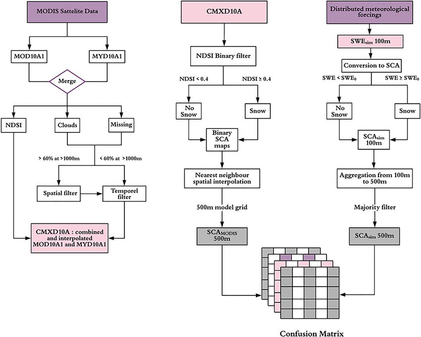
Bouamri et al.                                                                                     Radiation-Induced Snow Cover Spatial Heterogeneity

INTRODUCTION                                                               play a crucial role in determining the spatial variability of
                                                                           snow processes (Lehning et al., 2006; Letsinger and Olyphant,
Snow constitutes a key element in determining water availability           2007; López-Moreno and Stähli, 2008). Interactions between
in mountainous catchments, especially in arid and semiarid                 topography and solar radiation strongly modulates the shortwave
regions, so that a good understanding of snowpack processes is             radiation balance and produce considerable shading effects,
crucial to support water management strategies (Barnett et al.,            especially in high relief landscapes (e.g., Olyphant, 1984).
2005; Viviroli and Weingartner, 2008; De Jong et al., 2009;                While TI models only consider the elevation dependance of
Vicuña et al., 2011; Mankin et al., 2015; Qin et al., 2020). In this       temperature to model the heterogeneity of snowmelt rates,
context, modeling snowmelt and snow water equivalent (SWE)                 adding solar radiation allows to explicitly include the effect of
at the basin scale represents an important tool for water budget           topography on melt and as such to better represent the snow
calculation and runoff prediction (Matin and Bourque, 2013; Bair           cover heterogeneity (e.g., Cazorzi and Dalla Fontana, 1996;
et al., 2016; Fayad et al., 2017; Han et al., 2019).                       Zaramella et al., 2019). Indeed, previous studies have shown
    The lack of ground observations and the large spatiotemporal           that including solar radiation improved the performance of
heterogeneity of snow cover represent challenging limitations              spatially distributed melt models for predictions of glacier
for snow studies in remote mountain ranges (Chaponnière                    mass balance (Gabbi et al., 2014), snow cover area (Cazorzi
et al., 2005; Boudhar et al., 2010, 2016; Rohrer et al., 2013;             and Dalla Fontana, 1996; Follum et al., 2015), and streamflow
Marchane et al., 2015; Collados-Lara et al., 2020). In this context,       from snow-fed basins (Brubaker et al., 1996; Follum et al.,
the use of simple conceptual snow models combined with                     2019; Massmann, 2019). Given the larger computational cost
remote sensing data constitutes a useful approach to assess                entailed to calculate spatially distributed radiation maps,
and quantify snowmelt and SWE distribution at the basin                    it is important to assess their relevance for estimating
scale (e.g., Jain et al., 2010; Abudu et al., 2012; Berezowski             snowmelt with conceptual models aimed for operational
et al., 2015; Dozier et al., 2016; Sproles et al., 2016; Steele            hydrological applications.
et al., 2017; Han et al., 2019). Conceptual models use simplified              Including solar radiation in distributed snowmelt models
process representations with lower data requirements than                  raises the question about the appropriate scale (resolution) to
physically based models, and are thus widely used for large-               run models and the suitability of available data to validate them
scale applications in high mountain catchments where in situ               (Baba et al., 2019). While distributed empirical models can be
observations are sparse (Singh and Bengtsson, 2003; Schneider              run at high spatial resolutions (1000 km2 ), few observations are usually available to validate
conceptual snow models are temperature-index models, which                 spatial simulations explicitly. Snow depth maps from repeat
depend solely on air temperature to calculate snowmelt using the           lidar surveys (Bair et al., 2016; Painter et al., 2016) and satellite
degree-day method (Hock, 2003). Despite their simplicity, these            photogrammetry (Marti et al., 2016) are becoming increasingly
models can provide reliable estimates of melt rates and perform            available, but they remain rare, so that snow cover area (SCA)
generally well both at the point scale and within distributed              maps often represent the sole source of spatially distributed
or lumped hydrological models (Vincent, 2002; Abudu et al.,                snow information to validate distributed snow models. Snow
2012; Kampf and Richer, 2014; Senzeba et al., 2015; Hublart                cover maps derived from the Moderate-Resolution Imaging
et al., 2016; Réveillet et al., 2017). On the other hand, it has           Spectroradiometer (MODIS) sensor onboard the Terra and Aqua
been demonstrated that enhanced temperature-index models                   satellites, available since 2000 and 2002, respectively, have been
that include solar radiation as predictor can outperform classical         at the forefront of distributed snow model calibration and
degree-day models (Cazorzi and Dalla Fontana, 1996; Hock,                  validation efforts (Parajka and Blöschl, 2008; Finger et al., 2011;
1999; Pellicciotti et al., 2005; Carenzo et al., 2009; Homan               Franz and Karsten, 2013; Gascoin et al., 2013; Duethmann
et al., 2011; Carturan et al., 2012; Gabbi et al., 2014; Bouamri           et al., 2014; He et al., 2014; Baba et al., 2018). However,
et al., 2018). This is to be expected, as solar radiation is               its spatial resolution (∼500 m) may often be larger than the
one of the main components of the surface energy balance,                  resolution of key processes, such as topographic radiation loading
generally contributing between 50 and 90% of the energy                    and snow drifting.
available for melt (Willis et al., 2002; Mazurkiewicz et al., 2008),           This paper examines how temperature index snowmelt models
and has a great influence on the spatial variability of ablation           enhanced with different solar radiation components impact the
(Herrero et al., 2009; Aguilar et al., 2010; Comola et al., 2015;          simulated spatiotemporal variability of SWE and snowmelt, and
DeBeer and Pomeroy, 2017).                                                 investigates scaling issues arising when using MODIS snow
    Representing the spatial variability of snow cover within              cover area maps for model validation. We specifically aim to
distributed, parsimonious snowmelt models for hydrological                 show (i) how solar radiation impacts the simulated snowmelt
applications remains challenging, especially in mountainous                dynamics and resulting spatiotemporal heterogeneity in snow
areas where the snow distribution depends on complex                       cover area, and (ii) if and how this heterogeneity is captured
relationships between meteorological conditions and the                    by MODIS snow cover area products that are commonly used
surrounding landscape, primarily topography (Anderton                      for model calibration and validation. This question has not yet
et al., 2004; Molotch et al., 2005; DeBeer and Pomeroy, 2009;              been explored in the snow hydrology community and should thus
Grünewald et al., 2010; Clark et al., 2011). In this sense,                provide further guidance for the implementation and validation
various studies have shown that elevation, slope, and aspect               of distributed empirical snow models.

Frontiers in Earth Science | www.frontiersin.org                       2                                         April 2021 | Volume 9 | Article 640250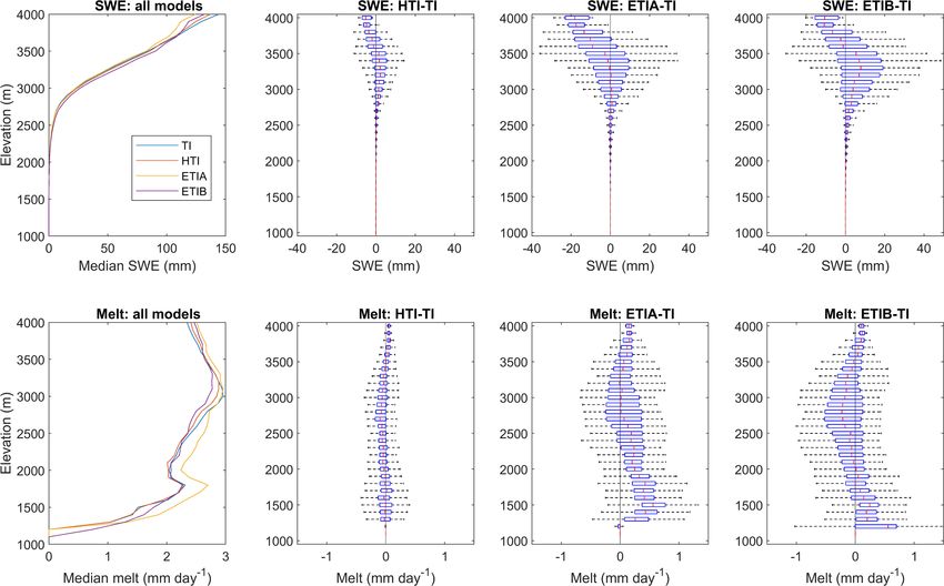
Bouamri et al.                                                                                     Radiation-Induced Snow Cover Spatial Heterogeneity

STUDY AREA                                                                 were excluded to avoid interpolating unreliable observations in
                                                                           winter. The CAF station (2612 m a.s.l.) is thus the only high
The study was carried out in the Rheraya headwater watershed in            elevation station with reliable precipitation observations since
the High Atlas Range in central Morocco (Figure 1). Snowmelt               rainfall and snowfall are independently and manually measured
in this region has important socio-economic implications by                since 1988 (Figure 1).
providing fresh water to irrigate the arid plains downstream,
supplying drinking water for populations and supporting                    Satellite Data
hydropower generation (Chehbouni et al., 2008). The watershed              MODIS Daily Snow Product
covers an area of 228 km2 , and its elevation ranges from 1060             Snow cover maps were derived from the Moderate Resolution
m a.s.l to the Jbel Toubkal summit at 4167 m a.s.l., the highest           Imaging Spectroradiometer (MODIS) daily snow cover products
summit of North Africa. Slopes in the basins are steep (mean of            MOD10A1 and MYD10A1 (MODIS Snow Cover Daily L3 Global
∼24◦ from a 100 m resolution DEM) and characterized by sparse              500 m SIN GRID V006), respectively, generated from the Terra
vegetation in the spring which quickly disappears in summer                and Aqua MODIS satellites, and acquired from the National
due to aridity. The Rheraya watershed has a mixed snow-rain                Snow and Ice Data Center (NSIDC) (Hall and Riggs, 2016). The
regime and constitutes the most important water supply for the             MODIS snow products from the Terra and Aqua satellites are
downstream region (Schulz and de Jong, 2004; Chaponnière et al.,           available since February 2000 and February 2002, respectively.
2005; Rochdane et al., 2012; Hajhouji et al., 2018). Average annual        The datasets are produced in a Geographic projection and
precipitation was 520 mm from 1988 to 2010 as measured at                  were re-projected to the World Geodetic System 1984 (WGS84)
the Club Alpin Francais (CAF) station at 2612 m above sea                  Universal Transverse Mercator (UTM) coordinate system using
level (a.s.l), where 50% occurred as snow during winter months             the data transformation options available at NSIDC. A total of
(Boudhar et al., 2016). The snow cover is highly variable at annual        4734 MOD10A1 images and 4760 MYD10A1 images, covering
and inter-annual time scales and the snowmelt was found to                 13 years from September 2003 to August 2016, were used in
contribute from 28 to 48% of the annual river discharge (Boudhar           this study. Snow cover was identified using the Normalized
et al., 2009). The Rheraya has been used as an experimental                Difference Snow Index (NDSI), which captures the high contrast
site for mountain hydrological studies in the Tensift River basin          between the characteristically high reflectance of snow in the
(Jarlan et al., 2015), leading to a concentration of studies on snow       visible spectrum and its low reflectance in the shortwave infrared
and hydrology in this basin (Boudhar et al., 2016; Baba et al.,            spectrum (Hall et al., 1995). Starting in MODIS version 6, the
2018, 2019; Bouamri et al., 2018; Hajhouji et al., 2018).                  fractional snow cover (FSC) has been replaced by the NDSI which
                                                                           is designed to detect snow cover with high accuracy over a wide
                                                                           range of viewing conditions, besides providing more flexible data
DATA AND METHODS                                                           to the user (Riggs et al., 2015).
The different datasets used in this study are summarized in                Processing and Combining MOD10A1 and MYD10A1
Table 1 and detailed in the following sub-sections.                        Cloud obscuration is the main obstacle to using MODIS snow
                                                                           cover products (Parajka and Blöschl, 2008; Xie et al., 2009;
Digital Elevation Model                                                    Zhou et al., 2013). The Terra and Aqua satellites have an
A 4 m spatial resolution Digital Elevation Model (DEM) derived             approximate 3 h average overpass time difference, during which
from Pleiades stereoscopic imagery was used to represent the               cloud conditions can change significantly (Xue et al., 2014).
basin topography. Details about DEM processing are provided                Various previous studies have shown that combining Terra
in Baba et al. (2019). The DEM was previously validated for the            and Aqua observations reduces cloud obscuration (Parajka and
Rheraya catchment, showing a vertical absolute accuracy of 4.72            Blöschl, 2008; Gafurov and Bárdossy, 2009; Wang and Xie, 2009;
m (Baba et al., 2019). The DEM was aggregated to a coarser 100 m           Xie et al., 2009; Gascoin et al., 2015). For example, Gao et al.
resolution using bilinear resampling. This resolution was chosen           (2010) reported that combining Terra and Aqua improved cloud
as a good tradeoff allowing for a reasonable model computation             filtering by reducing the influence of transient clouds in daily
time while adequately representing the dominant topographic                reflectance data by 11.7% compared to using MOD10A1 alone,
features in the Rheraya catchment (Baba et al., 2019).                     and by 7.7% compared to using MYD10A1 alone. In this study,
                                                                           the MOD10A1 and MYD10A1 were merged into a combined
Meteorological Forcing Data                                                product called CMXD10A (Figure 2) as follow: (i) on any given
Daily meteorological data obtained from ten stations at various            day if only one source (either Terra or Aqua) was available it
locations within or near the Rheraya watershed were used                   was used for that day; (ii) for days when both products are
to distribute meteorological variables to the catchment area               available, priority was given to the Terra product (e.g., Xie et al.,
(Figure 1 and Supplementary Table 1). While precipitation                  2009) since the Aqua MODIS instrument provides less accurate
measurements were available at all ten stations, the availability          snow maps due to dysfunction of band 6 on Aqua (Riggs and
of air temperature and relative humidity varied among stations             Hall, 2004; Salomonson and Appel, 2006; Gascoin et al., 2015;
and over time (Supplementary Figure 1). Two high elevation                 Zhang et al., 2019). This means than any pixel classified as
stations, Oukaimeden-SM (3230 m a.s.l.) and Neltner (3207 m                either cloud, missing, or unclassified in MOD10A1 was filled
a.s.l.) have unheated rain gauges, so their precipitation records          with the corresponding pixel in MYD10A1 if that pixel had a

Frontiers in Earth Science | www.frontiersin.org                       3                                         April 2021 | Volume 9 | Article 640250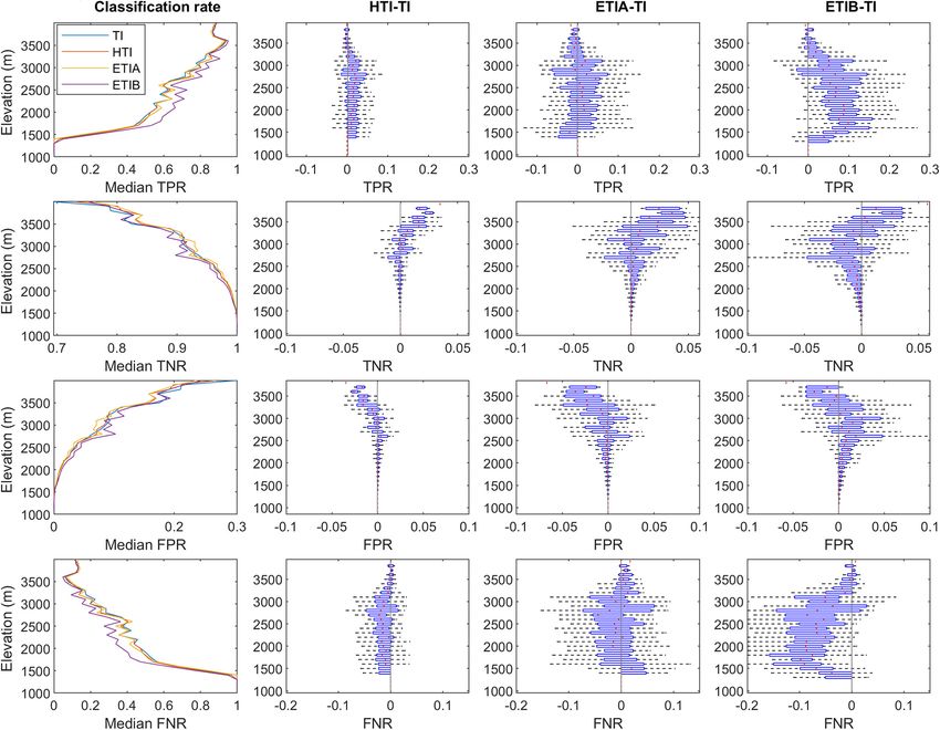
Bouamri et al.                                                                                               Radiation-Induced Snow Cover Spatial Heterogeneity

  FIGURE 1 | Geographical location of the Rheraya basin and weather stations.

TABLE 1 | Data used in the current study.

Data                        Description                         Spatial resolution         Temporal resolution      Time coverage                 Source

MODIS                       MOD10A1 NDSI (0-1)                       ∼500 m                       Daily                2003–2016                  NSIDC
                            MYD10A1 NDSI (0-1)                       ∼500 m                       Daily                2003–2016
DEM                         Pleiades Digital Elevation Model          100 m                         –                       –                Baba et al. (2019)
                            (m)
Meteorological data         Total precipitation (mm)                   Point                      Daily                2003–2016                LMI-TREMA
                            Temperature (◦ C)
                            Relative humidity (%)
SWE                         Reconstructed snow water                   Point                      Daily                2003–2010           Boudhar et al. (2009)
                            equivalent at Oukaimeden (mm)
Model outputs               Snowmelt (mm)                             100 m                       Daily                2003–2016                 This study
                            Snow water equivalent (SWE)
                            (mm)
                            Snow cover area (SCA) (binary)

NDSI value, else the original MOD10A1 pixel classification was                       CMXD10A product were converted to binary maps of snow cover
conserved (Figure 2). Subsequently, a spatiotemporal filter was                      area (SCA) based on an NDSI threshold of 0.4, following previous
applied to the merged CMXD10A product to fill in missing                             studies (Xiao et al., 2004; Marchane et al., 2015; Hall and Riggs,
NDSI data, i.e., pixels classified as cloud, but also those classified               2016), i.e., for each pixel, SCA = 1 when NDSI ≥ 0.4, otherwise
as either missing, saturated or unclassified, collectively referred                  SCA = 0 (Figure 2). The number of pixel identified as missing
to as ‘missing’ therein. A spatial filter was first applied only if                  over the entire period was reduced from 22.35% in MOD10A1 to
less than 60% of the mountainous areas (elevations above 1000                        0.84% after blending both MODIS products and applying cloud
m) were missing (Marchane et al., 2015). This filter classifies                      interpolation, which is similar to previous results obtained in the
missing pixels as being fully snow-covered (NDSI = 1) when                           same area by Marchane et al. (2015).
their elevations is higher than the average elevation of other fully
snow-covered pixels in the entire basin. Then, a temporal filter                     Snowmelt Models
was applied to linearly interpolate the remaining missing pixels                     Four different melt models were used to simulate snowmelt
within a moving window extending 3 days prior and 2 days after                       and SWE in the Rheraya watershed. The benchmark model
the current date. This time window was previously shown to be                        is a classical degree-day or ‘temperature index’ (TI) model
efficient for cloud gap filling by Marchane et al. (2015) in the                     (Hock, 2003), which uses air temperature as the sole predictor
Rheraya catchment. NDSI values in the blended and interpolated                       for melt. This model was ‘enhanced’ with different solar radiation

Frontiers in Earth Science | www.frontiersin.org                                4                                          April 2021 | Volume 9 | Article 640250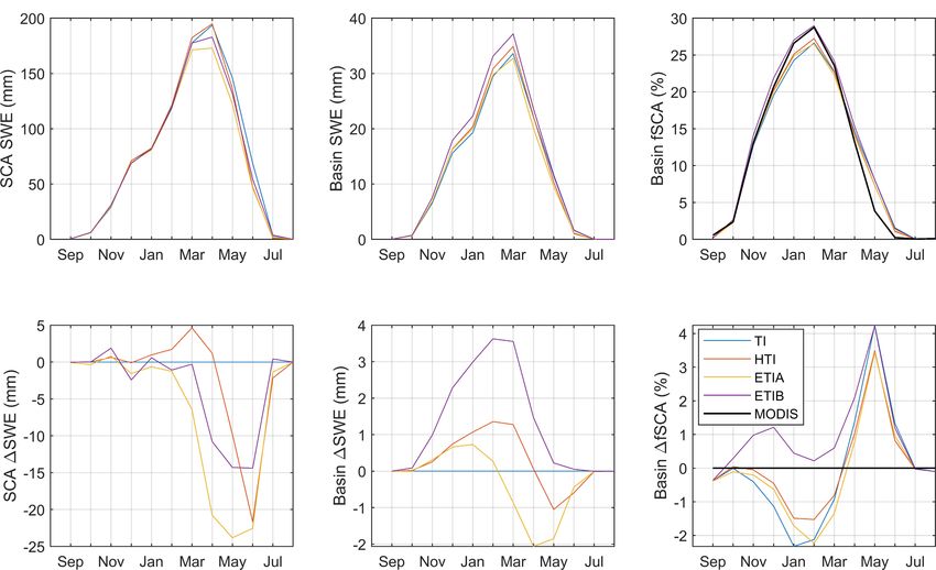
Bouamri et al.                                                                                              Radiation-Induced Snow Cover Spatial Heterogeneity

  FIGURE 2 | Flowchart describing the steps for processing MODIS data and comparing MODIS and simulated snow cover area (SCA). Purple color, data source;
  pink, intermediate output; gray, main output.

terms: (i) Hock’s temperature index melt model (HTI) which                        melt, as can be the case when sublimation losses are
includes clear sky potential solar radiation (Hock, 1999); (ii) an                completely ignored.
enhanced temperature-index (ETIA) including global radiation
and (iii) an enhanced temperature-index (ETIB) that includes                      Rain/Snow Partition
albedo (Pellicciotti et al., 2005; Table 2). These models were                    Determination of the precipitation phase has a large influence
previously calibrated and validated at the point scale at the                     on hydrological modeling in mountain areas (Yasutomi et al.,
Oukaimeden-SM weather station site (Bouamri et al., 2018), and                    2011; Marks et al., 2013). A linear transition technique was used
the same model coefficients were used for the spatial simulations                 for the rain-snow partition (e.g., Marks et al., 2013; Feiccabrino
in this study (Table 3). Further model descriptions and results                   et al., 2015). The snowfall fraction is linearly interpolated between
regarding model performances at the point scale are presented                     a temperature threshold for rain Train (◦ C), and a temperature
in detail in Bouamri et al. (2018), and only the main model                       threshold for snow Tsnow (◦ C) (Tarboton and Luce, 1996; Moore
equations are given in Table 2.                                                   et al., 2012). The daily snowfall (SF) and rainfall (RF) are
    Sublimation losses are not accounted for in empirical                         computed as:
melt models. These can be significant in the Rheraya basin,
representing 7–20 % of annual snowfall (Boudhar et al.,                                          SF = Px (Train − Tx ) / (Train − Tsnow )                   (1a)
2016). To take into account sublimation losses, a constant
average mean daily sublimation rates was used over the                                                         RF = Px − SF                                 (1b)
entire basin (Table 3), based on the energy balance study
at the Oukaimeden-SM site by Boudhar et al. (2016). While                            Where Px is total precipitation and Tx is air temperature
this approach is admittedly simple, it allows correcting for                      at gridpoint x. If the daily air temperature is above the Train
first order sublimation losses (Jost et al., 2012) and as                         threshold then RF = Px and SF = 0, while if Tx < Tsnow then
such avoid compensating these losses by artificially reducing                     RF = 0 and SF = Px . The two fixed temperature thresholds,
precipitation during spatial interpolation and/or overestimating                  Train and Tsnow , were calibrated on odd years and validated

Frontiers in Earth Science | www.frontiersin.org                              5                                            April 2021 | Volume 9 | Article 640250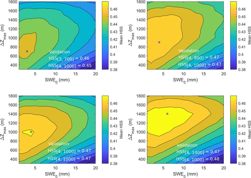
Bouamri et al.                                                                                         Radiation-Induced Snow Cover Spatial Heterogeneity

on even years using independant observations of snowfall and              TABLE 2 | Melt models equations used in this study.
rainfall available at the CAF station over 2003–2016. Optimal
                                                                          Snowmelt models                                     Equations
values for Tsnow and Train were -2.5 ◦ C and 2.5 ◦ C, respectively.
The agreement between simulated and measured precipitation                Classical temperature                           (
                                                                                                                              DDF × Ta    Ta > TT
was fair for rainfall, with a Nash-Sutcliffe Efficiency score (NSE)       index (TI) melt model                     M=                                         (3)
                                                                                                                                   0      Ta ≤ TT
(Nash and Sutcliffe, 1970) of 0.54 and correlation coefficient
                                                                          Hock’s temperature
                                                                                                                    (
(r) of 0.75, and better for snowfall (NSE = 0.77, r = 0.88)                                                             (MF + RF×Ipot )Ta    Ta > TT
                                                                          index melt model (HTI)             M=                                               (4a)
(Supplementary Figure 3). The better performance for snowfall                                                                      0         Ta ≤ TT
is encouraging for the ensuing SWE modeling.
                                                                                                             Ipot = I0 (Dm /D) × ψa(P/P0 cos Z) × cos θ       (4b)

Spatialization of Meteorological Forcing                                  Enhanced
                                                                                                               (
                                                                                                                   TF × Ta + SRFin × I      Ta > TT
Half-hourly meteorological observations retrieved from the                temperature-index               M=                                                  (5a)
                                                                                                                               0            Ta ≤ TT
different weather stations were averaged to daily interval for the        (ETIA) melt model
entire study period (2003–2016). Relative humidity (RH) was                                               R = −0.000054 × RH2 − 0.0024 × RH + 1.3 (5b)
converted to dew point temperature (DP) following Liston and                                              I = R × Ipot                                        (5c)
Elder (2006), since RH is considered a non-linear function of
elevation. Mean monthly lapse rates (i.e., averaged over the whole        Enhanced
                                                                                                                (
                                                                                                                    TF × Ta + SRFnet (1 − α)I       Ta > TT
period) were determined by linear regression of air temperature           temperature-index               M=
                                                                                                                                   0                Ta ≤ TT
                                                                                                                                                              (6a)
(Ta) and DP against elevation. Since the seasonal variability in          (ETIB) melt model
the lapse rates was small, a mean annual value was used in the                                            α = p1 − p2 (log10 (PDD))                           (6b)

models (Table 3). To distribute Ta and DP observations, station           Variables are defined in footnote -| and model parameters in Table 3 -| M is the
observations were first adjusted to a common elevation using              melt rate (mm d−1 ), Ta is daily mean air temperature (◦ C) and TT is a threshold
the calculated lapse rate for each variable, and then spatially           temperature fixed at 0◦ C. Ipot is the potential clear-sky incoming direct solar
interpolated to the entire basin using the Barnes objective               radiation (W m−2 ), I0 is the solar constant (1368 W m−2 ), Dm and D are the
                                                                          mean and actual Sun-Earth distance, ψa is the vertical clear-sky atmospheric
analysis scheme, following Liston and Elder (2006). The Barnes            transmissivity (0.75), P is the atmospheric pressure in Pa and P0 is standard
scheme is used for interpolating data from irregularly spaced             atmospheric pressure (101 325 Pa). Z is the solar zenith angle, and θ is the
observations to a regular grid using a two-pass scheme (Barnes,           incidence angle of the Sun on the surface. I is incoming shortwave radiation (W
                                                                          m−2 ), R is the ratio between the incoming shortwave radiation (I) and the potential
1964). The interpolated values are then lapsed back to their              clear-sky direct solar radiation (Ipot ).α is snow albedo, where PDD (mm ◦ C−1 d−1 )
original grid elevation using the same lapse rate, and the DP             is the positive degree-day sum since the last snowfall. The parameter p1 represents
reconverted to RH.                                                        a typical maximum albedo value for fresh snow (0.8) and p2 is the empirical snow
   Precipitation was spatially distributed by combining spatial           albedo decay parameter (0.21). RH is relative humidity.

interpolation with a non-linear lapse rate, following Liston and
Elder (2006). First, precipitation observations are interpolated
to the model grid using the Barnes objective analysis scheme.             (2007–2008, 2009–2010) (Supplementary Figure 2). The optimal
A reference topographic surface is constructed by interpolating           value found, 0.35 km−1 , was used to distribute precipitation
the station true elevations (as measured by GPS) using the same           using equation (2).
method. The modeled precipitation rate Px (mm d−1 ), at a grid               The extrapolation of precipitation using equation (2) can
point x with elevation Zx is computed as:                                 result in unrealistically large accumulation rates at high elevations
                                    [1 + PLR (Zx − Z0 )]                  where there are few stations to constrain precipitation. Several
                     Px = P0 ×                                 (2)        studies have shown that while precipitation typically increases
                                    [1 − PLR (Zx − Z0 )]
                                                                          with elevation in mountain basins due to orographic uplifting
   Where P0 is the interpolated station precipitation, Z0 is              of air masses, this increase can cease and precipitation even
the interpolated station elevation, and PLR (mm km−1 ) is the             decrease passed a certain elevation (Alpert, 1986; Roe and Baker,
precipitation lapse rate, or ‘correction factor’ (Liston and Elder,       2006; Eeckman et al., 2017; Collados-Lara et al., 2018). This is
2006). An interpolated topographic reference surface (Zx ) is used        caused by the progressive depletion of moisture available for
rather than a fixed reference because the precipitation adjustment        condensation within the rising air mass. As such, it is crucial
function (equation (2)) is a non-linear function of elevation             in hydrological modeling to limit the vertical extrapolation
(Liston and Elder, 2006).                                                 of precipitation to avoid artificial snow build up at high
   Due to the large spatial and temporal heterogeneity of                 elevations (Freudiger et al., 2017). In this sense, Liston and
observed precipitation in Rheraya, a specific calibration of PLR          Elder (2006) limited the difference between the actual (Zx )
was sought. A range of 0.21- 0.35 km−1 was used based on the              and interpolated (Z0 ) station elevation (4Z = Zx − Z0 ) to a
lapse rate value fitted to station observations and the typical           default maximum value (4Zmax ) of 1800 m. Since there are no
winter value set by Liston and Elder (2006) and also found by             stations with reliable precipitation data above the CAF station
Baba et al. (2019) in the Rheraya basin. The PLR was calibrated           (2612 m) to constrain this value, this parameter was subjected
against positive SWE changes at the Oukaimeden-SM station,                to a calibration/validation procedure against the MODIS SCA
a proxy for snow accumulation, over a lumped 3-year period                maps for all melt models. 4Zmax was calibrated on odd years
(2003-2006) and validated separately on the remaining 2 years             within a 300-1800 m range and validated on even years for

Frontiers in Earth Science | www.frontiersin.org                      6                                                   April 2021 | Volume 9 | Article 640250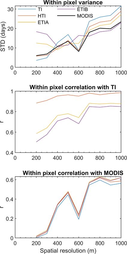
Bouamri et al.                                                                                                       Radiation-Induced Snow Cover Spatial Heterogeneity

TABLE 3 | Summary of prescribed and calibrated model parameters.

Prescribed           Description                       Optimal value         Unit                  Calibrated                Description              Optimum          Unit
parameter1                                                                                         parameter                                           value

DDF                  Degree-day factor                      2.7         mm d−1 ◦ C−1                   TLP              Temperature lapse rate          −0.56    ◦C    100 m−1
MF                   Melt factor                            1.8         mm   d−1 ◦ C−1                DPLR               Dew point lapse rate           −0.68    ◦C    100 m−1
RF                   Potential radiation factor            0.005   m2 mm W−1 d−1 ◦ C−1                 PLR              Precipitation lapse rate         0.35          km−1
TFA                  Temperature factor ETIA                1.1         mm d−1 ◦ C−1                  SWE0               SWE-SCA threshold                 4           mm
SRFin                Incoming shortwave radiation factor   0.025       m2 mm W−1 d−1                 4Z max         Maximum elevation difference        1000            m
TFB                  Temperature factor ETIB                0.6         mm d−1 ◦ C−1                  Tsnow        Temperature threshold for snow        −2.5           ◦C

SRFnet               Net shortwave radiation factor        0.07        m2 mm W−1 d−1                   Train        Temperature threshold for rain        2.5           ◦C

p1                   Fresh snow albedo                      0.8                –
p2                   Albedo decay parameter                0.21                –
Subli                Sublimation rate                      0.244          mm d−1
1 From   Bouamri et al. (2018).

each model in order to reduce the climate dependency of                                relative to that expected by chance and has been extensively
the calibration period (Arsenault et al., 2018). The validation                        used for imbalanced datasets such as snow remote-sensing data
was done using the optimal parameter for each model as                                 (e.g., Zappa, 2008; Notarnicola et al., 2013; Baba et al., 2019).
well as with the mean of the optimal parameters of each                                The HSS was thus the preferred global metrics used for model
model (mean 4 Zmax ).                                                                  assessment. Still, because no global metric is able to completely
   The potential, clear-sky direct solar radiation was calculated                      depict the types of classification errors committed by a model,
as a function of solar geometry, topography and a constant                             four metrics based on marginal ratios of the confusion matrix
vertical atmospheric transmissivity following Hock (1999), and                         were also used to investigate model errors, as done in several
includes topographic shading (Equation 4b in Table 2). Global                          previous studies (e.g., Parajka and Blöschl, 2012; Rittger et al.,
radiation is calculated using a cloud factor parameterization                          2013; Zhou et al., 2013; Zhang et al., 2019). The true positive
based on relative humidity (Bouamri et al., 2018) (Equation 5b, c                      rate (TPR) measures the proportion of MODIS snow-covered
in Table 2) and the net radiation uses an albedo parameterisation                      pixels correctly identified as such by the model. Oppositely, the
based on accumulated positive degree days (Brock et al.,                               true negative rate (TNR) measures the proportion of MODIS
2000) (Equation 6b in Table 2). Further details are given in                           snow-free pixels correctly simulated by the model. The false-
Bouamri et al. (2018).                                                                 negative rate (FNR) measures the proportion of MODIS snow-
                                                                                       covered pixels incorrectly identified as snow-free by the model.
Model Validation                                                                       Complementarily, the false-positive rate (FPR) or ‘False Alarm
The daily snow cover area (SCA) from the merged CMXD10A                                Rate’ (FAR) as called by Zappa (2008) is the proportion of
product was used to assess the ability of each model to simulate                       MODIS snow-free pixels incorrectly identified as snow-covered
the spatiotemporal variability of snow cover in the Rheraya                            by the model. Further descriptions of theses metrics are given
basin over the 2013-2016 period. A conversion of the simulated                         in Table 4.
SWE to SCA was required to compare the simulated SCA
with MODIS SCA. This conversion was performed using a
constant threshold (SWE0 ), i.e., for each grid, SCA = 1 when
SWE ≥ SWE0 and SCA = 0 otherwise. The conversion was                                   TABLE 4 | Description of confusion matrix between simulated and MODIS SCA,
done at the model resolution (100 m). The use of this fixed                            and the evaluation metrics used for model assessment.
threshold avoids more complex snow depletion curves that
                                                                                                                                           SCA MODIS
require more parameters unknown in our area (Magand et al.,
2014; Pimentel et al., 2017). Therefore, SWE0 was subjected to the                     SCAsim                         Snow                                Snow free
same calibration/validation procedure as for4Zmax , using a range
of values from 1 to 20 mm following previous studies (Gascoin                          Snow                             TP                                      FP

et al., 2015; Baba et al., 2019).                                                      Snow free                        FN                                      TN

    Confusion matrices were used to assess the classification                          Metrics                                              Definitions
accuracy of the simulated SCA maps relative to MODIS SCA.
Confusion matrices are two-dimensional contingency tables that                         TPR                                                 TP/(TP + FN)

display the discrete joint distribution of simulated and observed                      TNR                                                 TN/(TN + FP)
                                                                                       FNR                                                 FN/(FN + TP)
data frequencies (Zappa, 2008). Model skill scores were derived
                                                                                       FPR                                                  FP/(F + TN)
from the confusion matrix (Table 4). The Heidke Skill Score                                                                              2×(TP×TN−FP×FN)
                                                                                       HSS
(HSS) (Heidke, 1926) which is equivalent to the Kappa coefficient                                                                (TP+FP)×(FP+TN)+(TP+FN)×(FN+TN)

proposed by Cohen (1960), measures the classification accuracy                         TP, true positive; TN, true negative; FP, false positive; FN, false negative.

Frontiers in Earth Science | www.frontiersin.org                                   7                                                  April 2021 | Volume 9 | Article 640250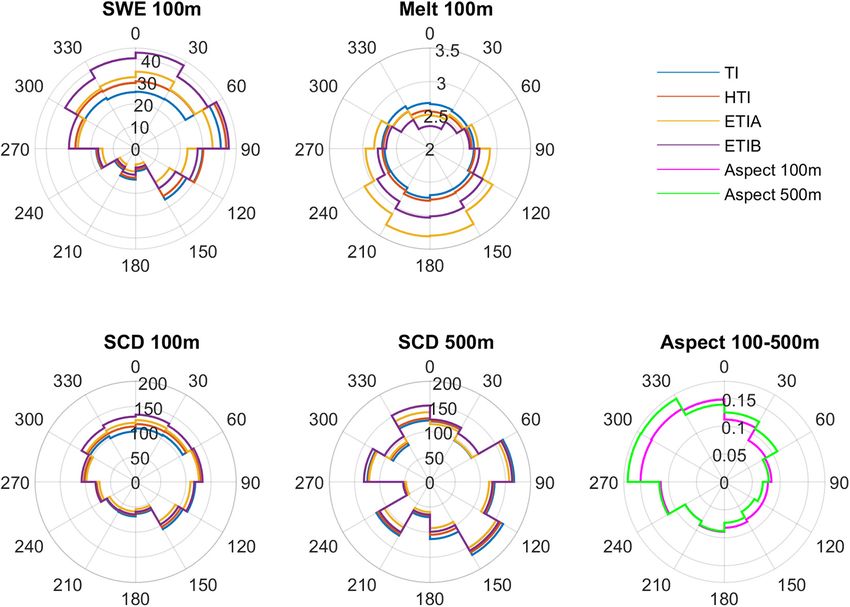
Bouamri et al. Radiation-Induced Snow Cover Spatial Heterogeneity
RESULTS scarce snowfall and thinner simulated snowpack (e.g., 2011,
2013, 2014, and 2016), the agreement between simulated and
Basin-Wide Snow Cover Area observed fSCA is better (Figure 4D). The varying availability
Parameter Sensitivity and Calibration of precipitation records over time could also partly explain this
The sensitivity of SCA model performance to the maximum pattern (Supplementary Figure 1).
elevation difference (4Zmax ) and SWE-SCA conversion All four models show slight differences in their basin-wide
threshold (SWE0 ) was assessed using the mean daily HSS metric fSCA and SWE predictions. Error metrics for the whole period
computed over the calibration period, i.e., the odd years of the (2003-2016) show that increasing model complexity slightly
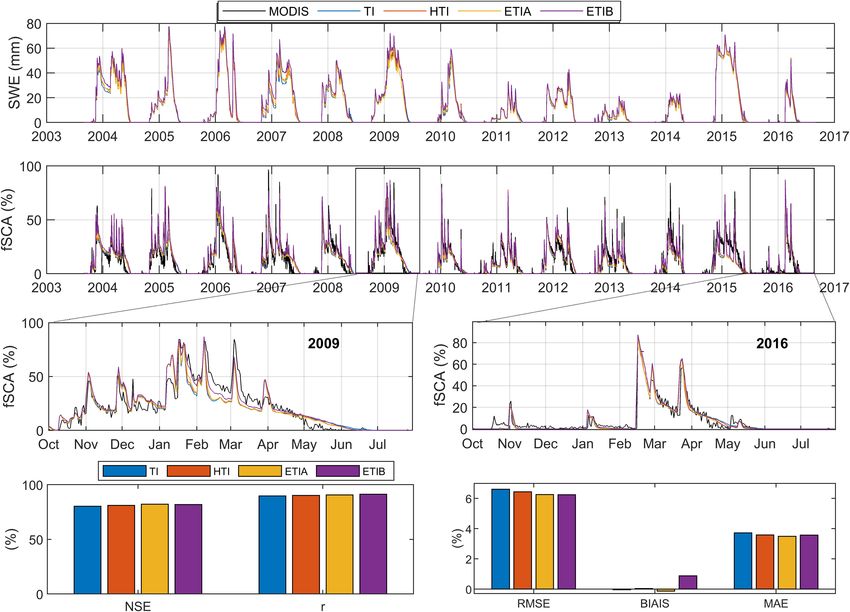
2003-2016 period (Figure 3). Generally, the model performance improves the correlation (r) and predictive skill (NSE) for basin-
increases with model complexity, i.e., the HSS is lowest for TI wide fSCA (Figure 4E). Both the root mean squared error
and highest for ETIB. All four models are more sensitive to (RMSE) and mean absolute error (MAE) also decrease with
4Zmax than the SWE0 parameter. The mean optimal SWE0 varies model complexity, but a larger bias for the ETIB model slightly
between 3 mm for TI to 6 mm for ETIB, with little variations in increases its MAE relative to the ETIA model (Figure 4F). Hence,
HSS score within this range as well as within each model. A mean overall, the best performance is primarily observed for both
optimal SWE0 value of 4 mm was thus used for validation enhanced radiative models ETIA and ETIB followed by the HTI
on even years and for further inter-model comparisons. This and the classical TI models. Still, given the slight differences
value is small compared to the 40 mm threshold used by Baba between models and the increased computational cost associated
et al. (2019) and Gascoin et al. (2015) but SWE0 is resolution with enhanced radiative models, the TI model offers at first glance
dependent, increasing with pixel resolution (Gascoin et al., a satisfactory performance to simulate SWE for hydrological
2019). The optimal 4Zmax shows more variability between applications in the High Atlas range. The causes for inter-model
models, increasing with model complexity, i.e., lowest for TI differences in model performance and in simulated SWE and
and highest for ETIB. This is in fact to be expected from this melt are explored in the next sections.
parameter, which should also partly correct errors in modeled
ablation. Using a common 4Zmax and SWE0 value avoids the Seasonality
problem of compensating snowmelt parameterisation errors in The seasonality of the simulated SWE and fSCA was investigated
each model, which would prevent any further direct comparison to better understand seasonal inter-model differences
of the snowmelt parameterisations. A mean 4Zmax of 1000 m, (Figures 5A–C). The enhanced models were then contrasted
which is within the zone of maximum performance for each with the reference TI model to highlight the effect of the different
model (Figure 3) was thus used for validation across models and radiation terms on the simulated snow cover (Figures 5D,E). The
for further inter-model comparisons. Choosing the multi-model mean basin SWE seasonal cycle calculated over snow-covered
average parameter set (SWE0 = 4 mm, 4Zmax 1000 m) over the areas (‘SCA SWE’) shows similar variations among models,
model-specific optimal parameters affects little the performance particularly during the accumulation season (October-March)
in validation (Figure 3). In fact, a slight increase in performance (Figure 5A). The mean simulated peak occurs in April and varies
is even noted for ETIB, which suggests that the model-specific from 172 mm to 195 mm between models. Increasing differences
values may be slightly overfitted and less transferable compared between the ETI models and TI from March to May reflect the
to the multi-model average parameter set. increasing ablation rates simulated by these models relative to TI,
The slight overall differences in performance between models while the HTI model differs significantly from TI only from May
suggest that, on average, all models have similar abilities to onward when the SCA is low (Figure 5D). Maximum differences
classify snow vs. snow free MODIS pixels, as assessed by the mean with TI are reached at peak SWE in April for ETIA (-24 mm)
HSS metric. The small differences could be partly attributed to and ETIB (-14 mm) and in June for HTI (-21 mm) (Figure 5D).
the fact that performance metrics are averaged over the whole The ETIA model, which does not include albedo feedbacks, thus
calibration period. Hence, interannual and seasonal differences tends to accentuate most the melt rates in early spring compared
in model performance are investigated next. to TI. The melt coefficients of ETIA, previously calibrated at the
Oukaimeden station, may be slightly biased towards late spring
conditions, which results in exaggerated late-winter/early spring
Basin-Wide SWE and SCA melt rates (Bouamri et al., 2018).
Time series of daily simulated basin wide SWE and fractional When considering mean SWE over the whole basin surface
snow cover (fSCA) show significant intra and inter-annual (“Basin SWE”), differences between the enhanced models and
variability over the period (2003-2016) (Figure 4). The fSCA TI are more positive during winter and occur at different times
simulated by the four models are in good agreement overall with (Figure 5B). ETIB stands out with the largest mean peak SWE
MODIS observations, both in terms of timing and magnitude. of 37 mm in March, followed by HTI and the other models. In
In some years, however, the simulated snow cover lasts longer contrast to the classical TI model, all radiative models simulate
than observed in MODIS (2004, 2005, 2007, 2008, 2009, and higher mean basin SWE during the accumulation period, while
2012). Those years had above average basin-wide simulated SWE ETIA and HTI simulate lower SWE in late spring compared to TI.
(Figure 4A), so that overestimated accumulation in the upper The different seasonal behaviors for the mean basin SWE
basin during these wetter years could be the cause for the longer- and mean SWE over snow covered areas can be explained
lasting simulated SCA (Figure 4C). In contrast, in years with by differences in simulated SCA. All models, except ETIB,
Frontiers in Earth Science | www.frontiersin.org 8 April 2021 | Volume 9 | Article 640250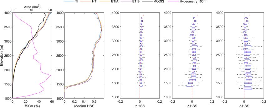
Bouamri et al.                                                                                                    Radiation-Induced Snow Cover Spatial Heterogeneity

  FIGURE 3 | Sensitivity of model SCA simulation performance, as assessed with the mean HSS index, to 4Z max and SWE 0 parameters over the calibration period.
  Optimal parameter values are indicated by asterisks (*). The validation HSS statistics for the model-specific and multi-model average optimal parameters are shown
  in white. (A) TI, (B) HTI, (C) ETIA, and (D) ETIB.

underestimated MODIS fSCA during accumulation, whereas                                (Figure 7). Overall, the HSS index increases with elevation for
all models overestimated MODIS fSCA on average during the                             all models (Figure 7B). The mean simulated fractional snow
ablation period, by up to 4.2% for ETIB and TI, and by 3.4%                           cover area (fSCA) also increases with elevation, in line with
for HTI and ETIA (Figures 5C,F). This confirms the tendency                           MODIS fSCA, but all models start overestimating fSCA above
identified in Figure 4 for wet years to have a longer-lasting snow                    3500 m (Figure 7A). The worst model performance (lowest
cover simulated by all models, relative to MODIS. Inter-model                         HSS) are thus associated with the marginal and transient snow
differences show that all enhanced models simulate a larger snow                      conditions found at the lowest elevations of the basin. Since these
cover than TI during the accumulation period, with ETIB being                         elevation areas represent a large share of the basin hypsometry
the most different and also most in line with MODIS, followed                         (Figure 7A), the higher classification errors in these areas have a
by HTI and ETIA. This explains the positive differences in basin                      large influence on the basin-wide and time-averaged performance
SWE between these models and TI during the accumulation                               metrics, as displayed on Figure 3.
period (Figures 5B,E).                                                                    All enhanced models perform generally better than TI,
    Seasonal variations in SCA model performance, as measured                         although the gains in performance remain overall small
by the HSS index, were investigated over the whole period                             (Figures 7C–E). Elevation trends also differ between the radiative
(Figure 6). Globally, the HSS metric is highest (∼0.6-0.75) during                    models. ETIB performs best, but the improvement is most
winter and spring (December-April) but decreases sharply during                       pronounced at lower elevations (Z < 3000m), which represent
the shoulder seasons (October to November and May to June).                           a large portion of the total basin but where there is less snow
This shows that the model performance is generally good during                        present throughout the year (Figure 7A). At high elevations
most of the snow season, but that classification errors increase                      (Z > 3000m) where mean SCA is above 30%, the gain in
when the snow cover is more restricted in the basin. All radiative                    performance becomes more marginal for ETIB, while it is
models performed better than TI especially in the accumulation                        somewhat more pronounced for HTI and ETIA. While the
period, with ETIB performing best, with a maximum increase in                         bulk of the elevation bands show increased performance of the
HSS of 0.03. The models become gradually more similar in late                         radiative models relative to TI, a small portion of grid points, in
spring (May-June).                                                                    some cases up to ∼20% (left side of boxes in Figure 7 boxplots),
                                                                                      actually suffer increased errors relative to TI.
Spatial Variability                                                                       Further insights into the performance behavior between
Model performance in predicting spatial variations in SCA                             models can be obtained by looking at classification success (TPR,
was investigated by plotting the HSS metric by elevation bins                         TNR) and error rates (FPR, FNR) by elevation (Figure 8).

Frontiers in Earth Science | www.frontiersin.org                                  9                                              April 2021 | Volume 9 | Article 640250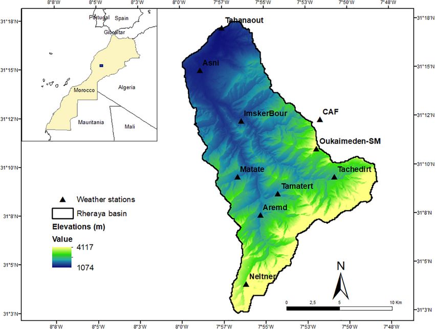
Bouamri et al.                                                                                                Radiation-Induced Snow Cover Spatial Heterogeneity

  FIGURE 4 | Time series of (A) simulated mean snow water equivalent (SWE), and (B) simulated mean fractional snow cover area (fSCA) of all models vs. MODIS;
  (C) zoom in on 2009 year; (D) zoom in on year 2016; (E,F) errors statistics over the entire period 2003–2016 in the Rheraya catchment.

  FIGURE 5 | Seasonal cycle of mean simulated snow water equivalent (SWE). (A) Over snow-covered area only. (B) Over the whole basin. (C) Mean simulated fSCA
  vs. MODIS. (D,E) Difference between radiative models and the reference TI model for panels A and B. (F) Difference between modeled and MODIS fSCA.

Frontiers in Earth Science | www.frontiersin.org                               10                                            April 2021 | Volume 9 | Article 640250
Bouamri et al.                                                                                                  Radiation-Induced Snow Cover Spatial Heterogeneity

                                                                                      the more transient snow zone (∼1500–3200m), with ETIB clearly
                                                                                      performing best. The improvement for HTI is small but rather
                                                                                      consistent with altitude, whereas ETIA shows more variations
                                                                                      with even losses in performance in the highest and lowest
                                                                                      altitudes relative to TI. Opposite to TPR, the true negative rate
                                                                                      (TNR) decreases with altitude. Both ETI models show the largest
                                                                                      deviations with TI, but with decreased accuracy at medium
                                                                                      elevations, especially for ETIB (Figure 8: row 2). The elevation
                                                                                      profile of the false positive error rate (FPR) shows that all models
                                                                                      tend to over predict snow presence towards higher altitudes
                                                                                      (Figure 8: rows 3). Conversely, models rarely overpredict snow-
                                                                                      free conditions at high elevations but do so at the lower elevations
                                                                                      (Figure 8: rows 4). The enhanced models can be seen to reduce
                                                                                      both the FPR and FNR errors on average, but large scatter occurs
                                                                                      within elevation bands. The clearer improvement relative to TI is
                                                                                      the decreased FNR error for ETIB (Figure 8D: rows 4).
                                                                                          Despite the overall good performance for the simple TI model,
                                                                                      the enhanced models, especially ETIB, still explained more
                                                                                      variability in SCA within most elevation bands, but with notable
                                                                                      discrepancies among models (Figure 7). To better understand
                                                                                      these discrepancies, the simulated SWE and melt rates were
                                                                                      compared by elevation band (Figure 9). The HTI model shows
                                                                                      the smallest difference relative to TI, in line with its more
                                                                                      similar performance in SCA simulations. This can be attributed
                                                                                      to the fact that HTI only adjusts the degree-day factor based
                                                                                      on the potential clear-sky radiation and thus ignores temporal
                                                                                      variations in atmospheric transmissivity and albedo. On the other
                                                                                      hand, both ETI models show significant differences in simulated
                                                                                      SWE (Figures 9C,D) and melt rates (Figures 9G,H) relative
                                                                                      to TI. The best performing ETIB model simulates smaller melt
  FIGURE 6 | Seasonal model performance. (A) Mean seasonal cycle of HSS               rates and larger SWE at middle elevations (2000–3500 m), and
  index over the whole 2003–2016 period. (B) Differences between enhanced             higher melt rates and smaller SWE at the highest elevations
  radiative models and the reference temperature index (TI) model.                    (>3500 m). Interestingly, the median differences in SWE and
                                                                                      melt rates between the enhanced models and TI per elevation
                                                                                      band are rather small, which again shows that the preponderant
Overall, the true positive rate (TPR) increases with elevation,                       influence of elevation on the simulated SWE is well captured
reaching a maximum value of ∼0.9 around 3600 m (Figure 8: row                         by the simple TI model. However, significant deviations occur,
1). The enhanced models better classify snow presence than TI in                      up to ca. ± 20 mm for SWE and ca. ± 1 mm d−1 for

  FIGURE 7 | Model validation and intercomparison by elevation. (A) Distribution of mean fSCA per elevation range and basin hypsometry. (B) Median HSS index of all
  models by elevation. (C–E) HSS differences between radiative and reference TI model by elevation range: (C) HTI. (D) ETIA. (E) ETIB.

Frontiers in Earth Science | www.frontiersin.org                                 11                                            April 2021 | Volume 9 | Article 640250
Bouamri et al. Radiation-Induced Snow Cover Spatial Heterogeneity
FIGURE 8 | SCA classification errors by elevation; 1st row, true positive rate (TPR); 2nd row, true negative rate (TNR); 3rd row, false positive rate (FPR); 4th row, false
negative rate. (A) Median error rate. (B–D) Differences between radiative and classical TI model.
melt rates (Figures 9C,D,G,H). Given that the simulated SWE southern slopes (Figures 10A,B), which results in longer-lasting
diverges most between models from March onto the melt season snow on northern slopes compared to the TI model (Figure 10C).
(Figure 5), it is intriguing that these significant differences in melt Aggregation of the simulated SCA from 100 m to 500 m results
rates and SWE do not result in larger inter-model differences in significant disruption of this pattern (Figure 10D), which can
in simulated SCA and more so between the simulated SCA and be attributed to changes in the distribution of slopes and aspects
MODIS SCA (Figure 7). This suggests that these differences in following aggregation (Figure 10E).
the spatial heterogeneity of melt rates between models may not To better constrain the influence of scaling effects on
be adequately captured by the pixel resolution of MODIS snow the simulated SCD at 100 m resolution and its relationship
cover maps, a topic explored in the next section. with MODIS, the subgrid variability (standard deviation) was
calculated for different pixel aggregation scales, from 200 m up
to 1000 m (Figure 11A). Both ETI enhanced models clearly show
Effect of Spatial Resolution on SCA higher subgrid variability than the TI model at scales below ∼400
Validation m, due to pronounced topographic-induced variability in solar
In order to compare the simulated SCA with MODIS, the radiation at those scales. The ETIB model, which includes albedo,
modeled SCA was aggregated from 100 m to the 500 m resolution shows the highest subgrid variability. The subgrid variability of
of MODIS (Figure 2). This has the potential to suppress MODIS (here resampled at 100 m) is expectedly low below its
significant spatial variability in the finer (100 m) scale simulated nominal resolution (500 m) and similar to that simulated by
SCA. To explore this further, the mean snow cover duration the TI and HTI models. At large aggregation scales (>400 m)
(SCD = mean SCA × 365 days) simulated at the original 100 m elevation effects begin to dominate and the TI model displays
resolution was compared to that aggregated at the MODIS 500 m more subgrid variability than the enhanced models, while the
resolution by aspect (Figure 10). The smoothing effect of model ETIB subgrid variability is most in line with MODIS. The
aggregation is particularly evident: at the original 100 m model influence of the aggregation scale on model intercomparison is
resolution, all radiative models expectedly simulate smaller melt seen in Figure 11B: the subgrid correlation between the enhanced
rates and larger SWE on northern slopes, and vice-versa on models and the reference TI model decreases at scales below 700
Frontiers in Earth Science | www.frontiersin.org 12 April 2021 | Volume 9 | Article 640250Bouamri et al. Radiation-Induced Snow Cover Spatial Heterogeneity
FIGURE 9 | Mean simulated SWE and melt by elevation for days with snow. (A) Median SWE for all models. (B–D) SWE differences between radiative and reference
TI model. (E) Median melt rate for all models. (F–H) Melt differences between radiative and TI model.
m and show that the enhanced models are most different from MODIS snow cover maps, their significant extra computational
TI below 400 m. However, the subgrid correlations between the cost implies that the simpler TI would be adequate for operational
simulated SCD and MODIS SCD show little differences between snow simulations in this basin. This contrasts with previous
models, because MODIS does not sample the spatial variability studies that showed that including solar radiation improves the
below 500 m (Figure 11C). Hence, the consideration of global performance of spatially distributed melt models for predictions
(ETIA) and net (ETIB) solar radiation introduces significant of glacier mass balance (Gabbi et al., 2014), snow cover area
variability in SCD at scales not sampled by MODIS. (Cazorzi and Dalla Fontana, 1996; Follum et al., 2015), and
streamflow from snow-fed basins (Brubaker et al., 1996; Follum
et al., 2019). On the other hand, the use of a fully distributed
DISCUSSION AND CONCLUSION (grid-based) model improved the simulations of SCA relative to
semi-distributed temperature index models previously applied in
Difference in Model Performance this basin (Boudhar et al., 2009).
The enhanced radiative models, especially ETIB, showed The increasing false positive error rate (FPR) and decreasing
increased performance relative to the simplest TI model for false negative error rate (FNR) with elevation suggest that
predicting basin wide SCA over time (Figure 4). In particular, there may be a persistent elevation bias in the simulated
the peak SCA in February was notably better simulated by SCA (Figure 8), which is partly alleviated by the radiative
the ETIB model compared to the other models (Figure 5C). models, in particular ETIB. This suggests that increasing global
However, overall differences in model performance were small. radiation with altitude due to higher atmospheric transmissivity
Our results show that most of the snow cover variability is and the consideration of snow albedo result in steeper
driven by elevation and that this trend was adequately captured ablation profiles compared to temperature-only melt calculations
by all four models (Figure 7). Hence the simple TI model with the TI model.
could be considered sufficient for melt simulations at the basin The effect of model parameters uncertainties must also be
scale, due to the strong dependence of temperature and related considered. The remaining elevation trends in the error rates in
melt rates on elevation, as found elsewhere (e.g., Vincent, 2002; Figure 8 point to lingering problems with the distribution of
Hock, 2003; Réveillet et al., 2017). While the enhanced radiative precipitation in the basin. The use of a constant non-linear lapse
models improved the snow cover simulations as benchmarked by rate for the spatial interpolation of precipitation to the basin is
Frontiers in Earth Science | www.frontiersin.org 13 April 2021 | Volume 9 | Article 640250Bouamri et al. Radiation-Induced Snow Cover Spatial Heterogeneity FIGURE 10 | Mean simulated SWE, melt rate, and snow cover duration (SCD) by aspect. (A) Mean SWE (mm). (B) Melt rate (mm d−1 ). (C) SCD (days) at 100 m resolution. (D) SCD (days) at 500 m resolution. (E) DEM aspect at 100 and 500 m resolution. an obvious limitation, common to many snow and hydrological leading to a similar melt performance. Hence giving more weight models. Calibrating the maximum difference elevation (4Zmax ) to radiation in an enhanced model would increase the spatial to limit the vertical extrapolation of precipitation may have heterogeneity of snowmelt rates and increase its difference with limited the errors associated with this approach, but significant the simple TI model, and vice-versa. However, calibrating the uncertainties remain around the precipitation lapse rate and its models on a longer period tended to reduce the parameter limiting range (4Zmax ). A sensitivity analysis to an uncertainty equifinality (Bouamri et al., 2018). of ± 200 m on 4Zmax showed that the inter-model differences in simulated SWE and SCA performance relative to MODIS remained similar to those found in Figures 7, 9 (Supplementary Effect of Spatial Resolution on SCA Figures 4, 5). Still, better spatially distributed precipitation fields Validation would be needed in the future to improve snow simulations Several previous studies found that snow on south-facing slopes for hydrological model applications in this basin. Outputs from receive more solar radiation, generally melts faster and lasts numerical weather models are increasingly used for this purpose, shorter than on north-facing slopes in the Northern Hemisphere but are still problematic for precipitation (Bellaire et al., 2011; (e.g., López-Moreno and Stähli, 2008; Tong et al., 2009; Comola Réveillet et al., 2020). Scaling precipitation inputs by measured et al., 2015; Baba et al., 2019). This topographic-induced melt snow distributions is another promising approach but requires variability due to unequal radiation loading on slopes is mainly costly airborne surveys to acquire reliable snow depth maps lost upon aggregation to the coarser MODIS scale. This scaling (Vögeli et al., 2016). Progresses in mapping snow depth from effect corroborates previous conclusions made by Baba et al. high-resolution stereoscopic satellites images could, however, (2019) concerning the influence of DEM resolution on the open new avenues on this front (Marti et al., 2016). Assimilation simulation of snow cover in the Rheraya basin. Using the of snow cover maps within snow models can also help reducing physically based model SnowModel (Liston and Elder, 2006), precipitations biases (Margulis et al., 2016; Baba et al., 2018), but they found a significant degradation of model performance when this increases computation costs which need to be minimized for aggregating the model DEM to resolutions of 500 m and beyond, operational hydrological applications. which disrupted the representation of slopes in the basin and The choice of melt model parameters (Table 3) could also affected solar radiation variability. It is also in line with recent affect the results. Bouamri et al. (2018) showed that enhanced finding by Zhang et al. (2021) who found significant scaling snowmelt models can suffer from parameter equifinality, i.e., effects in MODIS NDSI products, which weakened the ability to several combination of temperature and radiation parameters estimate fractional and binary snow cover from MODIS NDSI Frontiers in Earth Science | www.frontiersin.org 14 April 2021 | Volume 9 | Article 640250
You can also read