Potential of future stratospheric ozone loss in the midlatitudes under global warming and sulfate geoengineering
←
→
Page content transcription
If your browser does not render page correctly, please read the page content below
Atmos. Chem. Phys., 21, 2427–2455, 2021
https://doi.org/10.5194/acp-21-2427-2021
© Author(s) 2021. This work is distributed under
the Creative Commons Attribution 4.0 License.

Potential of future stratospheric ozone loss in the midlatitudes under
global warming and sulfate geoengineering
Sabine Robrecht1,a , Bärbel Vogel1 , Simone Tilmes2 , and Rolf Müller1
1 Institutefor Energy and Climate research – Stratosphere (IEK-7), Forschungszentrum Jülich, Jülich, Germany
2 Atmospheric   Chemistry Observations and Modeling Lab, National Center for Atmospheric Research, Boulder, CO, USA
a now at: Deutscher Wetterdienst, Offenbach, Germany

Correspondence: Sabine Robrecht (sabine.robrecht@dwd.de)

Received: 24 July 2020 – Discussion started: 6 August 2020
Revised: 11 December 2020 – Accepted: 22 December 2020 – Published: 18 February 2021

Abstract. The potential of heterogeneous chlorine activation      sphere to keep the global mean surface temperature from
in the midlatitude lowermost stratosphere during summer is        changing.
a matter of debate. The occurrence of heterogeneous chlo-            In the GLENS simulations, the mixing layer will warm
rine activation through the presence of aerosol particles could   and moisten in both future scenarios with a larger effect
cause ozone destruction. This chemical process requires low       in the geoengineering scenario. The likelihood of chlorine
temperatures and is accelerated by an enhancement of the          activation occurring in the mixing layer is highest in the
stratospheric water vapour and sulfate amount. In particu-        years 2040–2050 if geoengineering is applied, accounting
lar, the conditions present in the lowermost stratosphere dur-    for 3.3 %. In comparison, the likelihood of conditions today
ing the North American Summer Monsoon season (NAM)                is 1.0 %. At the end of the 21st century, the likelihood of
are expected to be cold and moist enough to cause the oc-         this ozone destruction process occurring decreases. We found
currence of heterogeneous chlorine activation. Furthermore,       that 0.1 % of the ozone mixing ratios in the mixing layer
the temperatures, the water vapour mixing ratio and the sul-      above central North America is destroyed for conditions to-
fate aerosol abundance are affected by future global warming      day. A maximum ozone destruction of 0.3 % in the mixing
and by the potential application of sulfate geoengineering.       layer occurs in the years 2040–2050 if geoengineering is ap-
Hence, both future scenarios could promote this ozone de-         plied. Comparing the southernmost latitude band (30–35◦ N)
struction process.                                                and the northernmost latitude band (44–49◦ N) of the consid-
   We investigate the likelihood of the occurrence of hetero-     ered region, we found a higher likelihood of the occurrence
geneous chlorine activation and its impact on ozone in the        of heterogeneous chlorine activation in the southernmost lat-
lowermost-stratospheric mixing layer between tropospheric         itude band, causing a higher impact on ozone as well. How-
and stratospheric air above central North America (30.6–          ever, the ozone loss process is found to have a minor impact
49.6◦ N, 72.25–124.75◦ W) in summer for conditions today,         on the midlatitude ozone column.
at the middle and at the end of the 21st century. There-
fore, the results of the Geoengineering Large Ensemble Sim-
ulations (GLENS) for the lowermost-stratospheric mixing
layer between tropospheric and stratospheric air are consid-      1   Introduction
ered together with 10-day box-model simulations performed
with the Chemical Lagrangian Model of the Stratosphere            Global warming and a possible application of sulfate geo-
(CLaMS). In GLENS two future scenarios are simulated: the         engineering will affect the temperature and the composi-
RCP8.5 global warming scenario and a geoengineering sce-          tion of the air in the midlatitude lowermost stratosphere. Es-
nario, where sulfur is additionally injected into the strato-     pecially for the case of geoengineering using stratospheric
                                                                  sulfate aerosols, the potential occurrence of heterogeneous
                                                                  chlorine activation in the midlatitude lowermost stratosphere

Published by Copernicus Publications on behalf of the European Geosciences Union.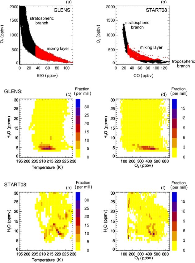
2428                                     S. Robrecht et al.: Potential of future stratospheric ozone loss in the midlatitudes

in summer, which would cause a catalytic ozone destruc-           of Morgenstern et al. (2018). In contrast, more CO2 likely
tion, has been discussed in previous studies (Anderson et al.,    causes an ozone reduction in the tropical and subtropical low-
2012, 2017; Clapp and Anderson, 2019; Schwartz et al.,            ermost stratosphere (Morgenstern et al., 2018).
2013; Robrecht et al., 2019; Schoeberl et al., 2020). Here, we       A hypothetical application of geoengineering through sul-
analyse the likelihood of the occurrence of a heterogeneous       fate injections into the stratosphere aiming to cool the tro-
chlorine activation and its impact on ozone in the lowermost      posphere would likewise affect ozone abundances in the
stratosphere in a future climate including the hypothetical ap-   lowermost stratosphere but in a different way than through
plication of sulfur injections into the stratosphere.             global warming. The troposphere-to-stratosphere-transport
   Stratospheric ozone absorbs UV radiation and thus pro-         in the midlatitudes could be reduced due to a cooling of
tects animals, plants and also human skin from radiative          the troposphere and a warming of the lower stratosphere
damage. In summer, ozone in the midlatitude lower strato-         by applying geoengineering (Visioni et al., 2017b). Further-
sphere between the tropopause and the 100 hPa level con-          more, the stratospheric H2 O abundance would increase be-
tributes ∼ 6 % (38◦ N) to 17 % (53◦ N) to the ozone col-          cause more stratospheric sulfate particles would warm the
umn (Logan, 1999). The ozone mixing ratios in the mid-            tropical tropopause layer and thus allow more H2 O to en-
latitude lower stratosphere are dominated by transport pro-       ter the stratosphere (Brewer, 1949; Dessler et al., 2013; Vi-
cesses driven by the Brewer–Dobson circulation (BDC) (e.g.        sioni et al., 2017a). An increase in stratospheric H2 O would
Ploeger et al., 2015b). However, the ozone mixing ratio in        additionally warm the stratosphere (e.g. Vogel et al., 2012;
this region is additionally affected by chemical processes.       Dessler et al., 2013). Furthermore, due to a higher H2 O
The oxidation of methane and carbon monoxide to CO2               mixing ratio, the concentration of HOx radicals increases
causes a production of ozone in the lowermost stratosphere        and thus ozone destruction in the HOx cycle accelerates
(e.g. Johnston and Kinnison, 1998; Grenfell et al., 2006),        (Heckendorn et al., 2009; Tilmes et al., 2017). Pitari et al.
while lowermost-stratospheric ozone is mainly destroyed by        (2014) describe an overall decrease in stratospheric ozone
HOx radicals (= OH, HO2 , H) (e.g. Müller, 2009). In re-          by the middle of the 21st century when geoengineering is
cent years, furthermore, the impact of heterogeneous chlo-        applied from 2020 onwards. Midlatitude ozone is mainly af-
rine activation caused by an enhancement of stratospheric         fected by an increase in heterogeneous chemistry, which in-
water vapour (in the following referred to as H2 O) through       creases ClOx (= Cl + ClO + 2 · Cl2 O2 ) and reduces NOx (=
convective overshooting has been discussed (Anderson et al.,      NO+NO2 +NO3 +2·N2 O5 ) (Pitari et al., 2014; Heckendorn
2012, 2017; Clapp and Anderson, 2019; Schwartz et al.,            et al., 2009). The increase in ClOx , which causes ozone de-
2013; Robrecht et al., 2019; Schoeberl et al., 2020).             struction in the ClOx cycle (Stolarski and Cicerone, 1974;
   Global warming will affect ozone abundances in the low-        Rowland and Molina, 1975), is balanced by the reduction
ermost stratosphere (WMO, 2018). An increase in green-            in NOx , which reduces ozone destruction in the NOx cycle
house gas (GHG) concentrations is expected to cool the            (Crutzen, 1970; Johnston, 1971), until the middle of this cen-
stratosphere (e.g. Fels et al., 1980; Iglesias-Suarez et al.,     tury (Pitari et al., 2014). In the subsequent decades, the de-
2016), slowing down gas phase ozone destruction processes.        crease in ODSs would result in a general increase in strato-
Furthermore, ozone-depleting substances (ODSs) will de-           spheric ozone (Pitari et al., 2014).
crease in the future due to the Montreal Protocol and its            In the midlatitude lowermost stratosphere in summer a fur-
amendments and adjustments (WMO, 2018). Both factors              ther chemical process may affect ozone abundances (Ander-
lead to an increase in upper-stratospheric ozone (e.g. Haigh      son et al., 2012, 2017; Clapp and Anderson, 2019; Robrecht
and Pyle, 1982; Rosenfield et al., 2002; Eyring et al., 2010;     et al., 2019). The key step of this ozone destruction mech-
Revell et al., 2012; Morgenstern et al., 2018; WMO, 2018).        anism is the chlorine activation through the heterogeneous
Since climate change would additionally lead to an accel-         reaction
eration of the BDC (e.g. Butchart and Scaife, 2001; Gar-                           het.
cia and Randel, 2008; Butchart et al., 2010; Polvani et al.,      ClONO2 + HCl −−→ Cl2 + HNO3 .                            (R1)
2018), more ozone could be transported from the tropics           Photolysis of the formed Cl2 yields active chlorine radicals,
to the poles and midlatitudes. However, an acceleration of        which can drive catalytic ozone loss cycles based on the re-
the BDC will not be uniform throughout the stratosphere           actions
(e.g. Ploeger et al., 2015a). In addition to changes in strato-
spheric transport, increasing atmospheric CH4 mixing ratios       ClO + ClO + M → ClOOCl + M,                              (R2)
can cause ozone formation in the lowermost stratosphere           ClO + BrO → Br + Cl + O2                                 (R3)
through CH4 oxidation to CO2 (Iglesias-Suarez et al., 2016).
However, comparing simulations of different models Mor-           and
genstern et al. (2018) show that an increase in CH4 can also      ClO + HO2 → HOCl + O2 .                                  (R4)
lead to an ozone reduction in the lowermost stratosphere. In-
creasing N2 O mixing ratios lead to an increase in ozone for      These cycles are already known from polar regions, namely
most model simulations, which are compared in the study           as the ClO–dimer cycle (Reaction R2; Molina and Molina,

Atmos. Chem. Phys., 21, 2427–2455, 2021                                            https://doi.org/10.5194/acp-21-2427-2021
S. Robrecht et al.: Potential of future stratospheric ozone loss in the midlatitudes                                      2429

1987) and the ClO–BrO cycle (Reaction R3; McElroy et al.,            Based on the GLENS results, box-model simulations
1986). In particular a further cycle based on Reaction (R4)       with the Chemical Lagrangian Model of the Stratosphere
first introduced by Solomon et al. (1986) for polar regions       (CLaMS) (McKenna et al., 2002b, a) are initialized, which
is expected to be relevant at activated chlorine conditions in    are used to calculate chlorine activation thresholds marking
the midlatitude lowermost stratosphere in summer (Johnson         the threshold for chlorine activation via Reaction (R1) depen-
et al., 1995; Ward and Rowley, 2016; Robrecht et al., 2019).      dent on the temperature and the H2 O mixing ratio. Hence,
For chlorine activation to occur, the temperature has to fall     the chlorine activation threshold separates conditions caus-
below a threshold temperature in polar regions (Drdla and         ing and not causing chlorine activation (and thus chlorine-
Müller, 2012), which depends on the H2 O content, the sul-        catalysed ozone loss processes known from polar regions).
fate aerosol surface area density and on altitude. Robrecht       Comparing the chlorine activation thresholds and the condi-
et al. (2019) investigated the H2 O threshold of chlorine ac-     tions in GLENS, the likelihood of chlorine activation occur-
tivation in the midlatitude lowermost stratosphere and addi-      ring is assessed and the impact of this ozone loss process on
tionally showed a minor dependence of chlorine activation         lowermost-stratospheric ozone is investigated.
on the mixing ratio of inorganic chlorine (Cly ) and nitrogen        In this paper, first the experimental setup is introduced
(NOy ).                                                           (Sect. 2). Furthermore, the temperatures and the chemical
   Since low temperatures and an enhancement of H2 O above        composition of the lowermost stratosphere today and in fu-
the background of 4–6 ppmv H2 O are crucial for chlorine          ture are analysed focusing on the GLENS results (Sect. 3).
activation and thus ozone loss to occur, Anderson et al.          The likelihood of the occurrence of chlorine activation is de-
(2012) proposed that this ozone loss mechanism is impor-          termined in Sect. 4 comparing the conditions present in the
tant for the North American lowermost stratosphere in sum-        GLENS results with calculated chlorine activation thresh-
mer. There, H2 O could penetrate into the lowermost strato-       olds. Additionally the sensitivity of the impact of this ozone
sphere through convective overshooting events within severe       loss process to temperatures is investigated assuming 2 and
storm systems (Homeyer et al., 2014; Herman et al., 2017;         5 K lower temperatures than simulated in GLENS to consider
Smith et al., 2017; Clapp and Anderson, 2019). How the in-        possible uncertainties in simulated temperatures. Finally, the
tensity and frequency of severe storm systems will change         results of this study will be discussed (Sect. 5) and summa-
over North America in the future is not clear (Anderson et al.,   rized (Sect. 6).
2017). However, an increase in stratospheric sulfate parti-
cles, e.g. caused by volcanic eruptions or the application of
geoengineering, would promote heterogeneous chlorine ac-
tivation and thus the occurrence of ozone destruction known       2     Experimental setup
from polar regions in the midlatitude lowermost stratosphere
(Anderson et al., 2012; Robrecht et al., 2019).                   The GLENS results are used as a data set representing the
   How likely and how widespread this ozone loss process          conditions in the early (2010–2020), middle (2040–2050)
could occur in the future is not yet investigated. Robrecht       and late (2090–2100) 21st century. CLaMS simulations are
et al. (2019) found that midlatitude ozone loss through en-       conducted based on the GLENS results to calculate chlorine
hanced H2 O is unlikely for today’s conditions analysing the      activation thresholds. Comparing chlorine activation thresh-
chemical process and measurements of H2 O, temperature            olds calculated from CLaMS simulations and GLENS re-
and ozone in the lowermost stratosphere. Here, we inves-          sults, we assess the likelihood of ozone loss of occurring in
tigate the likelihood of the occurrence of this ozone loss        the lowermost stratosphere above central North America in
process in the lowermost stratosphere above central North         summer today and in future scenarios.
America in summer with a focus on future climate condi-
tions. Therefore, the model results from the Geoengineering       2.1    GLENS simulations
Large Ensemble Simulations (GLENS) (Tilmes et al., 2018)
are analysed for the years 2010–2020, 2040–2050 and 2090–         The GLENS simulations were performed with version 1 of
2100. In GLENS, two future scenarios are simulated, a global      the Community Earth System Model (CESM1; Hurrell et al.,
warming scenario following the representative concentration       2013). The Whole Atmosphere Community Climate Model
pathway 8.5 (RCP8.5) scenario and the application of the          (WACCM; Marsh et al., 2013) was used as the atmospheric
sulfate geoengineering scenario, designed to keep the global      component using a 0.9◦ × 1.25◦ (latitude × longitude) grid
mean temperature to the year 2020. In general, there are dif-     and comprising 70 vertical layers up to a pressure of
ferent RCP scenarios describing different pathways of radia-      10−6 hPa. WACCM is coupled to land, sea ice and ocean
tive forcing by the year 2100. The RCP8.5 scenario assumes        models and includes fully interactive middle atmosphere
a worst-case scenario with a high GHG emission and thus a         chemistry, simplified chemistry in the troposphere as well as
large increase in the global mean temperature, which contin-      sulfate-bearing gases important for the formation of strato-
ues to increase after 2100 (Pachauri et al., 2014).               spheric sulfate (Mills et al., 2017). The three-mode version
                                                                  of the aerosol module (MAM3, Mills et al., 2016) was used

https://doi.org/10.5194/acp-21-2427-2021                                          Atmos. Chem. Phys., 21, 2427–2455, 2021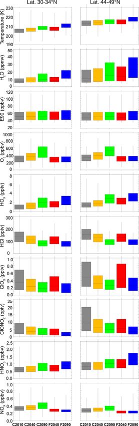
2430                                      S. Robrecht et al.: Potential of future stratospheric ozone loss in the midlatitudes

to properly represent aerosol microphysics and the sulfate         Data selection
aerosol formation from injected SO2 .
   The ability of the chosen model (CESM1 with WACCM)              GLENS provides a comprehensive global data set as-
to properly represent both atmospheric chemistry and dy-           suming two different potential scenarios and covering the
namics as well as the atmospheric response on a severe             years 2010–2100. The GLENS scenario, which follows the
stratospheric SO2 injection was shown by Mills et al. (2017).      RCP8.5 emission pathway, will lead to an increased warm-
A comparison of observations with four free-running simu-          ing of the global mean surface temperature in future. Hence,
lations for the years 1975–2016 initialized with conditions        this scenario is referred to as the “global warming scenario”
from 1 January 1975 showed a good agreement regard-                in this study. The GLENS future scenario, which assumes
ing temperature, atmospheric wind, stratospheric H2 O and          the RCP8.5 emission pathway together with stratospheric
ozone. In particular, the model depicts the quasi-biennial os-     SO2 injections to keep the global mean surface temperature
cillation (QBO) and the “tape recorder” (Mills et al., 2017).      from warming, is here referred to as the “geoengineering sce-
Simulations of the Mt. Pinatubo eruption of 1991 were in           nario”. Only specific decades and a specific region – namely
agreement with the observed aerosol optical depth. Espe-           air masses in the lowermost stratosphere above central North
cially, the radiative impacts (namely the absorbed solar radi-     America in the early, middle and late 21st century – are con-
ation and the outgoing long-wave radiation) agreed very well       sidered using the 10-day instantaneous GLENS output for
with the observations, which is important to properly simu-        the months June, July and August.
late the effect of stratospheric SO2 injections on stratospheric      In total five cases are analysed which are determined
chemistry and dynamics.                                            through the GLENS scenario and the decade. The case
   An extensive overview of the GLENS simulations is given         C2010 describes conditions in the early 21st century (2010–
elsewhere (Tilmes et al., 2018). Briefly, GLENS simulations        2020) based on the GLENS global warming scenario. The
were performed to provide a comprehensive data set for             conditions for the middle (2040–2050) and the end (2090–
studying the limitations, side effects and risks of geoengi-       2100) of the 21st century following the global warming sce-
neering. The GLENS study comprises three ensemble mem-             nario are referred to as cases C2040 and C2090, respectively.
bers from the year 2010 to the end of the 21st century follow-     The cases of the geoengineering scenario are named F2040
ing the RCP8.5 scenario. Since only the first of these simu-       and F2090 for the middle and the end of the 21st century,
lations was run until 2099, we choose the first of these en-       respectively (“F” stands for the “Feedback” mechanism of
semble members for our study. We furthermore choose the            the SO2 injections). An overview of the considered cases is
first of 20 ensemble members of the geoengineering scenario        given in Table 1 together with the global mean temperature
comprising the years 2020–2099.                                    increase reached in that case compared to the conditions of
   The geoengineering scenario of GLENS is based on the            the years 2010–2020 and the injected amount of SO2 .
RCP8.5 scenario but aims to hold the global mean tem-                 GLENS results are selected for a latitude range of 30.6–
perature, the inter-hemispheric temperature gradient and the       49.5◦ N and a longitude range of 72.25–124.75◦ W (grey area
Equator-to-pole gradient at the Earth surface at the level of      in Fig. 1a) because for this area the reliability of the GLENS
the year 2020 by applying stratospheric sulfur injections (for     C2010 results could be analysed in comparison with air-
more details; see Kravitz et al., 2017). To reach the temper-      craft measurements of the SEAC4 RS (Studies of Emissions
ature targets, SO2 is simultaneously injected beginning from       and Atmospheric Composition, Clouds and Climate Cou-
the year 2020 at four injection locations. These are chosen        pling by Regional Surveys) and START08 (Stratosphere–
to be at 15◦ N and 15◦ S at an altitude of 25 km and at 30◦ N      Troposphere Analyses of Regional Transport 2008) cam-
and 30◦ S at an altitude of 22.8 km based on previous studies      paigns. Since the ozone loss process focused on in this study
about the injection location on the effectiveness of geoengi-      is expected to occur most likely in summer, only the months
neering (MacMartin et al., 2017; Tilmes et al., 2017). The         June, July and August are considered. As shown in Fig. 1b
amount of injected sulfur at each location is determined us-       the tropopause altitude varies depending on latitude and the
ing a feedback algorithm that annually adjusts the location        considered case. Since the tropopause altitude varies signifi-
rates (MacMartin et al., 2014; Kravitz et al., 2016, 2017). To     cantly above central North America, the latitude range is di-
reach the temperature targets, in the GLENS geoengineering         vided into four bins (30–35, 35–40, 40–44 and 44–49◦ N),
scenario more than 50 Tg SO2 would have been emitted at the        but in this study the focus is on subtropical latitude band (30–
end of the 21st century. This is 5 times the emitted amount of     35◦ N) with a more likely subtropical character of the chem-
sulfur by the Mt. Pinatubo eruption in the year 1992 (Tilmes       ical composition and the extratropical latitude band (44–
et al., 2018). However, other models than the WACCM do             49◦ N) representing the chemical composition of the extra-
need to inject other amounts of SO2 into the stratosphere to       tropics around the tropopause.
keep the global mean surface temperature constant (Timm-              This study focuses on the mixing layer between tropo-
reck et al., 2018). Hence, it should be noted that generally       spheric and stratospheric air located in the lowermost strato-
there is a certain range of uncertainty in the SO2 amount          sphere above central North America (blue illustrated in
needed.                                                            Fig. 1a). Without mixing between tropospheric and strato-

Atmos. Chem. Phys., 21, 2427–2455, 2021                                              https://doi.org/10.5194/acp-21-2427-2021
S. Robrecht et al.: Potential of future stratospheric ozone loss in the midlatitudes 2431
Table 1. Overview of the cases analysed in this study. In addition to the years considered, the underlying emission scenario in the GLENS
simulation, the global temperature increase (referred to 2010–2020) and the SO2 amount injected by that time period are given for each case.
Case Years GLENS scenario emission scenario global temperature SO2
increase (K) injected (Tg)
C2010 2010–2020 global warming RCP8.5 0.0 0.0
C2040 2040–2050 global warming RCP8.5 1.8 0.0
C2090 2090–2100 global warming RCP8.5 6.0 0.0
F2040 2040–2050 geoengineering RCP8.5 −0.1 14.4
F2090 2090–2100 geoengineering RCP8.5 0.1 49.0
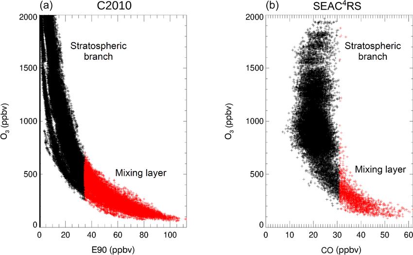
spheric air, correlations of trace gases mainly released in the on GLENS results. Therefore, considered GLENS results are
troposphere (e.g. CO) and mainly produced in the strato- divided into different latitude regions, pressure levels and
sphere (e.g. O3 ) form an “L shape” (Pan et al., 2004; Vo- ozone mixing ratios as shown in Table 2. Any combina-
gel et al., 2011) consisting of a tropospheric and a strato- tion of latitude, pressure and ozone range is referred to as
spheric branch. A mixing layer between tropospheric and a data group. The pressure levels are chosen based on the
stratospheric air masses additionally generates mixing lines vertical levels used in GLENS. The GLENS results are sepa-
in the tracer–tracer space resulting in “cutting off” the corner rated into different ozone ranges because higher ozone mix-
of the L shape (e.g. Hoor et al., 2002; Pan et al., 2004; Vogel ing ratios are correlated with higher Cly mixing ratios, which
et al., 2011). The mixing layer in midlatitudes is located close promote the likelihood of heterogeneous chlorine activation
the thermal tropopause, with a significant part in the lower- occurring and its impact on ozone (Robrecht et al., 2019).
most stratosphere. Air masses within the mixing layer are Furthermore, based on the ozone mixing ratio considered air
characterized by relatively high H2 O from the troposphere masses can be divided into those with a chemical composi-
compared to typically low stratospheric H2 O amounts and tion of air masses typical of the troposphere (low ozone) and
by O3 and Cly higher than usually found in the upper tropo- those with a chemical composition more typical of the strato-
sphere from mixing with stratospheric air. Furthermore, the sphere (high ozone).
temperatures are low due to the location close to the ther- Stratospheric chemistry is simulated along artificial 10-
mal troposphere. Hence, the lowermost-stratospheric mixing day trajectories, which are designed to calculate the chlorine
layer shows conditions for which heterogeneous chlorine ac- activation threshold for each data group. Therefore, the tra-
tivation most likely occurs and is therefore the focus of this jectories are located at a specific point in the stratosphere de-
study. termined as 102.5◦ W (middle longitude over the considered
Since the tropopause altitude and thus the altitude range longitude range) and the middle pressure and latitude of the
of the mixing layer varies for different latitudes and future specific data group (e.g. 32.5◦ N for the latitude range 30–
scenarios, the selected altitude range for air masses in the 35◦ N and 80 hPa for the pressure range of 70–90 hPa). As
lowermost-stratospheric mixing layer is determined so that chemical initialization for the CLaMS box model, the me-
it may vary in the considered cases. The lower boundary of dian mixing ratio is taken of each trace gas from GLENS in a
the data selected is chosen to be the thermal tropopause cal- data group. For each of the five cases (see Table 1) and each
culated according to the WMO definition within GLENS for data group (Table 2), chemical simulations are conducted as-
each time step by the model. The upper boundary is deter- suming constant H2 O varying from 4–30 ppmv in steps of
mined by a mixing ratio of 35 ppbv of the artificial E90 tracer. 1 ppmv and a constant temperature varying from 195–230 K
This is a passive tropospheric tracer in WACCM globally re- in 1 K steps resulting in a total of 455 000 box-model simu-
leased with a lifetime of 90 days, a mixing ratio of ∼ 90 ppbv lations. Hereafter, instead of pressure ranges a pressure level
at the tropopause and a strong decrease in the lowermost as given in Table 2 is used in the text.
stratosphere (Abalos et al., 2017). Since the E90 tracer is Heterogeneous chemistry is only considered here to take
emitted continuously throughout the GLENS simulations, it place on liquid particles to ensure a comparability to the
is independent of possible changes in the emission rates of study of Anderson et al. (2012). Further, only a very low frac-
other tropospheric trace gases and therefore a good marker tion of GLENS data points shows conditions cold enough for
of the fraction of tropospheric air in the considered air mass. the formation of ice particles. As initialization for liquid par-
ticles, the particle number density and the gas phase equiv-
2.2 CLaMS simulations alent of H2 SO4 is needed, taken from monthly GLENS data
as the median of a data group.
Box-model simulations with CLaMS (e.g. McKenna et al.,
2002b, a) are performed to determine chlorine activation
thresholds. CLaMS simulations are further initialized based
https://doi.org/10.5194/acp-21-2427-2021 Atmos. Chem. Phys., 21, 2427–2455, 2021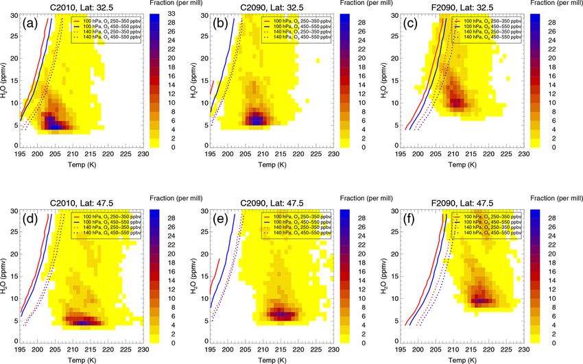
2432 S. Robrecht et al.: Potential of future stratospheric ozone loss in the midlatitudes
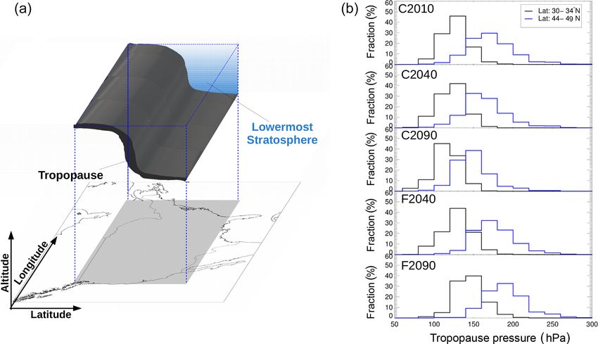
Figure 1. Schematic overview of the selected data region over North America (a). The position of the tropopause over central North Amer-
ica in summer is illustrated in black, and the mixing layer is directly located above the tropopause in the lowermost stratosphere (blue).
Panel (b) presents the tropopause pressure released from GLENS in this region depending on the latitude range and all considered cases (see
Table 1.)
Table 2. Overview of the latitude, pressure, ozone, H2 O and temperature ranges, for which CLaMS simulations are conducted. Each com-
bination of latitude, pressure and ozone range is summarized in a data group resulting in 100 different data groups. For a better overview in
this paper, pressure levels are used to describe the pressure ranges (e.g. 80 hPa level for the pressure range 70–90 hPa).
Latitude (◦ N) 30–35 35–40 40–44 44–49
Pressure range (hPa) 70–90 90–110 110–130 130–150 150–300
Pressure level 80 hPa 100 hPa 120 hPa 140 hPa 160 hPa
O3 (ppbv) 150–250 250–350 350–450 450–550 550–650
H2 O (ppmv) 4–30 in steps of 1 ppmv
Temperature (K) 195–230 in steps of 1 K
Calculation of the chlorine activation thresholds tion threshold for the considered latitude, pressure and ozone
range.
The chlorine activation threshold for each data group defines
the conditions that allow chlorine-catalysed ozone destruc-
tion. Hence, the fraction of GLENS air masses showing these 3 Analysing lowermost-stratospheric GLENS results
conditions corresponds to the likelihood that ozone destruc- above central North America
tion occurs as a result of heterogeneous chlorine activation in
the North American lowermost stratosphere. The selected GLENS results are used as a data set represent-
Chlorine activation thresholds are calculated for each data ing the conditions and chemical composition in the mixing
group. Therefore, the H2 O and temperature conditions caus- layer in the North American lowermost stratosphere in sum-
ing chlorine activation within a simulation are identified. mer for all considered cases for future and today’s conditions.
Chlorine activation is assumed to have occurred if ClOx con-
tributes 10 % of Cly within the first 5 days of a CLaMS 3.1 Comparing the GLENS mixing layer today with
simulation. For each H2 O value, the maximum temperature measurements
at which chlorine activation occurs is determined to be the
temperature threshold for heterogeneous chlorine activation. The reliability of the selected GLENS mixing layer of the
The array of this temperature threshold depends on a spe- C2010 case is analysed by comparing the mixing layer in
cific H2 O mixing ratio, which defines the chlorine activa- case C2010 for the latitude range 30–35◦ N with the mix-
Atmos. Chem. Phys., 21, 2427–2455, 2021 https://doi.org/10.5194/acp-21-2427-2021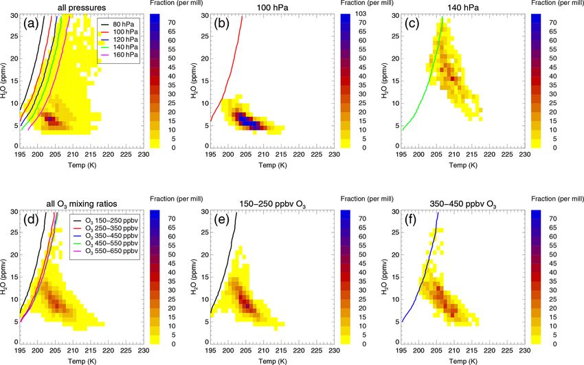
S. Robrecht et al.: Potential of future stratospheric ozone loss in the midlatitudes                                          2433

                                                                      spheric air by holding more than 35 ppbv of the E90 tracer.
                                                                      In the mixing layer deduced from SEAC4 RS measurements,
                                                                      considered air masses lay above the tropopause as well and
                                                                      are separated here from the stratospheric branch by holding
                                                                      a CO mixing ratio of more then 31 ppbv.
                                                                         Figure 3a and b show the relative distribution of oc-
                                                                      currence frequency of data points in the mixing layer of
                                                                      case C2010 in the temperature–H2 O (a, c) and ozone–H2 O
                                                                      (b, d) correlation hereafter referred to as relative frequency
                                                                      distribution. For the relative frequency distribution in the
                                                                      temperature–H2 O correlation, the number of data points in
                                                                      the mixing layer of case C2010 in all temperature and H2 O
                                                                      bins of the size of 1 K × 1 ppmv H2 O (Fig. 3a, c) are cal-
Figure 2. Tracer–tracer correlations for the results of case C2010    culated considering the whole H2 O and temperature range
in a latitude range from 30–35◦ N (a) and SEAC4 RS measure-           given in Table 2. For the relative frequency distribution
ments (b) consist of a stratospheric branch (black) and of the mix-   in the ozone–H2 O correlation (Fig. 3b, d), the number of
ing layer between stratospheric and tropospheric air masses (red).    data points in all ozone and H2 O bins of the size 10 ppbv
The mixing layer is determined to be located above the tropopause     O3 × 1 ppmv H2 O are calculated. The number of data points
and showing more than 35 ppbv E90 in case C2010 and more than         of each temperature–H2 O (O3 –H2 O) bin is normalized by
31 ppbv CO in SEAC4 RS measurements.
                                                                      the total number of data points found in the mixing layer of
                                                                      case C2010. These fractions are colour-coded in Fig. 3. The
                                                                      relative frequency distribution of data points in the mixing
ing layer derived from SEAC4 RS ER2 aircraft measurements             layer derived from SEAC4 RS measurements in the same way
in August and September 2013. The SEAC4 RS campaign                   is shown in Fig. 3c and d.
was based in Houston (Texas) and one aim was to investi-                 Comparing the SEAC4 RS mixing layer with that of case
gate the impact of deep convective clouds on the H2 O con-            C2010 yields a similar relative frequency distribution regard-
tent in the lowermost stratosphere (Toon et al., 2016). Hence,        ing temperature and H2 O conditions. Above 5 ppmv H2 O,
SEAC4 RS measurements represent moist and cold condi-                 the maximum fraction of C2010 and SEAC4 RS data resides
tions enhancing the likelihood of heterogeneous chlorine ac-          in the same H2 O and temperature range of 201–207 K and
tivation occurring. Here, SEAC4 RS trace gas measurements             5–8 ppmv H2 O (Fig. 3a, c). However, SEAC4 RS data show
are used for CO (Harvard University Picarro cavity ring-              a higher fraction at lower temperatures of 197–200 K and a
down spectrometer (HUPCRS); Werner et al., 2017), O3 (Na-             higher fraction of data in case C2010 has lower H2 O mixing
tional Oceanic and Atmospheric Administration (NOAA)                  ratios than 5 ppmv. Furthermore, C2010 data spread over a
unmannsed aircraft system O3 instrument; Gao et al., 2012)            broader H2 O range.
and H2 O (Harvard Lyman-α photo fragment fluorescence hy-                The SEAC4 RS mixing layer and the mixing layer in case
grometer (HWV); Weinstock et al., 2009). Since GLENS                  C2010 show a similar distribution regarding the H2 O–O3
is performed with a global model, the GLENS data cover                correlation (Fig. 3b, d). A significant fraction of all data
a broader range in space (regarding altitude and area) than           corresponds to an ozone range of 200–350 ppbv, but in the
SEAC4 RS aircraft measurements, which were locally taken              C2010 data a higher fraction holds low H2 O mixing ratios
up to an altitude of 20 km. Hence, GLENS and SEAC4 RS air             with an ozone mixing ratio of 400–450 ppbv.
masses have a different spatial distribution in the lowermost            In addition to SEAC4 RS measurements, data in the
stratosphere above North America.                                     GLENS mixing layer of case C2010 are compared with
   The mixing layer between stratospheric and tropospheric            measurements sampled during the Stratosphere–Troposphere
air masses in the SEAC4 RS measurements is assumed to con-            Analyses of Regional Transport (START08) campaign (Pan
sist of measurements above the tropopause with a CO mixing            et al., 2010), which covers a larger latitude range over cen-
ratio of more than 31 ppbv. This CO boundary is selected to           tral North America than the SEAC4 RS measurements. The
allow an O3 range similar to that of the GLENS mixing layer           START08 campaign was designed to characterize the trans-
(up to ∼ 750 ppbv) and agrees with observations in the study          port pathways in the extratropical tropopause region using
by Pan et al. (2004), where mixed air masses between tropo-           the U.S. National Science Foundation (NSF) Gulfstream V
sphere and stratosphere were described to hold usually more           (GV) research aircraft. START08 measurements show a good
than ∼ 30 ppbv CO. In Fig. 2, the mixing layer of case C2010          overall agreement with GLENS results in case C2010, in
(a) and the SEAC4 RS mixing layer (b) are marked in red,              spite of the fact that a higher fraction of air masses sampled
while the stratospheric branch is shown in black. Air in the          during START08 has temperatures higher than 215 K caused
GLENS mixing layer is separated from tropospheric air by              by the maximum flight height of the GV of ∼14.5 km (for
being located above the thermal tropopause and from strato-           more information see Appendix A).

https://doi.org/10.5194/acp-21-2427-2021                                              Atmos. Chem. Phys., 21, 2427–2455, 2021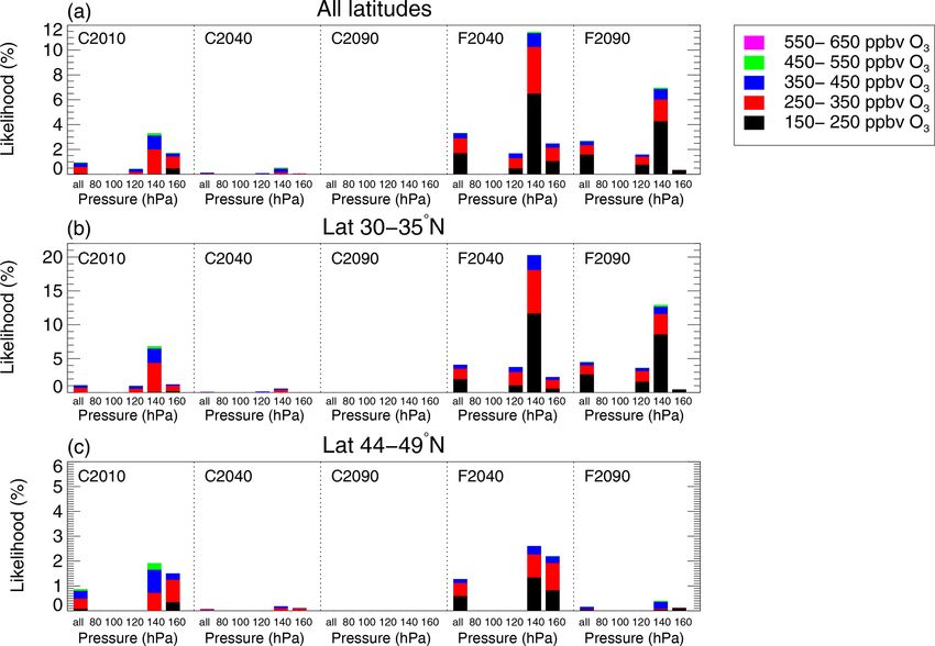
2434 S. Robrecht et al.: Potential of future stratospheric ozone loss in the midlatitudes
Figure 3. Comparison of the relative distribution of the occurrence frequency of data points in the GLENS mixing layer of case C2010
between stratospheric and tropospheric air masses (a, b) with measurements of the SEAC4 RS aircraft campaign (c, d). Panels (a) and
(c) show the relative frequency distribution regarding H2 O and temperature conditions and panels (b) and (d) regarding H2 O and ozone
mixing ratios. The relative frequency distribution is derived by calculating the number of data points found in a specific temperature and
H2 O bin (1 K × 1 ppmv H2 O; a, c) or ozone and H2 O bin (10 ppbv O3 × 1 ppmv H2 O; b, d) considering all H2 O and temperature (ozone)
ranges given in Table 2. The number of data points of each temperature–H2 O (O3 –H2 O) bin is normalized by the total number of data points.
The colour scheme marks these fractions.
In general, data points from the modelled case C2010 rep- Fig. 4, agrees well with the F2040 case (red) and the F2090
resenting the mixing layer have a good overall agreement case (blue). For cases with global warming, the ozone mix-
with data points in the mixing layer deduced from aircraft ing ratio is significantly higher in case C2040 (yellow) and
measurements above North America. Measurements during C2090 (green) especially for low E90 concentrations. The
SEAC4 RS sampled convective injections of H2 O into the enhancement of ozone in the mixing layer could be caused
stratosphere (Toon et al., 2016; Smith et al., 2017; Herman by changes in atmospheric transport or chemistry. Global
et al., 2017) and thus provide unusually cold and moist con- warming is expected to increase upper-stratospheric ozone
ditions for the lowermost stratosphere, which are lower than and accelerate the BDC. In the considered latitude range, this
the temperatures in the simulated C2010 case (∼ 195–209 K leads to more ozone transported downwards into the lower-
mainly prevailing in SEAC4 RS instead of ∼ 201–209 K in most stratosphere from high altitudes (Iglesias-Suarez et al.,
case C2010). To consider the impact of this temperature bias 2016).
on ozone further simulations are preformed (see Sect. 4.5) Besides changes in transport, ozone in the midlatitude
assuming temperatures to be 2 and 5 K lower than found in mixing layer could be affected by changes in chemistry
GLENS. (e.g. through chlorine activation). The conditions causing
heterogeneous chlorine activation are determined first of all
3.2 Change in the chemical composition of the mixing by temperature and H2 O mixing ratios. Furthermore, Cly and
layer NOy mixing ratios affect the threshold between conditions,
which may or may not lead to chlorine activation. The dis-
The chemical composition of the mixing layer changes in tribution of temperatures and several trace gas mixing ratios
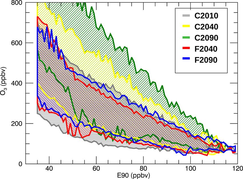
the GLENS future scenarios. In Fig. 4, the E90–O3 cor- within the GLENS mixing layer for all cases considered is
relation is shown for all considered cases (see Table 1). shown in Fig. 5 for the subtropical (30–35◦ N) and the extrat-
In the global warming future scenario (C2040, C2090), the ropical (44–49◦ N) latitude band over central North America.
O3 mixing ratio increases during the 21st century, but the In all future scenarios, temperatures and H2 O mixing ra-
ozone mixing ratio in the geoengineering scenario (F2040, tios increase (Fig. 5). In the subtropical latitude band, the
F2090) remains in a similar range of ∼ 200–600 ppbv as median temperature increases by ∼ 3 K from today (case
in case C2010. The correlation between ozone and the ar- C2010) to the end of the 21st century assuming a global
tificial tropospheric tracer E90 for C2010 (grey), shown in warming scenario (C2090) and by ∼ 5.5 K when applying
Atmos. Chem. Phys., 21, 2427–2455, 2021 https://doi.org/10.5194/acp-21-2427-2021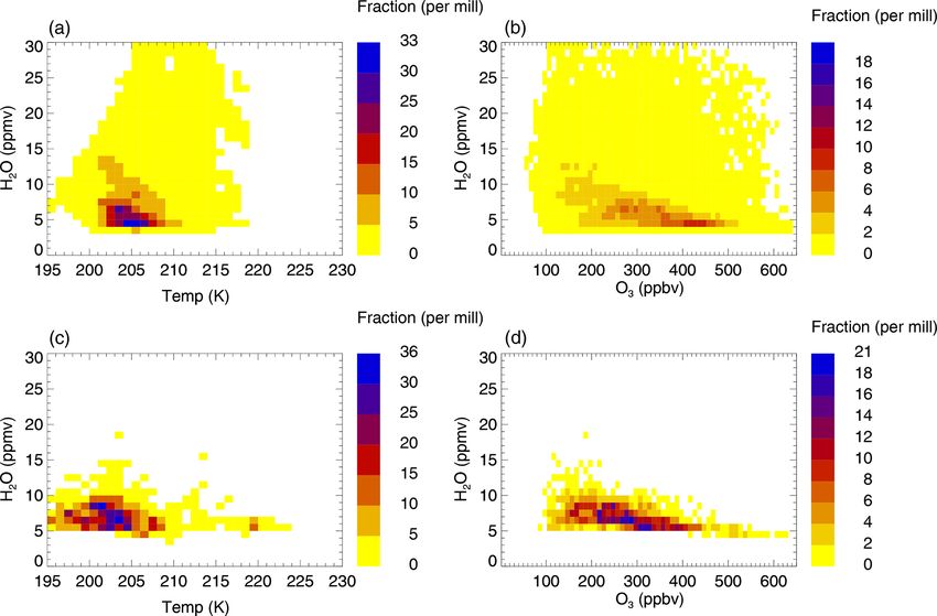
S. Robrecht et al.: Potential of future stratospheric ozone loss in the midlatitudes                                                 2435

Figure 4. O3 –E90 correlation in the GLENS mixing layer for today
(C2010) and the future scenarios considering both global warming
(C2040, C2090) and additional geoengineering (F2040, F2090). An
overview of the presented cases is given in Table 1.

geoengineering (case F2090). In the extratropical latitude
band, the temperature is higher and shows a similar increas-
ing trend. H2 O mixing ratios are higher in the extratropi-
cal latitude band than in the subtropical band and spread
over a broader range. In both latitude ranges and future sce-
narios the H2 O content increases until the end of the 21st
century driven by increasing temperatures of the tropical
tropopause layer. An increase in H2 O enhances HOx mix-
ing ratios (Fig. 5) and thus accelerates ozone destruction in
the HOx cycle.
   The HCl and ClOx mixing ratios decrease in the GLENS
simulations for both future scenarios due to the implemen-
tation of boundary conditions in WACCM according to the
Montreal Protocol and its amendments and adjustments.
However, the median ClOx mixing ratio is higher by ∼ 8
(30–34◦ N)–22 % (44–49◦ N) in the F2040 case than in the
C2040 case. This could be due to a reduced NOx mixing ratio
in the F2040 case. In both future scenarios, the HNO3 mixing
ratio increases until the year 2100 (Fig. 5). For global warm-
ing, the NOx mixing ratio increases as well. It decreases
in the geoengineering scenario because HNO3 formation is
accelerated through heterogeneous reactions favoured by a
higher aerosol abundance and increasing temperatures en-
hancing the NO2 /NO ratio. Less NOx causes less ClOx to             Figure 5. Distribution of temperatures and several trace gas mixing
be bound in ClONO2 , thus resulting in more gas phase ClOx          ratios in the GLENS mixing layer for case C2010 and future sce-
in the geoengineering scenario. Additionally, the occurrence        narios considering both global warming (C2040, C2090) and sul-
of heterogeneous chlorine activation could yield an enhance-        fate geoengineering (F2040, F2090) (see Table 1). The frequency
ment of ClOx in the geoengineering scenario due to an en-           distribution is illustrated as box plots, where the upper and lower
hanced aerosol abundance.                                           quartile (75 % and 25 %) of the data set is marked by the upper and
                                                                    lower end of the box. The median of the temperature or mixing ratio
   The changes in chemistry may affect the future ozone
                                                                    values within the mixing layer is illustrated by the horizontal line in
abundance in the lowermost stratosphere. The median ozone
                                                                    the box. Ends of vertical lines mark the minimum and the maximum
mixing ratio increases by 60 %–67 % until the year 2100 in          value of the considered data.
the global warming scenario but remains at today’s level in

https://doi.org/10.5194/acp-21-2427-2021                                               Atmos. Chem. Phys., 21, 2427–2455, 2021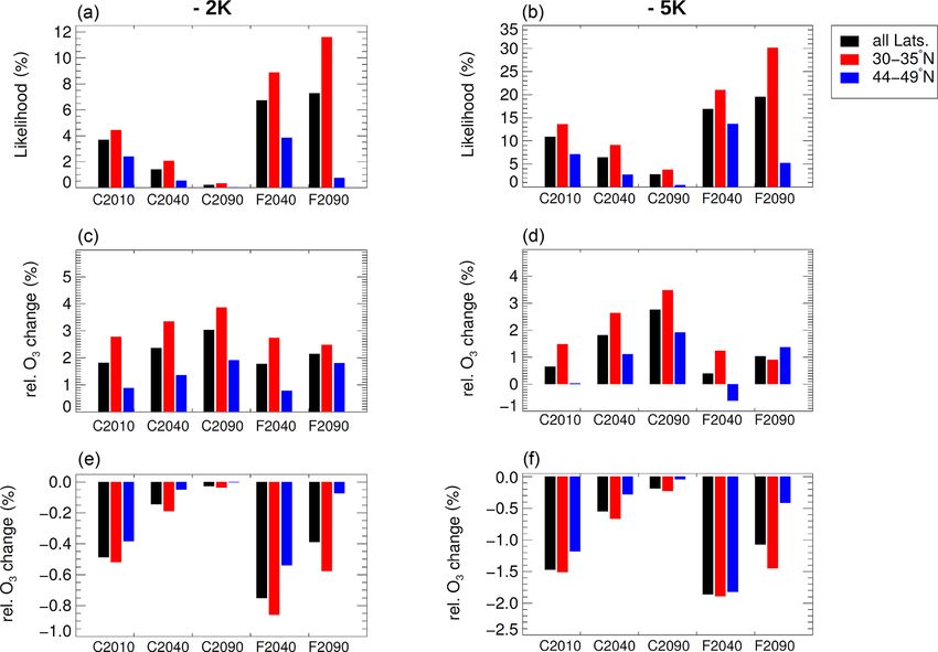
2436                                      S. Robrecht et al.: Potential of future stratospheric ozone loss in the midlatitudes

the geoengineering scenario (Fig. 5). The partitioning be-         for all pressure levels in the considered latitude and ozone
tween active radicals (ClOx , NOx ) and reservoir species          range (30–35◦ N, 350–450 ppbv O3 ).
(HCl, HNO3 ) differs between the global warming (C2040,               At higher pressure levels (lower altitudes), the chlorine ac-
C2090) and the geoengineering (F2040, F2090) cases re-             tivation threshold is shifted allowing chlorine activation to
sulting in a different chemical impact on ozone. The likeli-       occur at higher temperatures (Fig. 6a). This shift is due to an
hood of the occurrence of ozone loss caused by heteroge-           increasing liquid particle formation as well as more ClONO2
neous chlorine activation may differ as well in the future         absorbed by an aerosol particle at higher pressures. The het-
scenarios because the heterogeneous chlorine activation is         erogeneous chlorine activation rate of Reaction (R1) is deter-
stronger for low temperatures and enhanced H2 O mixing val-        mined by the ClONO2 uptake into the aerosol particle (Shi
ues. The likelihood of heterogeneous chlorine activation oc-       et al., 2001). Air masses lying on the left side of the chlo-
curring and its impact on the ozone chemistry are analysed         rine activation threshold show chlorine activation. The rela-
below in the subsequent section.                                   tive frequency distribution shown in Fig. 6 a is related to all
                                                                   air masses with 350–450 ppbv ozone in a latitude range of
                                                                   30–35◦ N. Some data points cross various activation thresh-
4     Comparison of GLENS results with chlorine                    olds. However, only data points crossing the chlorine activa-
      activation thresholds                                        tion threshold and in addition corresponding to the pressure
                                                                   level of the activation threshold will yield activated chlorine.
The H2 O and temperature range in which heterogeneous              As an example, the chlorine activation thresholds at the 100
chlorine activation occurs, is determined by calculating chlo-     and 140 hPa level are plotted together with the GLENS rel-
rine activation thresholds for the specific chemical compo-        ative frequency distribution corresponding to the same data
sition using the CLaMS model. For each case (Table 1), the         group (Fig. 6b, c). Air masses in the 100 hPa level (Fig. 6b)
fraction of all air masses in the GLENS mixing layer between       are colder and dryer than those at 140 hPa (Fig. 6c). Hence,
the troposphere and the stratosphere with conditions leading       at the 100 hPa level no chlorine will be activated (there are
to chlorine activation accounts for the likelihood that chlorine   no data corresponding to an H2 O–temperature bin on the left
activation occurs. The chlorine activation threshold is deter-     side of the threshold line) and chlorine activation occurs for
mined based on the composition of GLENS air masses in              the 140 hPa level only for data points with a high H2 O mixing
the mixing layer between tropospheric and stratospheric air        ratio.
(see Sect. 3). Chlorine activation thresholds are calculated for      In Fig. 6d–f, the H2 O—temperature relative frequency dis-
all cases (see Table 1) with CLaMS (see Sect. 2.2) for four        tribution and the chlorine activation thresholds are presented
latitude ranges from 30–49◦ N, five pressure ranges between        for a pressure level of 120 hPa. The impact of the ozone mix-
70 and 300 hPa and five different ozone ranges from 150–           ing ratios on the chlorine activation threshold is illustrated.
650 ppbv (see Table 2). Ozone values lower than 150 ppbv           Figure 6d shows the GLENS H2 O–temperature relative fre-
are not considered here because only a minor fraction of           quency distribution and the chlorine activation thresholds for
air parcels shows less than 150 ppbv ozone. Furthermore, a         all data groups corresponding to the selected latitude range
critical ozone amount has to be exceeded for chlorine ac-          and pressure level (30–35◦ N, 120 hPa). Higher ozone mix-
tivation to occur (von Hobe et al., 2011) because a higher         ing ratios are related to higher Cly amounts. Hence, an in-
ozone mixing ratio causes a higher ClO/Cl ratio and thus           crease in ozone shifts the chlorine activation threshold to
more ClONO2 is formed. This is important for heteroge-             higher temperatures (Fig. 6d). However, considering the rel-
neous chlorine activation in Reaction (R1) to occur.               ative frequency distribution of specific data groups with dif-
                                                                   ferent ozone levels, data points with more ozone are warmer
4.1    Analysis of chlorine activation thresholds                  than those with less ozone (Fig. 6e, f).
                                                                      In the future scenarios, the H2 O–temperature relative fre-
Both the chlorine activation threshold and the H2 O–               quency distribution as well as the chlorine activation thresh-
temperature relative frequency distribution vary depending         olds vary. In Fig. 7 the H2 O–temperature relative frequency
on the assumed pressure and ozone level and thus for differ-       distribution is shown for the cases C2010, C2090 and F2090.
ent data groups. An example for the impact of the pressure         The relative frequency distributions are shown for the sub-
and ozone range on the H2 O–temperature relative frequency         tropical latitude band (30–35◦ N, Fig. 7a–c) and for the ex-
distribution and the chlorine activation threshold is shown in     tratropical latitude band (44–49◦ N, Fig. 7d–f). For each case
Fig. 6 for the mixing layer of case C2010 in the latitude range    shown, additionally, a selection of chlorine activation thresh-
of 30–35◦ N.                                                       olds is shown. These are related to different ozone and pres-
   The H2 O–temperature relative frequency distribution is         sure levels and give a range of uncertainty for the H2 O and
shown (Fig. 6a–c) for an ozone range of 350–450 ppbv. The          temperature ranges causing chlorine activation.
H2 O- and temperature-dependent chlorine activation thresh-           In agreement with the changes in the conditions in the mix-
olds are marked as a line for different pressure levels (see       ing layer described in Sect. 3, the future H2 O–temperature
Table 2). In Fig. 6a, chlorine activation thresholds are plotted   relative frequency distributions (C2090 in Fig. 7b, F2090 in

Atmos. Chem. Phys., 21, 2427–2455, 2021                                              https://doi.org/10.5194/acp-21-2427-2021
S. Robrecht et al.: Potential of future stratospheric ozone loss in the midlatitudes 2437 Figure 6. H2 O–temperature relative frequency distributions and chlorine activation thresholds of different data groups (see Table 2) for the C2010 case and a latitude range of 30–35◦ N. The H2 O–temperature relative frequency distribution is illustrated as a colour scheme. The colour marks the fraction of the considered data corresponding to an H2 O and temperature bin (1 ppmv H2 O × 1 K). The H2 O- and temperature-dependent chlorine activation thresholds are marked as a line. Panels (a)–(c) are related to data groups with an ozone mixing ratio of 350–450 ppbv: all data in the considered latitude and ozone range (30–35◦ N, 350–450 ppbv O3 ) (a); the data group defined by a latitude of 30–35◦ N, an ozone mixing ratio of 350–450 ppbv O3 and the 100 hPa pressure level (b); and the data group defined by a pressure level of 140 hPa and the same latitude and ozone range (c). Panels (d)–(f) are related to data groups with a pressure level of 120 hPa: all data in the considered latitude and pressure level (30–35◦ N, 120 hPa) (d); the data group defined by a latitude of 30–35◦ N, a pressure level of 120 hPa and an ozone mixing ratio of 150–250 ppbv O3 (e); and the data group defined by an ozone mixing ratio of 350–450 ppbv and the same latitude and pressure level (f). Fig. 7c) are both moister and warmer than the conditions In each case, the H2 O and temperature bins marked by the today (C2010, Fig. 7a). However, the geoengineering case chlorine activation thresholds to potentially cause heteroge- F2090 exhibits data significantly warmer and moister than neous chlorine activation are in good agreement for both lat- reached in the global warming case C2090. In the extrat- itude ranges presented. Since the temperatures of the mixing ropical latitude band (Fig. 7d–f), temperatures are generally layer are higher in the extratropical latitude band, the fraction higher than in the subtropical latitude range. of air masses crossing the chlorine activation threshold and Considering the chlorine activation thresholds in Fig. 7, thus causing chlorine activation is lower in that latitude range the largest fraction of air masses corresponds to temperatures (44–49◦ N) than in the subtropical latitude band (30–35◦ N). greater than the chlorine activation thresholds. The chlorine There are some chlorine activation thresholds that cannot activation thresholds for the C2090 case are shifted to lower be reported when the H2 O mixing ratio exceeds a certain temperatures compared to case C2010 because of the lower value (e.g. Fig. 7e, 100 hPa, 250–350 ppbv O3 ). At such high chlorine abundance (a higher Cly mixing ratio promotes het- H2 O mixing ratios, HCl is absorbed strongly into the aerosol erogeneous chlorine activation; Robrecht et al., 2019). In particles, reducing gas phase Cly , and thus less ClONO2 contrast, in the geoengineering scenario F2090 chlorine ac- may be formed. Since chlorine is activated in Reaction (R1) tivation can occur at higher temperatures than today in spite (HCl + ClONO2 ), less ClONO2 leads to a lower chlorine ac- of the lower chlorine amount. This is caused by the higher tivation rate. HCl uptake into supercooled water particles aerosol loading due to the applied geoengineering. was also found to occur after volcanic eruptions resulting https://doi.org/10.5194/acp-21-2427-2021 Atmos. Chem. Phys., 21, 2427–2455, 2021
2438                                        S. Robrecht et al.: Potential of future stratospheric ozone loss in the midlatitudes

Figure 7. H2 O–temperature relative frequency distributions and examples for chlorine activation thresholds for the cases C2010 (a, d) and
the future scenarios at the end of the 21st century assuming global warming (C2090, b, e) and additional geoengineering (F2090, c, f) for the
subtropical latitude band (30–35◦ N, a–c) and the extratropical band (44–49◦ N, d–f). The colour marks the fraction of the considered data
corresponding to an H2 O and temperature bin (1 ppmv H2 O × 1 K). The H2 O- and temperature-dependent chlorine activation threshold is
marked as a line for exemplarily chosen data groups specified in the legend of each panel.

in an “HCl scavenging”, which may protect the ozone layer                vation results in only few air masses with conditions suitable
(Tabazadeh and Turco, 1993). In our study the effect of HCl              to activate chlorine. Thus, chlorine activation thresholds have
uptake is negligible if the Cly mixing ratio is high enough.             to be compared with air masses in GLENS corresponding to
But if the Cly mixing ratio is low (e.g. in a low ozone range            the same data group regarding pressure, ozone and latitude
in the years 2090–2099), reducing gas phase Cly by absorb-               range as the calculated chlorine activation threshold to de-
ing HCl into the aerosol results in no activation of chlorine.           duce the likelihood that chlorine activation occurs.
Hence, there is no chlorine activation for these conditions.
   Summarizing, the H2 O- and temperature-dependent chlo-                4.2   Likelihood of ozone destruction today and in the
rine activation threshold marks an upper boundary of tem-                      future
peratures causing heterogeneous chlorine activation for air
masses with a specific H2 O mixing ratio. Thus for a given               The likelihood of chlorine activation occurring is quantified
H2 O mixing ratio, the maximum temperature at which chlo-                here as the fraction of air masses in the GLENS mixing layer
rine activation may occur is determined by the chlorine ac-              between tropospheric and stratospheric air, which are cold
tivation threshold. In this section, we showed that the chlo-            and moist enough to cause heterogeneous chlorine activa-
rine activation thresholds and the H2 O–temperature relative             tion. Comparing GLENS air masses with chlorine activa-
frequency distribution of the mixing layer in the GLENS                  tion thresholds for each case, the number of air masses is
simulations depend on the aerosol abundance, pressure and                counted showing lower temperatures than determined as the
the Cly mixing ratio, which is related to the ozone level.               threshold temperature for chlorine activation. The fraction
Moist and very cold air masses, which in general are ex-                 of this amount in all air masses within the mixing layer of
pected to promote heterogeneous chlorine activation, usually             the considered case yields the likelihood of heterogeneous
correspond to low pressures and low ozone mixing ratios.                 chlorine activation occurring. Here, we assume that chlo-
Hence, the pressure and ozone dependence of chlorine acti-               rine activation always results in ozone destruction processes

Atmos. Chem. Phys., 21, 2427–2455, 2021                                                     https://doi.org/10.5194/acp-21-2427-2021
S. Robrecht et al.: Potential of future stratospheric ozone loss in the midlatitudes                                           2439

known from polar late winter and early spring (e.g. Molina          (30–35◦ N) than in extratropical (44–49◦ N) latitudes be-
and Molina, 1987; McElroy et al., 1986; Crutzen et al., 1992;       cause of the different temperature range and chemical com-
Solomon, 1999). Hence, the likelihood of chlorine activation        position around the tropopause in the tropics and extratrop-
occurring is the same as the likelihood of chlorine-catalysed       ics (note the different y scales for different latitude ranges in
ozone destruction.                                                  Fig. 8). In case C2010, 1.1 % of all air masses in the subtrop-
   In Fig. 8a, the likelihood of chlorine activation occur-         ical latitude band (30–35◦ N) and 0.9 % in the extratropical
ring is presented considering air masses in the entire lat-         latitude band (44–49◦ N) causes chlorine activation. In both
itude range (30–49◦ N). Each panel corresponds to a con-            latitude ranges, the likelihood of chlorine activation is negli-
sidered case (C2010, C2040, C2090, F2040 and F2090; see             gible in the future cases C2040 and C2090. In contrast, the
Table 1). The likelihood of chlorine activation occurring is        likelihood increases in the geoengineering scenario. In case
marked by the height of a bar: for single pressure levels and       F2040, 4.1 % of all air masses in the subtropical latitude band
named “all” for all air masses within the mixing layer. In          of the mixing layer cause chlorine activation. In the same lat-
the C2010 case, the overall likelihood of chlorine activation       itude range, the likelihood of chlorine activation occurring is
occurring is 1.0 % in the entire latitude and pressure level        higher in case F2090 (4.5 %), in spite of the implemented de-
(Fig. 8a, left panel, left bar). However, chlorine activation oc-   crease in stratospheric Cly . The likelihood increases between
curs most likely in the pressure level of 140 hPa. A fraction of    case F2040 and F2090 because in case F2090 a higher frac-
3.5 % of all air masses in the 140 hPa level causes heteroge-       tion of air masses has a pressure corresponding to the 120 hPa
neous chlorine activation in the C2010 case. As described in        and the 140 hPa level than in case F2040 (not shown). In
Sect. 4.1, higher pressures increase the aerosol formation and      contrast, in the extratropical latitudes (44–49◦ N), the likeli-
uptake of ClONO2 into the liquid aerosol particles, which           hood of chlorine activation occurring is higher in case F2040
determines if chlorine activation through Reaction (R1) (Shi        (1.3 %) than in case F2090 (0.2 %) caused by the decrease
et al., 2001) occurs. Thus, the chlorine activation threshold       in stratospheric Cly and the warming of the mixing layer.
is shifted to higher temperatures at higher pressures. How-         In this latitude range, the likelihood of chlorine activation
ever, the likelihood of chlorine activation is lower at 160 hPa     occurring is generally lower than in the subtropical latitude
than at 140 hPa (Fig. 8) because air masses corresponding to        band because the temperatures in the simulated mixing layer
higher pressure levels are warmer than those with a lower           are higher (see Fig. 5).
pressure (example shown in Fig. 6b, c). Air masses in the              Focussing on the ozone mixing ratio of air masses in which
160 hPa level are significantly warmer than air masses in the       chlorine activation occurs in the simulated mixing layer, the
140 hPa level. Hence, although the chlorine activation thresh-      colour scheme in Fig. 8 indicates that chlorine activation oc-
old is shifted to higher temperatures for the 160 hPa pressure      curs more likely in air masses with low ozone mixing ratios
level, most air masses corresponding to this high pressure are      than in air masses with high ozone mixing ratios. This is in
to warm for heterogeneous chlorine activation and chlorine          agreement with the dependence of the H2 O–temperature rel-
activation occurs most likely in the 140 hPa level.                 ative frequency distribution in the mixing layer on the ozone
   The contribution of different ozone levels in the air            mixing ratio discussed in Sect. 4.1 (shown as an example
masses, which show chlorine activation, is additionally             in Fig. 6). Air masses with higher ozone mixing ratios are
marked by the colour scheme in Fig. 8. In case C2010, chlo-         warmer than those with less ozone and thus cause less likely
rine activation mainly occurs in air masses with an ozone           heterogeneous chlorine activation.
mixing ratio of 250–350 ppbv (Fig. 8a).                                In summary, the occurrence of chlorine activation and
   Focussing on the future scenarios, the likelihood of chlo-       the resulting catalytic ozone loss processes similar to those
rine activation occurring is very low in the global warming         known from polar regions are unlikely based on the com-
cases C2040 and C2090 (Fig. 8a). In contrast, the likeli-           parison of GLENS results with chlorine activation thresh-
hood in the geoengineering cases F2040 and F2090 is higher          olds for all cases considered. However, chlorine activation
than for today (case C2010). Chlorine activation occurs most        occurs more likely in the future scenario assuming geoengi-
likely at the middle of the 21st century in case F2040, where       neering than in today’s case C2010. In the future scenario
3.3 % of all air masses in the mixing layer would cause chlo-       assuming global warming, the likelihood of chlorine acti-
rine activation. In the 140 hPa level, 11.5 % of the air masses     vation occurring is negligible. Furthermore, chlorine acti-
cause chlorine activation in case F2040. The likelihood of          vation is more likely at lower latitudes than at higher lati-
chlorine activation occurring is slightly lower at the end of       tudes. Since air masses causing chlorine activation usually
the 21st century due to the decrease in Cly implemented in          show low ozone mixing ratios, the ozone amount affected by
GLENS. In case F2090, 2.7 % of all air masses in the mixing         chlorine-catalysed ozone destruction is expected to be low.
layer cause chlorine activation.                                    How relevant the activation of chlorine is for the ozone chem-
   The likelihood of chlorine activation in different latitude      istry in the midlatitude lowermost stratosphere is analysed in
ranges is illustrated in Fig. 8b (latitude range of 30–35◦ N)       the next section.
and c (latitude range of 44–49◦ N). In general, chlorine ac-
tivation occurs more likely in the subtropical latitude band

https://doi.org/10.5194/acp-21-2427-2021                                             Atmos. Chem. Phys., 21, 2427–2455, 2021
You can also read