LARGE ENSEMBLE CLIMATE MODEL SIMULATIONS: INTRODUCTION, OVERVIEW, AND FUTURE PROSPECTS FOR UTILISING MULTIPLE TYPES OF LARGE ENSEMBLE - MPG.PURE
←
→
Page content transcription
If your browser does not render page correctly, please read the page content below
Introduction
Earth Syst. Dynam., 12, 401–418, 2021
https://doi.org/10.5194/esd-12-401-2021
© Author(s) 2021. This work is distributed under
the Creative Commons Attribution 4.0 License.

                   Large ensemble climate model simulations:
                  introduction, overview, and future prospects
                  for utilising multiple types of large ensemble
                                 Nicola Maher1 , Sebastian Milinski1 , and Ralf Ludwig2
                                1 Max  Planck Institute for Meteorology, Hamburg, Germany
                     2 Department   of Geography, Ludwig-Maximilians-Universität, Munich, Germany
                              Correspondence: Nicola Maher (nicola.maher@colorado.edu)

                                                   Published: 22 April 2021

      Abstract. Single model initial-condition large ensembles (SMILEs) are valuable tools that can be used to inves-
      tigate the climate system. SMILEs allow scientists to quantify and separate the internal variability of the climate
      system and its response to external forcing, with different types of SMILEs appropriate to answer different scien-
      tific questions. In this editorial we first provide an introduction to SMILEs and an overview of the studies in the
      special issue “Large Ensemble Climate Model Simulations: Exploring Natural Variability, Change Signals and
      Impacts”. These studies analyse a range of different types of SMILEs including global climate models (GCMs),
      regionally downscaled climate models (RCMs), a hydrological model with input from a RCM SMILE, a SMILE
      with prescribed sea surface temperature (SST) built for event attribution, a SMILE that assimilates observed
      data, and an initialised regional model. These studies provide novel methods, that can be used with SMILEs.
      The methods published in this issue include a snapshot empirical orthogonal function analysis used to investi-
      gate El Niño–Southern Oscillation teleconnections; the partitioning of future uncertainty into model differences,
      internal variability, and scenario choices; a weighting scheme for multi-model ensembles that can incorporate
      SMILEs; and a method to identify the required ensemble size for any given problem. Studies in this special issue
      also focus on RCM SMILEs, with projections of the North Atlantic Oscillation and its regional impacts assessed
      over Europe, and an RCM SMILE intercomparison. Finally a subset of studies investigate projected impacts of
      global warming, with increased water flows projected for future hydrometeorological events in southern Ontario;
      precipitation projections over central Europe are investigated and found to be inconsistent across models in the
      Alps, with a continuation of past tendencies in Mid-Europe; and equatorial Asia is found to have an increase in
      the probability of large fire and drought events under higher levels of warming. These studies demonstrate the
      utility of different types of SMILEs. In the second part of this editorial we provide a perspective on how three
      types of SMILEs could be combined to exploit the advantages of each. To do so we use a GCM SMILE and
      an RCM SMILE with all forcings, as well as a naturally forced GCM SMILE (nat-GCM) over the European
      domain. We utilise one of the key advantages of SMILEs, precisely separating the forced response and internal
      variability within an individual model to investigate a variety of simple questions. Broadly we show that the
      GCM can be used to investigate broad-scale patterns and can be directly compared to the nat-GCM to attribute
      forced changes to either anthropogenic emissions or volcanoes. The RCM provides high-resolution spatial in-
      formation of both the forced change and the internal variability around this change at different warming levels.
      By combining all three ensembles we can gain information that would not be available using a single type of
      SMILE alone, providing a perspective on future research that could be undertaken using these tools.

Published by Copernicus Publications on behalf of the European Geosciences Union.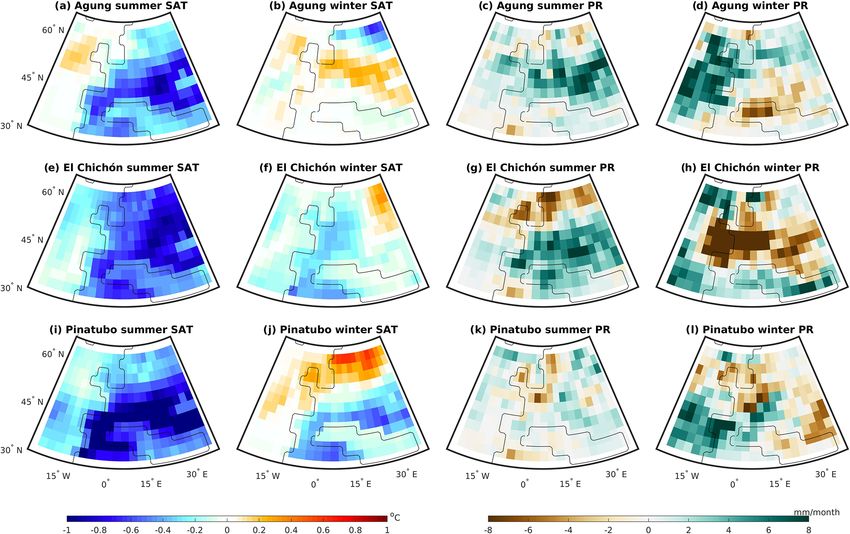
402                                                                N. Maher et al.: Large ensemble climate model simulations

1   An introduction to SMILEs                                       ment between the SMILEs for individual scientific questions.
                                                                    SMILEs from seven GCMs have now become publicly avail-
A single model initial-condition large ensemble (SMILE; see         able (Deser et al., 2020). In the reference paper for this model
Table 1 for a glossary of abbreviations) is a set of model          archive, Deser et al. (2020) have demonstrated that this col-
simulations starting from different initial conditions but pro-     lection “offers an unprecedented opportunity for evaluating
duced with a single climate model and identical external            and comparing models’ forced responses and their internal
forcing. Over the last decade SMILEs have been increasingly         variability”. Despite their recent availability these SMILEs
utilised in climate science (e.g. Zelle et al., 2005; Branstator    are already widely used. Some examples include the investi-
and Selten, 2009; Kay et al., 2015; Frankignoul et al., 2017;       gation of the role of internal variability and model differences
Kirchmeier-Young et al., 2017; Sanderson et al., 2018; Stolpe       in affecting future projections (Maher et al., 2020; Lehner
et al., 2018; Maher et al., 2019; Deser et al., 2020). The value    et al., 2020; Maher et al., 2021), trends in sea surface temper-
of SMILEs comes from the ability to quantify and separate           ature patterns (Olonscheck et al., 2020) and South American
the internal variability of the climate system and the forced       summer rainfall (Díaz et al., 2021), the decadal modulation
response to changes in external forcing (e.g. Kay et al., 2015;     of global warming (Liguori et al., 2020), the time of emer-
Maher et al., 2019). Additional value comes from identify-          gence of ocean biogeochemical trends (Schlunegger et al.,
ing and robustly sampling extreme events (e.g. heatwaves,           2020), and Arctic extremes (Landrum and Holland, 2020).
floods, and droughts), which potentially have large impacts         These SMILEs have also been investigated for use in adap-
on people despite their low probability of occurrence (e.g.         tion decision making (Mankin et al., 2020), hydroclimate un-
Fischer et al., 2013; Suarez-Gutierrez et al., 2018; Haugen         certainty in east–central Europe (Topál et al., 2020), and un-
et al., 2018). Here, SMILEs allow a more accurate sampling          certainty in projections of global land monsoon precipitation
of the entire probability distribution, including the tails of      (Zhou et al., 2020).
the distribution where extreme events occur. This sampling             GCM SMILEs have been used not just to investigate sci-
additionally allows for future projections of events with long      entific questions, they have also been utilised as test beds
return periods to be made (e.g. van der Wiel et al., 2019). Dif-    for new approaches, and tools to inform policy makers. They
ferent applications require different types of SMILEs. For ex-      have been used to create an observational large ensemble
ample, to investigate questions that involve the entire climate     (McKinnon et al., 2017; McKinnon and Deser, 2018) and
system, global climate model (GCM) SMILEs must be used.             test dynamical adjustment techniques (Deser et al., 2016;
However, to investigate impacts at local scales, regionally         Lehner et al., 2017). They have also been used to develop
downscaled climate model (RCM) SMILEs are more appro-               new methodologies such as utilising the ensemble dimension
priate. Here, we provide an overview of the exciting new sci-       for analysis (Herein et al., 2017; Maher et al., 2018, 2019;
ence published in the special issue “Large Ensemble Climate         Haszpra et al., 2020a, b) and to develop and test statisti-
Model Simulations: Exploring Natural Variability, Change            cal methods for isolating the forced response (Sippel et al.,
Signals and Impacts”. We also present a perspective on the          2020; Wills et al., 2020). Such ensembles have additionally
value of combining different types of existing SMILEs, by           provided important information for policy makers, such as
presenting four simple examples combining a GCM, RCM,               whether emission reductions are likely to be detectable in the
and a natural forcing only GCM SMILE.                               coming years, or whether they could be masked by internal
   A large body of literature already exists using individual       variability (Lehner et al., 2016; Tebaldi and Wehner, 2018;
GCM SMILEs. The majority of studies have used the Com-              Marotzke, 2019; Spring and Ilyina, 2020).
munity Earth System Model Large Ensemble (CESM-LE;                     Targeted experiments that utilise the main advantage of
Kay et al., 2015) as it has been available for the longest          SMILEs, i.e. to isolate the forced response and internal vari-
period of time (since 2015). Many studies have utilised the         ability, have also been run that both build on and comple-
power of SMILEs to investigate the internal variability of          ment the GCM studies. Some examples of such targeted ex-
the climate system (e.g. Fasullo and Nerem, 2016; Frankig-          periments include single-forcing SMILE experiments, which
noul et al., 2017; Smith and Jahn, 2019; Dai and Bloecker,          have been used for detection and attribution (e.g. Kirchmeier-
2019) and extreme events (e.g. Diffenbaugh et al., 2015; Gib-       Young et al., 2017), and RCM SMILEs, which are increas-
son et al., 2017; Kirchmeier-Young et al., 2017; Tebaldi and        ingly being used for impact studies (e.g. Leduc et al., 2016).
Wehner, 2018; Wang et al., 2018). Studies have also looked          Other complementary experiments include a large ensem-
into all components of the climate system, including the            ble which is designed to test the sensitivity of the historical
biosphere, with oceanic biogeochemistry included in these           simulations to known uncertainties in aerosol forcing (Dittus
models (e.g. Rodgers et al., 2015; McKinley et al., 2016;           et al., 2020). Atmosphere- or ocean-only large ensembles are
Lovenduski et al., 2016; Krumhardt et al., 2017; Li and Ily-        also used to quantify the internal variability in select parts
ina, 2018; Schlunegger et al., 2019). More recently studies         of the climate system when the rest of the climate system is
have utilised a combination of multiple SMILEs (e.g. Maher          fixed to observed values (Gates, 1992; Barnett et al., 1997;
et al., 2018; Fasullo et al., 2020; Schlunegger et al., 2020;       Penduff et al., 2014). In the following paragraphs we outline
Zhou et al., 2020), allowing the assessment of model agree-         the utility of some of these targeted experiments, focusing on

Earth Syst. Dynam., 12, 401–418, 2021                                                  https://doi.org/10.5194/esd-12-401-2021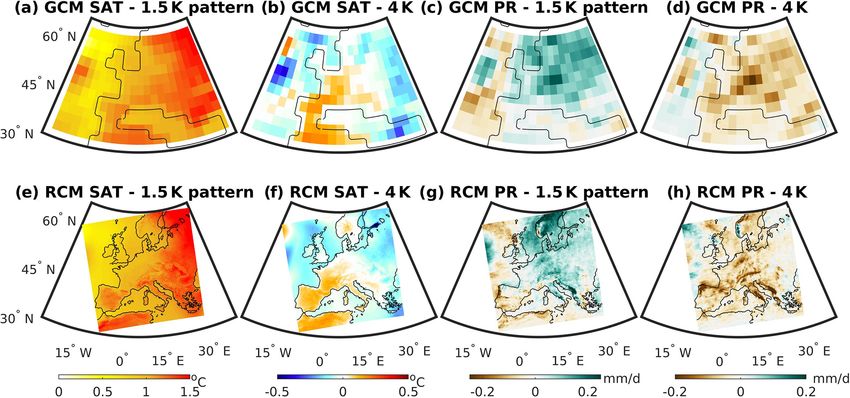
N. Maher et al.: Large ensemble climate model simulations                                                                               403

Table 1. Glossary of acronyms presented in alphabetical order for three categories: large ensemble types, Earth system acronyms, and specific
climate models and modelling projects.

    large ensemble types
    GCM                  global climate model; a model of the Earth system that encompasses the entire globe and includes ocean,
                         atmosphere, land, and ice components
    nat-GCM              GCM forced by natural forcing only; i.e. does not have greenhouse gas or anthropogenic aerosol forcing
    RCM                  regionally downscaled climate model; high-resolution climate model of a portion of the globe with its bound-
                         aries set using GCM output
    SMILE                single model initial-condition large ensemble; a set of model simulations starting from different initial condi-
                         tions but produced with a single climate model and identical external forcings
    Earth system acronyms
    DJF                  boreal winter mean taken over December, January, February
    ENSO                 El Niño–Southern Oscillation
    JJA                  boreal summer mean taken over June, July, August
    max-SAT              maximum daily surface air temperature
    NAO                  North Atlantic Oscillation
    SAT                  surface air temperature
    SEOF                 snapshot empirical orthogonal function
    SST                  sea surface temperature
    Specific climate models and modelling projects
    CanESM2              Canadian Earth System Model (Second Generation) used as part of the Canadian Earth System Model Large
                         Ensembles and as boundary conditions for CRCM5-LE (Kushner et al., 2018; Kirchmeier-Young et al., 2017)
    CESM-LE              Community Earth System Model Large Ensemble (Kay et al., 2015)
    ClimEx               regional large ensemble project; uses CRCM5 with CanESM2 as the boundary conditions for CRCM5-LE
                         (Leduc et al., 2019)
    CMIP                 Coupled Model Intercomparison Project
    CRCM5                Canadian Regional Climate Model, used in the CRCM5-LE (Martynov et al., 2013)
    CRCM5-LE             Canadian Regional Climate Model Large Ensemble; part of the ClimEx experiment
    EURO-CORDEX          Coordinated Downscaling Experiment – European Domain
    LAERTES-EU           Large Ensemble of Regional Climate Model Simulations for Europe (Ehmele et al., 2020)
    MIROC5               Model for Interdisciplinary Research on Climate version 5 (Watanabe et al., 2010)
    MPI-GE               Max Planck Institute Grand Ensemble (Maher et al., 2019)

single-forcing and RCM ensembles as these are able to ex-                solar) forcing. These experiments were completed for the
plore a wide range of possible past and future states as they            period 1950–2020. The Canadian large ensemble has been
include all components of the climate system.                            used to show that extreme fire events in Canada are 1.5 to
   Single-forcing SMILEs are used to separate the role of dif-           6 times more likely under anthropogenic greenhouse gas
ferent forcings and to attribute change to different drivers.            forcing compared to a climate with natural forcing alone
The first single-forcing SMILE was run as part of the Cana-              (Kirchmeier-Young et al., 2017). This ensemble has been
dian large ensemble experiments (Kirchmeier-Young et al.,                used to show that anthropogenic aerosols offset the effects
2017). This ensemble consists of a GCM run for 50 mem-                   of anthropogenic greenhouse gases on ice cover in the mid-
bers with all forcings, 50 members with only anthropogenic               twentieth century (Gagné et al., 2017a) and that large vol-
aerosols, and 50 members with only natural (volcanic and                 canic eruptions result in an increase in Arctic sea ice follow-

https://doi.org/10.5194/esd-12-401-2021                                                       Earth Syst. Dynam., 12, 401–418, 2021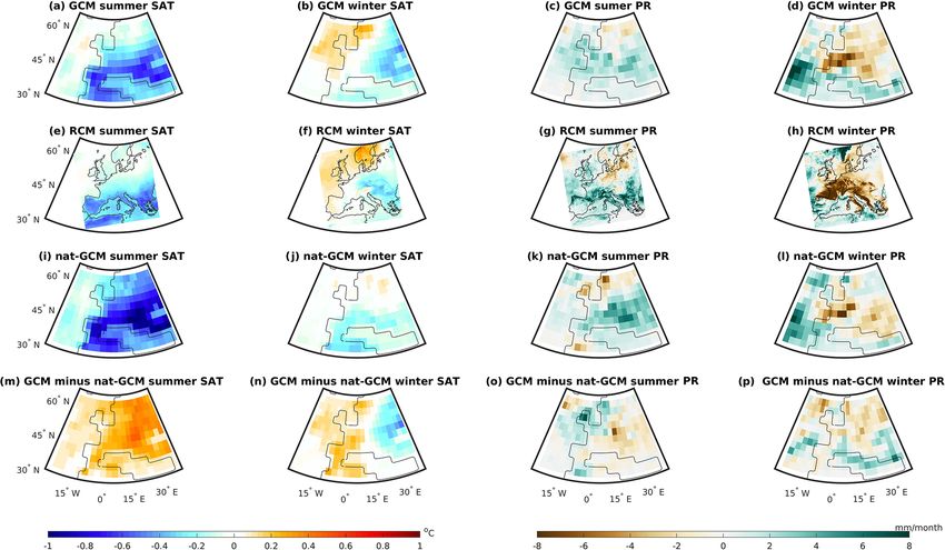
404                                                                N. Maher et al.: Large ensemble climate model simulations

ing the eruption (Gagné et al., 2017b). This single-forcing         et al., 2019). They can also be used to look at local changes
SMILE has also been used in combination with another                in internal variability (e.g. Leduc et al., 2019) and projected
SMILE (CESM-LE) to investigate the detection timescale of           changes in the signal-to-noise ratio of both the mean and
tropospheric warming in single-ensemble members (Santer             importantly extremes (Aalbers et al., 2018; Poschlod et al.,
et al., 2019). Here, the authors provided an estimate as to         2020b). With the availability of SMILEs, impact studies, e.g.
how uncertainty due to internal variability can affect the time     in hydrology, can assess new ways of analysing the impacts
required to detect patterns of change and how dependent this        of climate change on hydrological processes, reaching from
detection time is on different types of forcing from the single-    water balance studies and flow regime changes (Poschlod
forcing simulations.                                                et al., 2020a) to extreme events, such as floods (Willkofer
   A different type of single-forcing SMILE has also been run       and Ludwig, 2020). In order to deal with the challenges of
where an individual forcing is set to a specific value but all      dynamically altered extreme events under climate change,
others remain as in the full experiment as opposed to fixing        often compound events, SMILEs can introduce the concept
all but one forcing as in the Canadian large ensemble (Pen-         of analysing the relevance of climate variability by means
dergrass et al., 2019). By keeping aerosols fixed at the pre-       of spatially explicit and process-based models, assessing the
industrial level Pendergrass et al. (2019) are able to identify     non-linear response to multiple meteorological drivers, such
the relationship between global warming and extreme pre-            as in alpine snow cover dynamics (Willibald et al., 2020) and
cipitation. Previous studies have assumed that single-forcing       (managed) land surface responses (Zscheischler et al., 2018).
experiments can be linearly added to recreate an all-forcing        SMILEs can be used as new instruments to provide the data
experiment result. Pendergrass et al. (2019) find that the re-      density and the parameter space to deal with the high pro-
lationship in their model is quadratic and stress that the re-      cess complexity and (often) data scarcity, especially when
sponse of extreme precipitation to aerosols is state dependent      operational flood forecasting or flood risk management is tar-
and as such the linearity assumption that is often used in the      geted (Willkofer and Ludwig, 2020). For all of these cases,
context of single-forcing experiments does not hold for this        SMILEs can serve as a provider of coherent and standardised
quantity. These results demonstrate the need for many dif-          data, providing a very useful extension to the existing top–
ferent types of experiment to answer different questions and        down modelling chain concepts, by enabling the application
show that when there is large internal variability these exper-     of artificial intelligence, machine learning, and big data con-
iments must be run as large ensembles.                              cepts for impact studies.
   RCMs allow for higher-resolution studies and smaller-               Given the recent availability of many of the aforemen-
scale impact-based studies than GCMs. Internal variability          tioned tools, SMILEs are currently only beginning to be
is found to be larger at smaller spatio-temporal scales (Aal-       utilised to their full power. There are unexploited opportu-
bers et al., 2018) demonstrating the need for RCM SMILEs            nities for a wide range of disciplines, such as hydrology, bio-
that can resolve these scales and provide a large sample size       geosciences, and climate dynamics. The special issue “Large
(Wood and Ludwig, 2020). RCMs have the advantage the                Ensemble Climate Model Simulations: Exploring Natural
they can better represent local values. For example Leduc           Variability, Change Signals and Impacts” was open to sub-
et al. (2019) found a better representation of extreme tem-         missions which exploited these new opportunities and ex-
perature and precipitation locally in an RCM SMILE com-             plored how a combined analysis of the different types of ex-
pared to its driving GCM SMILE. In applying machine learn-          isting large ensembles can advance our knowledge in differ-
ing techniques, RCM SMILEs were of great service to de-             ent fields. Submissions were particularly invited to use new
tect frequencies, intensities, and the temporal dynamics of         methods to investigate these topics. The new contributions
Vb cyclones (a specific type of cyclone associated with ex-         published in this special issue will be summarised in the fol-
treme precipitation and flooding over Europe) and the asso-         lowing section.
ciated patterns of extreme precipitation over central Europe
(Mittermeier et al., 2019). Multiple RCM SMILEs are now
becoming available (e.g. Aalbers et al., 2018; Leduc et al.,        2   Advances in knowledge from this special issue
2019; Kirchmeier-Young et al., 2019; Lang and Mikolajew-
icz, 2020), which are currently run over European and North         The nine studies published in “Large Ensemble Climate
American domains. Having multiple RCM SMILEs is im-                 Model Simulations: Exploring Natural Variability, Change
portant as different RCMs have different magnitudes of inter-       Signals and Impacts” have utilised a wide range of types
nal variability. This was demonstrated by von Trentini et al.       of SMILEs including seven GCM SMILEs, three RCM
(2019), who found that internal variability of a single RCM         SMILEs, hydrological models driven by RCMs, a SMILE
SMILE covers some but not all of the spread in a multi-model        for event attribution (prescribed sea surface temperature), a
RCM ensemble.                                                       data-assimilated SMILE, and an initialised regional SMILE.
   Large ensembles of RCMs are currently used for a vari-           As such the studies published in this special issue cover a
ety of purposes. They can be used for event attribution at          wide range of SMILEs that can be used for a variety of pur-
higher-resolution scales than GCMs (e.g. Kirchmeier-Young           poses. The studies fall into the following categories: (1) novel

Earth Syst. Dynam., 12, 401–418, 2021                                                  https://doi.org/10.5194/esd-12-401-2021
N. Maher et al.: Large ensemble climate model simulations                                                                      405

methods, (2) RCM large ensemble evaluation and use, and            “An investigation of weighting schemes suitable for incorpo-
(3) impacts of global warming. They will be presented in the       rating large ensembles into multi-model ensembles”. They
following sections.                                                provide a comprehensive explanation of how one would de-
                                                                   termine weights for any application and demonstrate that rea-
Novel methods
                                                                   sonable weights can be generated when taking both model
                                                                   performance and independence into account. Having such a
Four novel methodologies have been published in this special       methodology that allows the use of all available information
issue. The study of Haszpra et al. (2020a) entitled “Investi-      is highly valuable and will be applicable as the new CMIP6
gating ENSO and its teleconnections under climate change in        data becomes available. Due to its importance for upcoming
an ensemble view – a new perspective”, uses a single GCM           analyses of the CMIP6 simulations this article was published
SMILE (CESM-LE) and the snapshot empirical orthogonal              in ESD’s highlight section.
function (SEOF) analysis method to investigate the El Niño–           With the recent availability of many SMILEs, which vary
Southern Oscillation (ENSO) pattern and amplitude changes          in size from as few as 15 members to as many as 200
in each individual season by applying an SEOF across the en-       members, it is now important to ask the following question:
semble for each month of the year. Haszpra et al. (2020a) are      “How large does a large ensemble need to be?”. Milinski
then able to investigate teleconnections of ENSO (taken as         et al. (2020) do this, presenting a method to estimate the re-
the first principal component) with precipitation data by com-     quired ensemble size for any given problem using a single
puting lagged regressions between the two variables. The           GCM SMILE (Max Planck Institute Grand Ensemble; MPI-
use of this methodology has allowed Haszpra et al. (2020a)         GE) and a long pre-industrial control simulation to test the
to identify an increase in the sea surface temperature (SST)       method. They demonstrate that the required ensemble size
fluctuations in the ENSO region that is most pronounced in         depends on both the question asked and the acceptable error
June, July, August, and September but also occurs in Decem-        to the user. In general the signal (response to external forcing)
ber, January, and February. They have also used this method-       and the magnitude of the internal variability determine how
ology to identify which ENSO teleconnections are projected         large the ensemble needs to be. The smallest ensemble size
to change and to become more pronounced in this SMILE.             is needed for estimating the forced response, with a larger
For example they find enhanced positive precipitation cor-         size needed to quantify internal variability and the highest
relations with ENSO in central Africa and on the western           ensemble size required to detect changes in internal variabil-
coast of South America and a more pronounced anticorrela-          ity. They also demonstrate that more members are needed
tion over Australia and the southern edge of South America         for regional than global quantities. This method can be used
that occur in June, July, August, and September.                   by any scientist to identify the ensemble size required before
   Hawkins and Sutton (2009) originally proposed a method-         starting their study.
ology to partition uncertainty into that from model differ-           These novel methodologies demonstrate the utility of
ences, internal variability, and scenario choices using a multi-   SMILEs as a test bed and show that when using SMILEs
model ensemble. Lehner et al. (2020) revisit this methodol-        traditional methods can be redefined and new methods de-
ogy in a study entitled “Partitioning climate projection uncer-    veloped, which exploit the power of large ensembles.
tainty with multiple large ensembles and CMIP5/6”. Here,
using seven GCM SMILEs and the Coupled Model Inter-                RCM large ensemble evaluation and use
comparison Projects 5 and 6 (CMIP5 & 6), they show that the
original approach works well at global and regional scales;        RCM SMILEs have been used extensively in this special is-
however, for local scales a more accurate partitioning of un-      sue with two studies specifically evaluating how well RCMs
certainty is needed, which can only be achieved using the          perform. Böhnisch et al. (2020) use the 50-member Canadian
SMILEs. They additionally demonstrate that differences be-         Regional Climate Model Large Ensemble (CRCM5-LE) to
tween CMIP5 and 6 can to some extent be reconciled by nor-         investigate the regional response to the North Atlantic Os-
malising projections by global mean temperature or applying        cillation (NAO). In particular, they investigate how well the
a simple model weighting that targets high climate sensitiv-       NAO signal propagates from the GCM domain to the RCM
ities. This shows that the differences between CMIP5 and 6         domain in a study entitled “Using a nested single model large
results are largely due to the high climate sensitivities found    ensemble to assess the internal variability of the North At-
in some of the CMIP6 models.                                       lantic Oscillation and its climatic implications for Central
   With the newly available CMIP6 data, where some mod-            Europe”. They find that both models reproduce the NAO pat-
els have one ensemble member and some models have many,            tern, with the large-scale NAO propagating properly into the
the question of how to combine these data in the most mean-        finer-scale RCM domain; however, the RCM produces more
ingful way has been asked. Merrifield et al. (2020) use three      realistic spatial climate patterns, likely due to the additional
GCM SMILEs and 88 members of CMIP5 to provide a com-               topographic features. These features in the RCM are also
prehensive evaluation of five different weighting strategies       found to provide value in evaluating regional NAO impacts,
for a multi-model ensemble that includes some SMILEs in            with the relationship between the NAO and climate over Eu-

https://doi.org/10.5194/esd-12-401-2021                                                Earth Syst. Dynam., 12, 401–418, 2021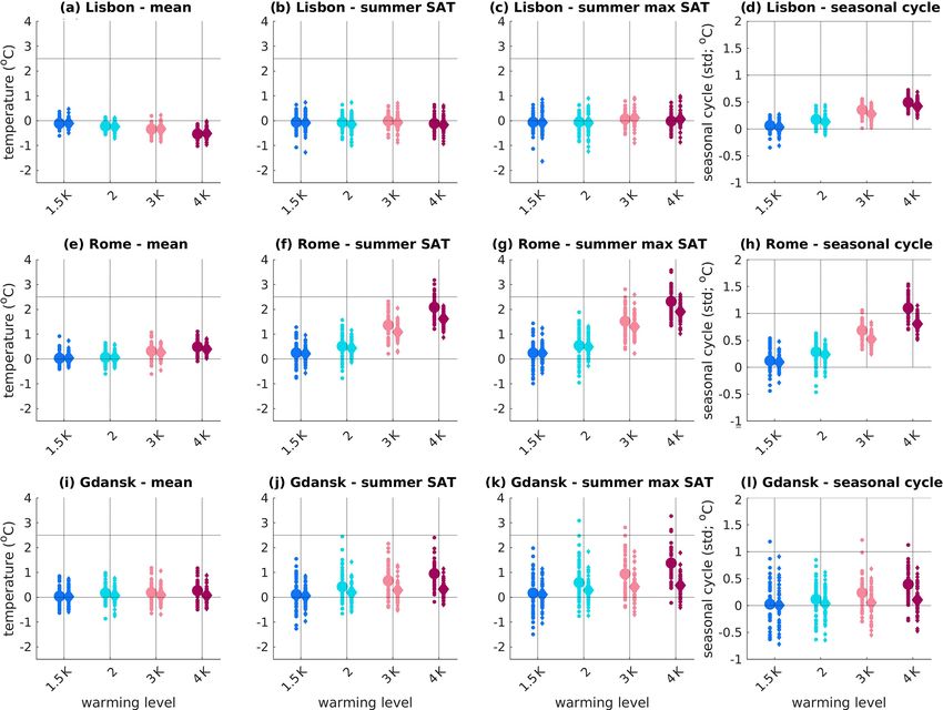
406                                                                N. Maher et al.: Large ensemble climate model simulations

rope predicted to slightly weaken in the future. This study         warm events associated with high flows particularly in the
highlights how dynamically downscaling a GCM SMILE can              vicinity of Lake Erie, especially when there are high 500mb
help to understand regional impacts of major modes of inter-        geopotential height anomalies centred on the eastern Great
nal variability by combining the advantages of a large sample       Lakes and the Atlantic Ocean. Using the RCM SMILE they
size with high resolution to represent regional processes.          are able to investigate how the internal variability of climate
   A multi-RCM SMILE comparison over Europe was pro-                will modulate the future evolution of these hydrometeoro-
vided by von Trentini et al. (2020). They compare three RCM         logical extremes and show that the increase in events can be
SMILEs with observations in “Comparing interannual vari-            amplified or attenuated depending on the location of pressure
ability in three regional single model initial-condition large      systems modulated by internal variability.
ensembles (SMILEs) over Europe”. This study evaluates sea-             Ehmele et al. (2020) use a single RCM SMILE (Large
sonal temperature, precipitation, dry periods, and heatwaves.       Ensemble of Regional Climate Model Simulations for Eu-
They find that the three ensembles agree well with observa-         rope; LAERTES-EU) that consists of both long-term and ini-
tions for interannual variability and that despite some model       tialised simulations as well as runs that assimilate reanalysis
differences, the sign of projected future variability changes is    data to look at “Long-term variance of heavy precipitation
similar across models. Specifically, they find an increase in       across central Europe using a large ensemble of regional cli-
summer temperature and precipitation variability as well as         mate model simulations”. They find that the model represents
decreases in winter temperature and precipitation variability       observed extreme precipitation well. When considering fu-
under strong global warming. They also find increased vari-         ture projections, the upcoming decade shows a continuation
ability in summer in the number of heatwaves and the maxi-          of past tendencies in Mid-Europe, with increasing heavy pre-
mum length of a dry period in two of the three models. The          cipitation, with no clear signal for the Alps. Additionally they
study highlights the differences in projected interannual vari-     use the power of the large ensemble to show that there are
ability between ensemble members and shows that SMILEs              phases of increased and decreased heavy precipitation that
are necessary to robustly quantify the significance of such         are due to internal variability alone. Generally, they empha-
changes.                                                            sise the benefit of RCM SMILEs for an improved estimation
   These two studies – Böhnisch et al. (2020) and von Tren-         of extreme values, building on robust statistics.
tini et al. (2020) – have both demonstrated the value of using         A large event attribution ensemble (Model for Interdisci-
an RCM SMILE in addition to a GCM SMILE (Böhnisch                   plinary Research on Climate 5; MIROC5), where sea surface
et al., 2020) and provided some confidence in projections           temperatures and ice are prescribed, is used to demonstrate
across the European domain (von Trentini et al., 2020).             the role of historical anthropogenic warming on droughts
                                                                    and fires in equatorial Asia (Shiogama et al., 2020). In the
Impacts of global warming
                                                                    study entitled “Historical and future anthropogenic warm-
                                                                    ing effects on droughts, fires and fire emissions of CO2 and
Many studies in this special issue address the changing prob-       PM2.5 in equatorial Asia when 2015-like El Niño events oc-
abilities of extreme events and their impacts under a chang-        cur”, Shiogama et al. (2020) show significant increases in
ing climate. SMILEs are the perfect tool to investigate such        burned area, carbon dioxide, and PM2.5 emissions at 1.5 and
events because they sample the probability distribution at          2 ◦ C of warming, with the chance of exceeding the large 2015
each time step and allow assessment of changes in the proba-        event reaching 100 % under 3 ◦ C of warming. They also ar-
bilities of events such as floods, droughts, and heatwaves. In      gue for including fires in future climate modelling scenarios
this special issue Canadian winter hydrometeorological ex-          as these can affect global carbon dioxide emissions.
treme events are investigated by Champagne et al. (2020),              Finally the previously discussed papers of Böhnisch et al.
European flooding events are investigated by Ehmele et al.          (2020) and Haszpra et al. (2020a) also investigate impacts
(2020), and fire and drought in Asia are investigated by Sh-        of the modes of variability: NAO and ENSO respectively.
iogama et al. (2020).                                               Böhnisch et al. (2020) find an increasing the frequency of
   Champagne et al. (2020) published “Winter hydromete-             a negative NAO that favours colder and harsher winters in
orological extreme events modulated by large-scale atmo-            Europe. Haszpra et al. (2020a) demonstrate that some ENSO
spheric circulation in southern Ontario”. In this study they        teleconnections can change, with some increasing in strength
use a single RCM SMILE (CRCM5-LE) to create a new                   while others decrease, which will have different impacts in
winter compound index to investigate the contribution of the        different regions. An example of the changes they find is an
combination of rain and snowmelt to extreme events. They            increase in precipitation teleconnections between ENSO and
then use the output from the RCM SMILE as input to a hy-            Australia and Africa in their respective winters at the end of
drological model to identify the necessary conditions needed        the century.
for high flows to occur in three southern Ontario watersheds           Overall these studies on changing events and their impacts
and to project their future evolution. They find that the RCM       are made possible by the use of SMILEs, where extreme
output is realistic when compared to observational data and         events are well sampled and changes in modes of variability
project an increase in the future number of heavy rain and          can be separated from large internal variability. These stud-

Earth Syst. Dynam., 12, 401–418, 2021                                                  https://doi.org/10.5194/esd-12-401-2021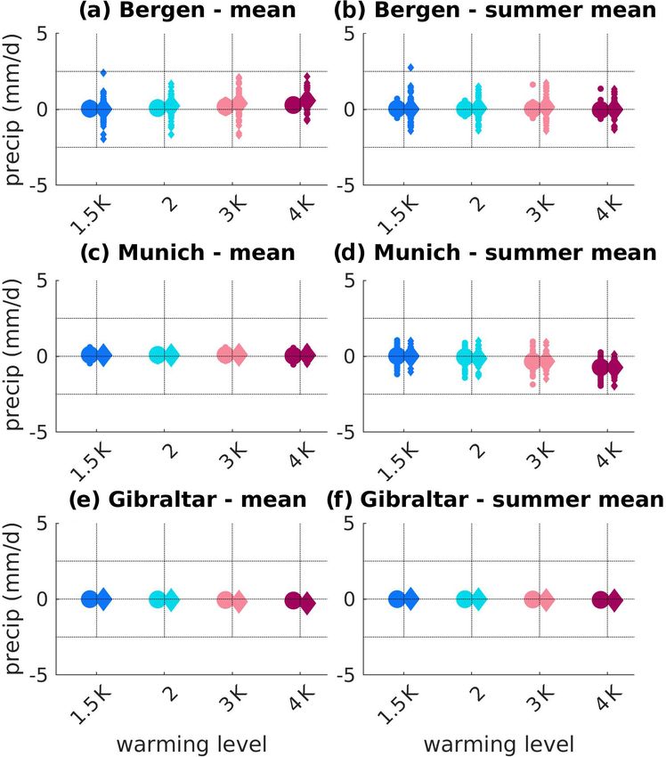
N. Maher et al.: Large ensemble climate model simulations                                                                    407

ies are relevant for policy and planning, with Ehmele et al.        as the average of June, July, and August (JJA) and winter as
(2020) demonstrating high variability in precipitation over         the average of December, January, and February (DJF).
different decades in Europe, Champagne et al. (2020) show-             The ensemble mean SAT and precipitation at 1 K of warm-
ing changes in flood risk in Ontario in their study, and Sh-        ing are shown for the GCM and RCM SMILEs in Fig. 1.
iogama et al. (2020) finding an increase in the risk of large       The continental outlines highlight the resolution difference
fires and their impacts in equatorial Asia under increasing         between the GCM and the RCM. The patterns of both SAT
warming.                                                            and precipitation are broadly similar between the GCM and
                                                                    the RCM, with warmer temperatures to the south and more
                                                                    precipitation to the north-west of the domain, particularly
3   Perspectives on new tools and their value                       over the United Kingdom and western Norway. Figure 1 also
                                                                    shows that the increased resolution of the RCM allows the
There are now many SMILEs available for use in the climate          local patterns to be better resolved and highlights the ef-
community. These include GCM SMILEs, atmosphere- and                fects of features such as coastlines and mountains. Subtract-
ocean-only SMILEs, single forced SMILEs, SMILEs forced              ing the GCM from the RCM shows that the RCM tends to
with all except one forcing, RCM SMILEs, and SMILE                  be slightly cooler and wetter than the GCM. While there
experiments with different sets of forcing such as vary-            has been no comprehensive validation of whether the GCM
ing aerosols. In this section we present some simple exam-          or RCM is more realistic, when compared to observations
ples to investigate the value of combining different types of       over Europe, Leduc et al. (2019) found a better represen-
SMILEs and demonstrate how future research can benefit              tation of extreme precipitation and local extremes in the
from using the SMILEs which are already available. To do            RCM than the GCM, particularly over coastal and moun-
this we use the Canadian Earth System Model Large En-               tain regions, due to the higher resolution. In general due to
semble (CanESM2; Kirchmeier-Young et al., 2017; Kush-               their higher-resolution RCMs provide a more realistic rep-
ner et al., 2018) because it has 50 members of both the full        resentation of smaller scales, such as land–sea contrasts and
forced ensemble (1950–2100; historical and RCP8.5) and 50           orography and, at higher resolutions, lakes and rivers (e.g.
members of natural-only forcing (solar and volcanic forc-           Lucas-Picher et al., 2017; Rummukainen, 2010; Christensen
ing; 1950–2020). These SMILEs are henceforth referred to            and Kjellström, 2020; Feser et al., 2011). This makes RCMs
as GCM and nat-GCM. We combine the GCM and nat-GCM                  more suited for looking at impacts at local scales and more
with the Canadian Regional Climate Model Large Ensem-               reliable than GCMs when looking at small regions and events
ble (CRCM5-LE as part of the ClimEx project; Leduc et al.,          on shorter timescales (Rummukainen, 2016).
2019), which uses the Canadian Regional Climate Model                  To demonstrate the utility of combining different types of
(12km resolution CRCM5; Martynov et al., 2013; Šeparović           SMILE we consider the following simple examples:
et al., 2013) with the CanESM2 GCM SMILE with all forc-
ings used as boundary conditions. We utilise the European            1. We ask whether the SAT and precipitation responses
domain from this SMILE. This SMILE will be referred to as               over Europe are linear with global warming in both the
RCM for the rest of this study.                                         GCM and RCM.
   To investigate the value of combining the GCM and RCM
                                                                     2. We investigate SAT, max-SAT, and precipitation projec-
SMILEs we will evaluate changes in both near-surface air
                                                                        tions in a subset of European cities in both the GCM and
temperature (SAT) and precipitation at multiple warming lev-
                                                                        RCM at 1.5, 2, 3, and 4 K global warming. These cities
els. The warming levels are 1 K (2002), 1.5 K (2015), 2 K
                                                                        are shown in Fig. 1 and are chosen due to their location
(2028), 3 K (2048), and 4 K (2067). The years at which each
                                                                        near the coastline or in mountainous regions, where the
warming level occurs are found using the ensemble mean
                                                                        increased resolution of the RCM may provide additional
from the GCM as compared to the pre-industrial control. We
                                                                        information.
use an 11-year window centred on each warming level to
analyse the data. Projected changes are always shown relative        3. We investigate whether there are forced changes and, if
to the 1 K level (similar to the present day; Allen et al., 2018)       so, their drivers in summer SAT variability at 1.5 and
and are computed individually for each ensemble member.                 4 K, by combining the GCM, nat-GCM, and RCM
This choice allows us to investigate future changes above the
present day. This is particularly relevant in light of the tar-      4. Finally we investigate the European seasonal response
gets of 1.5 and 2 K set by the Paris Agreement. In addition             to large volcanic eruptions using all three SMILEs.
to SAT and precipitation we use the variable maximum daily
temperature (tasmax in the ensemble output), henceforth re-         Regional response to global warming
ferred to as max-SAT. For the GCM this variable is output
as the monthly mean of the daily maximum temperature. We            In this section we ask whether the European SAT and precipi-
average the daily data from the RCM to be comparable. For           tation responses are linear with global warming. By using the
the analyses presented in this editorial summer is computed         GCM SMILE we can pinpoint specifically when the model

https://doi.org/10.5194/esd-12-401-2021                                               Earth Syst. Dynam., 12, 401–418, 2021
408 N. Maher et al.: Large ensemble climate model simulations
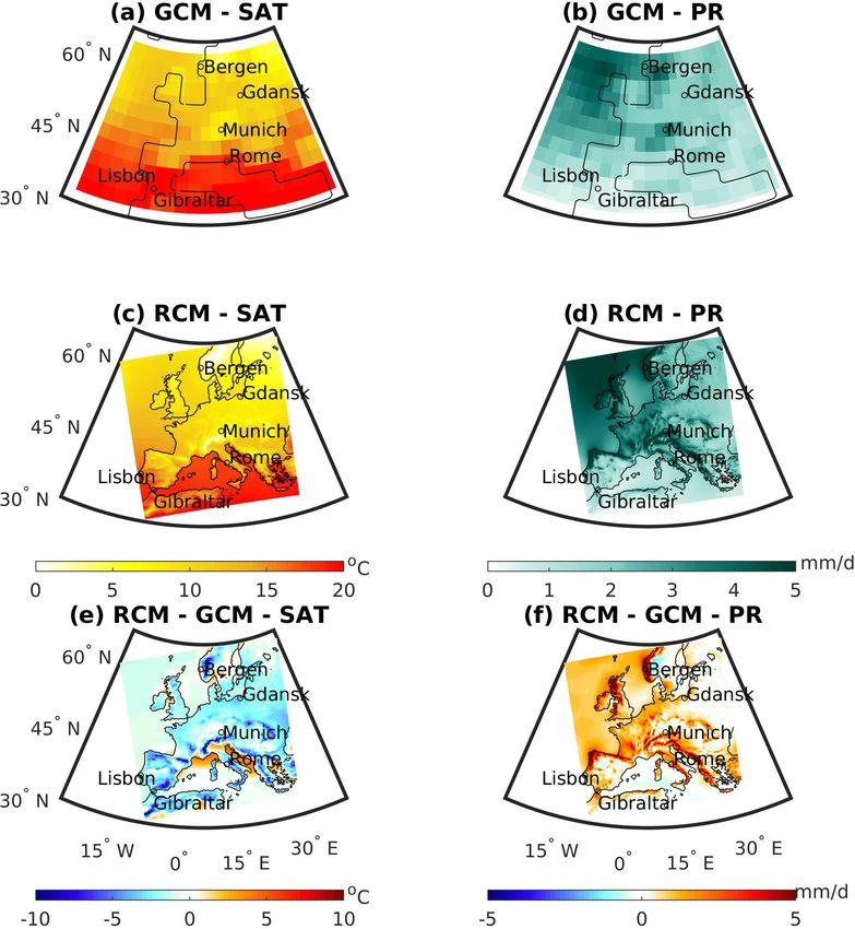
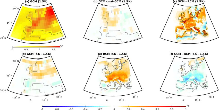
non-linearity. When considering precipitation, the response
is again non-linear (Fig. 2d, h), with the increase in precip-
itation over northern Europe not as large at 4 K as at 1.5 K,
but the decrease over southern Europe larger. While there is
agreement between the GCM and RCM on the broad-scale
pattern, the RCM is needed to resolve the local precipitation
non-linearity and the response over southern Europe. The re-
sult that there is more added value of the RCM for precipi-
tation than SAT is in agreement with previous work as pre-
cipitation is more affected by orography and small-scale pro-
cesses than SAT (Lucas-Picher et al., 2017; Christensen and
Kjellström, 2020; Feser et al., 2011; Rummukainen, 2016).
Projections in individual European cities
Given that the RCM provides the most additional informa-
tion at local scales, particularly near the coastlines and orog-
raphy, we next investigate some major cities across Europe
(shown in Fig. 1), all of which are near the coastline or orog-
raphy. Here, we investigate how the warming in an individual
city compares to the global mean warming by utilising the
power of the SMILEs and computing the forced response in
Figure 1. Ensemble mean surface air temperature (SAT) and pre- each city. For example if we take a city such as Rome, we can
cipitation in the GCM (a, b) and RCM (c, d) SMILEs over Eu- ask the question of whether we expect Rome to warm more
rope at 1 K warming (2002). The difference between the RCM and or less than the global mean. We can then ask whether this
GCM SMILEs is shown in (e) and (f). We use an 11-year window relative warming is linear with global warming; i.e. if at 2 K
around the warming year to analyse the data. The cities investigated warming Rome warms more than the global mean, does it
in Figs. 3 and 4 are shown on the maps. Continental borders are warm the same amount more at 4 K? Finally because we are
plotted for each model’s native grid. using SMILEs we can look at the range of warming in Rome
that we could observe due to internal variability. For example
if the mean warming is the same as the global mean warm-
has reached a given level of global warming. By computing ing, how much more or less warming than the mean could
the ensemble mean at each warming level, we can precisely we observe due to internal variability? Here, we will assess
identify the forced response at each warming level in both the if the answers to these questions differ between the GCM and
GCM and RCM. Due to the large ensemble sizes, differences RCM.
between the GCM and RCM can be directly attributed to dif- We find a range of results across the three cities (Fig. 3).
ferences in the forced response between the two SMILEs. When we consider the ensemble mean warming, Lisbon
Using an RCM for climate projections has previously been warms less than the global mean, while Rome warms slightly
shown to both provide additional value, but to also introduce more and Gdańsk warms similarly. Rome and Gdańsk warm
additional biases (Jacob et al., 2020). The added value has more in summer and in the summer maximum temperature
been shown to come from better representation of physical than the global mean, especially at larger levels of warming.
mechanisms as well as the better representation of underly- This means that someone living in these cities would likely
ing topography (Dudhia, 2014; Mearns et al., 2013; Di Luca experience more warming than the global mean level would
et al., 2013; Evans and McCabe, 2013), suggesting the RCM suggest. Surprisingly, we find that the RCM shows less non-
projections may be regionally more reliable than the GCM. linearity in the relative warming than the GCM. This gives
We find that the scaled SAT and precipitation patterns at slightly lower projected temperatures and a slightly more
1.5 K are very similar in the GCM and RCM (Fig. 2a, c, e, g). promising outlook when using the RCM as compared to the
These patterns also resemble those found in the Coordinated GCM.
Downscaling Experiment in the European Domain (EURO- We next consider the seasonal cycle. Here, an increase
CORDEX) experiment (Jacob et al., 2018). By looking at means that summer warms more than winter. The seasonal
the scaled 4 K response as compared to the scaled 1.5 K re- cycle increases in Lisbon and Rome. This change and the
sponse (Fig. 2b, f), we find that the SAT response is slightly internal variability of the change are slightly smaller in the
non-linear with south-western Europe warming more at 4 K RCM than the GCM, suggesting that the local range of pos-
and northern and eastern Europe warming less relative to the sible observed changes could be smaller than expected from
scaled 1.5 K response. The RCM and GCM agree well on this the GCM. Where the internal variability no longer crosses the
Earth Syst. Dynam., 12, 401–418, 2021 https://doi.org/10.5194/esd-12-401-2021N. Maher et al.: Large ensemble climate model simulations 409
Figure 2. Surface air temperature (SAT) and precipitation change over Europe scaled by the globally averaged SAT change. (a) Scaled SAT
change at 1.5 K in the GCM, (b) scaled SAT change at 4 K with scaled SAT change at 1.5 K subtracted in the GCM, (c) scaled precipitation
change at 1.5 K in the GCM, (d) scaled precipitation change at 4 K with scaled SAT change at 1.5 K precipitation in the GCM, (e) Scaled SAT
change at 1.5 K in the RCM, (f) scaled SAT change at 4 K with scaled SAT change at 1.5 K subtracted in the RCM, (g) scaled precipitation
change at 1.5 K in the RCM, and (h) scaled precipitation change at 4 K with scaled SAT change at 1.5 K precipitation in the RCM. Changes
are computed relative to the pattern at 1 K of global warming. Continental borders are shown for the each model’s native grid. The scaled
changes in panels (a) and (d) are computed as the pointwise SAT at 1.5 K minus the pointwise SAT at 1 K dived by the global mean warming
above 1 K (i.e. 0.5 K) in each individual ensemble member. The patterns in (b) and (f) use the same calculation at 4 K, with the patterns from
(a) and (e) subtracted from them. The ensemble mean is taken prior to the subtraction. The same process is computed in the right-hand panels
for precipitation.
zero line (e.g. 3–4 K warming for Rome and Lisbon), we ex- Insights into forced changes in temperature variability
pect to see an increase in the seasonal cycle in all members,
Using SMILEs we are now able to quantify changes in in-
although the magnitude of the change depends on how the
ternal variability at different warming levels. This was not
system evolves in each individual member. This is an impor-
previously possible with single runs of climate models. By
tant advantage of using SMILEs as we can assess the range of
pooling the summer data for all ensemble members for the
possible futures that could be observed due to the combina-
11-year window around each warming level we can calculate
tion of increasing greenhouse gases and internal variability.
the internal variability at each grid point in the European do-
Finally we investigate how precipitation is projected to
main for each individual warming level. To do this we take a
change in a city on the coastline with high mean precipitation
standard deviation across the pooled data. Figure 5 shows the
(Bergen, Fig. 4a, b), a city on the coastline with low mean
GCM summer SAT internal variability at 1.5 K and the dif-
precipitation (Gibraltar, Fig. 4e, f), and a city surrounded by
ference between the GCM and the RCM and the nat-GCM.
high orography (Munich, Fig. 4c, d). We find limited changes
We find that the GCM has slightly less variability over north-
in the forced response for both mean and summer precipita-
western Europe as compared to the nat-GCM, suggesting that
tion in all three cities as compared to the precipitation at 1 K
summer variability at 1.5 K is decreased over this region as
of warming. There is little difference in the mean changes be-
compared to natural unforced variability alone. The RCM
tween the GCM and RCM. However, the RCM can have very
generally has less variability than the GCM, which indicates
different internal variability than the GCM. We find larger
that the GCM might overestimate summer SAT variability
variability in the RCM over Bergen. This means that while
over Europe. We then consider the change in variability at
there is little mean change in Bergen, at any warming level
4 K as compared to 1.5 K in both the GCM and RCM. We
the city could observe a 2.5 mm/d decrease or 3 mm/d in-
find a projected increase in variability over all of the Euro-
crease in both the mean and summer mean precipitation in
pean land mass, except Portugal and Spain, that is larger in
any given year due to internal variability alone. This demon-
the RCM than the GCM. This tells us that local processes in
strates the additional value of an RCM SMILE in planning
the RCM result in a larger increase in summer temperature
for potential observed changes in local locations.
variability, although the overall increase in both the RCM
and GCM displays the same pattern.
https://doi.org/10.5194/esd-12-401-2021 Earth Syst. Dynam., 12, 401–418, 2021410 N. Maher et al.: Large ensemble climate model simulations
Figure 3. Annual-mean surface air temperature (SAT) (a, e, i), summer SAT (b, f, j), and summer max-SAT (c, g, k) and the seasonal cycle
change (d, h, l) shown at each warming level relative to 1 K of global warming. Shown for the GCM (circles) and the RCM (diamonds).
Each ensemble member is shown in the small symbols with the ensemble mean in the large symbol. Shown for (a–d) Lisbon (38.7223◦ N,
9.1393◦ W), (e–h) Rome (41.9028◦ N,12.4964◦ E), and (i–l) Gdańsk (54.3520◦ N, 18.6466◦ E). Each ensemble members change is computed
relative to itself at 1 K, with the global warming above 1 K then subtracted for all variables except the seasonal cycle. The seasonal cycle is
computed as the standard deviation over all 12 months after the 11-year period has been averaged.
Attributing climate responses to volcanic eruptions factors such as anthropogenic emissions is. The volcanic
cooling is underestimated in the GCM and RCM SMILEs
By combining the GCM, RCM, and nat-GCM SMILEs we when using the standard method of removing the 5-year
can further investigate the response of both SAT and precipi- mean prior to the eruption, particularly in summer (e.g. Fis-
tation to large volcanic eruptions over Europe. To investigate cher et al., 2007; Maher et al., 2015; Liu et al., 2018; Zuo
the response to volcanoes previous studies have shown that et al., 2018), as is demonstrated by the much stronger cool-
many ensemble members are needed to tease out the forced ing found in the nat-GCM SMILE. This demonstrates that
response (Maher et al., 2015; Pausata et al., 2015; Bittner using nat-GCM adds to the GCM analysis by better identify-
et al., 2016; Milinski et al., 2020), meaning that SMILEs are ing the full cooling response to volcanic eruptions. By using
an ideal tool to investigate this question. the nat-GCM we can conclude that cooling occurs in both the
By combining the GCM and RCM SMILEs after volcanic first summer and winter after the eruptions with more cooling
eruptions we can investigate the local structure of both the occurring in summer. When considering the precipitation re-
temperature and precipitation responses over Europe to these sponse, there is a general increase in the nat-GCM in summer
eruptions. Figure 6 demonstrates that the RCM and GCM and a decrease in winter over the domain. The non-volcano
give broadly similar response patterns but again that the response is fairly similar in the two seasons leading to an am-
RCM provides higher-resolution local information. Compu- plification of the winter pattern and a damping of the summer
tationally GCMs are much more efficient than RCMs, mak- pattern in the GCM and RCM that can only be identified by
ing the GCM the perfect tool to run the natural-only forc- combining these SMILEs with the nat-GCM.
ing experiment with. By using nat-GCM we can precisely By using nat-GCM SMILE we can investigate these vol-
tease out which part of GCM and by proxy RCM response is canic responses even further. While most previous studies
forced by the volcanoes and what the contribution of other
Earth Syst. Dynam., 12, 401–418, 2021 https://doi.org/10.5194/esd-12-401-2021N. Maher et al.: Large ensemble climate model simulations 411
bined role of both internal variability and model differences
in causing the uncertainty that occurs on the regional scale
as well as the global scale. Examples that use SMILEs to
drive a hydrological model, event attribution large ensem-
bles, and a combination of data-assimilated, initialised, and
long-term large ensemble simulations and their utility are
given by Champagne et al. (2020), Shiogama et al. (2020),
and Ehmele et al. (2020) respectively, with Champagne et al.
(2020) demonstrating how important SMILEs are for inves-
tigating the range of projections we may observe and Ehmele
et al. (2020) highlighting the benefit of SMILEs for improv-
ing the estimation of extreme values.
While Deser et al. (2020) have demonstrated the utility
of having comparable GCM SMILEs from different mod-
els, in this editorial we build on this to show the value of
having multiple types of SMILEs. We use three types of
SMILE (GCM, RCM, and nat-GCM), which all stem from
Figure 4. Annual-mean precipitation (a, c, e) and summer pre- the same modelling chain. While there is a wealth of liter-
cipitation (b, d, f) shown at each warming level relative to 1 K of ature on the added value of RCMs to GCMs that demon-
global warming. Shown for the GCM (circles) and the RCM (dia- strates that RCMs are most valuable when looking at smaller-
monds). Each ensemble member is shown in the small symbols with scale projections around land–sea regions and orography as
the ensemble mean in the large symbol. Shown for (a–b) Bergen well as short-timescale events (Rummukainen, 2016), RCM
(60.3913◦ N, 5.3221◦ E), (c–d) Munich (48.1351◦ N, 11.5820◦ E), SMILEs have only recently begun to be utilised in the litera-
and (e–f) Gibraltar (36.1408◦ N, 5.3536◦ W). Each ensemble mem- ture. Single-forcing SMILEs (such as nat-GCMs) have been
bers change is computed relative to itself at 1 K.
used more extensively to focus on and identify the role of
individual forcings in driving specific events or changes (e.g
Kirchmeier-Young et al., 2017; Gagné et al., 2017a, b; Pen-
could only look at multi-eruption mean response due to small
dergrass et al., 2019) but could be increasingly used in com-
ensemble sizes (e.g. Maher et al., 2015), we can investigate
bination with other types of SMILEs, such as RCMs.
individual eruption responses in nat-GCM (Fig. 7). We find
By using SMILEs we are able to precisely quantify the
that El Chichón and Pinatubo have qualitatively more simi-
forced response, and internal variability in an individual
lar responses over Europe, while Agung shows different pat-
model. By combining this key advantage with the three dif-
terns for both SAT and precipitation. This agrees well with
ferent types of SMILE we have shown that the European SAT
a new study using a different SMILE (MPI-GE) that shows
and precipitation responses are non-linear with global warm-
that the intertropical convergence zone and ENSO response
ing, with the southern European and local-scale non-linearity
is different after Agung due to its aerosol being located in the
in precipitation only identifiable using the RCM SMILE in
Southern Hemisphere as compared to the other two eruptions
combination with the driving GCM SMILE. We have investi-
(Ward et al., 2020). By using the nat-GCM we can simply
gated individual cities under different levels of warming and
tease out the response over Europe to each individual erup-
identified that the internal variability in precipitation can be
tion without needing to remove the anthropogenic signal.
quite different in the RCM compared to the GCM, demon-
Here, using the three SMILEs together gives us additional
strating the added value of the RCM SMILE at local scales.
insight into the European response to volcanic eruptions.
By using SMILEs we have also been able to quantify forced
changes in the summer SAT variability itself. Combining the
4 SMILEs – new frontiers in climate science GCM, RCM, and nat-GCM we have shown where changes
in variability can be attributed to increasing greenhouse gas
The utility of different types of SMILEs has been highlighted forcing and that the RCM has a larger increase in variability
in the studies published in this special issue, “Large En- over Europe than the GCM. Finally using all three SMILEs
semble Climate Model Simulations: Exploring Natural Vari- we have investigated the European response to volcanic forc-
ability, Change Signals and Impacts”. Lehner et al. (2020) ing. In this case the RCM provides a better-resolved response
demonstrate where and when internal variability is most im- locally but the nat-GCM gives the most additional value and
portant for projections using seven GCM SMILEs. Böhnisch allows us to identify the response to the each eruption in-
et al. (2020) show that RCM SMILEs are important due to dividually, while the GCM shows how this volcanic forcing
the large range of results that can be obtained in single re- combined with global warming impacts what could be ob-
alisations, with von Trentini et al. (2020) finding that it is served.
important to have multiple RCM SMILEs due to the com-
https://doi.org/10.5194/esd-12-401-2021 Earth Syst. Dynam., 12, 401–418, 2021412 N. Maher et al.: Large ensemble climate model simulations Figure 5. Summer surface air temperature (SAT) variability in (a) the GCM at 1.5 K warming, (b) difference between GCM and the nat-GCM at 1.5 K warming, (c) difference between the GCM and RCM at 1.5 K warming, (d) the GCM at 4 K warming, (e) the RCM at 4 K warming, and (f) difference between the GCM and RCM at 4 K warming. Before the RCM is subtracted from the GCM, the GCM is regridded to the RCM grid. We use an 11-year window around each warming year to analyse the data. SAT variability is calculated as the standard deviation across the pooled summer (mean over June, July, and August each year) SAT from all ensemble members and all years in the time period. The forced response in the mean state is removed by removing the ensemble mean for each summer from each ensemble member prior to the variability calculation. Continental borders are shown for each model’s native grid. Figure 6. Multi-eruption mean surface air temperature (SAT) for the summer (a, e, i, m) and winter (b, f, j, n) and precipitation for summer (c, g, k, o) and winter (d, h, l, p) 1 year after the eruption. Shown for the GCM (a–d), RCM (e–h), nat-GCM (i–l), and the residual forcing (m–p; GCM minus nat-GCM). Anomalies are shown relative to the 5-year period directly prior to the eruptions. The three eruptions in the multi-eruption mean are Agung, El Chichón, and Pinatubo; the years plotted are 1964, 1983, and 1992 respectively (for winter this is 1963/64, 1982/83, and 1991/92) similar to Fischer et al. (2007). Continental borders are shown for each individual model. Earth Syst. Dynam., 12, 401–418, 2021 https://doi.org/10.5194/esd-12-401-2021
N. Maher et al.: Large ensemble climate model simulations                                                                                   413

Figure 7. Surface air temperature (SAT) for the summer (a, e, i) and winter (b, f, j) and precipitation for summer (c, g, k) and winter (d, h, l)
1 year after (a–b) Agung, (c–d) El Chichón, and (e–f) Pinatubo shown for the nat-GCM. Anomalies are shown relative to the 5-year period
directly prior to the eruptions. The years plotted are 1964, 1983, and 1992 respectively (for winter this is 1963/64, 1982/83, and 1991/92)
similar to Fischer et al. (2007). Continental boundaries are shown for the GCM native grid.

   Here, we have shown that dynamically downscaling a                      methods published in the special issue already begin to push
GCM SMILE provides valuable additional information, par-                   the boundaries of what can be done using large ensembles
ticularly at local scales compared to the GCM. The compu-                  (Haszpra et al., 2020a; Lehner et al., 2020; Merrifield et al.,
tationally cheaper GCM is needed to run the RCM and to                     2020; Milinski et al., 2020) as do those that combine differ-
compute the warming levels. It also has the advantage that                 ent ensemble types (Merrifield et al., 2020; Böhnisch et al.,
additional sensitivity experiments are affordable. With the                2020; Champagne et al., 2020) and positively contribute to
modelling chain of GCM, RCM, and targeted GCM (e.g.                        the new science around large ensemble climate modelling.
nat-GCM), we can better interpret some of the signals in the
RCM, thus utilising the unique power of the RCM and tar-
geted GCM experiments.                                                     Code and data availability. The raw model output, primary data,
   With the many SMILEs now becoming available, new                        and code used to complete the analysis and create the figures can be
studies that combine different types of ensemble will in-                  accessed in the following locations.
creasingly be able to answer unsolved questions in climate                   – The data for the Canadian Earth System Model Large En-
science, particularly focusing on separating and quantifying                   sembles can be accessed here: https://open.canada.ca/data/
the forced response to external forcing and internal variabil-                 en/dataset/aa7b6823-fd1e-49ff-a6fb-68076a4a477c (Kushner
ity. Additionally due to the large computational expense of                    et al., 2018; Kirchmeier-Young et al., 2017). The GCM data
SMILE experiments, utilising the data available and com-                       can also be accessed at http://www.cesm.ucar.edu/projects/
                                                                               community-projects/MMLEA/ (Deser et al., 2020).
bining experiments is more accessible to many users. Using
simple examples and a small subset of the data available, in                 – The ClimEx project data can be accessed from the Globus end-
this editorial we have shown some interesting applications of                  point found in this location: https://www.climex-project.org/
                                                                               en/data-access (Leduc et al., 2019).
combining multiple types of large ensemble. Future studies
will be able to go well beyond this and push the boundaries                  – Primary data and scripts used in the analysis and other sup-
of our understanding of internal variability and the forced re-                porting information that may be useful in reproducing the
                                                                               author’s work are archived by the Max Planck Institute for
sponse to external forcing at both global and local scales due
                                                                               Meteorology and can be obtained by contacting publica-
the wealth of new data that has become available. The new                      tions@mpimet.mpg.de.

https://doi.org/10.5194/esd-12-401-2021                                                         Earth Syst. Dynam., 12, 401–418, 2021
You can also read