Evaluation of the CMIP6 marine subtropical stratocumulus cloud albedo and its controlling factors
←
→
Page content transcription
If your browser does not render page correctly, please read the page content below
Atmos. Chem. Phys., 21, 9809–9828, 2021
https://doi.org/10.5194/acp-21-9809-2021
© Author(s) 2021. This work is distributed under
the Creative Commons Attribution 4.0 License.

Evaluation of the CMIP6 marine subtropical stratocumulus
cloud albedo and its controlling factors
Bida Jian1 , Jiming Li1 , Guoyin Wang2 , Yuxin Zhao1 , Yarong Li1 , Jing Wang1 , Min Zhang3 , and Jianping Huang1
1 Key Laboratory for Semi-Arid Climate Change of the Ministry of Education, College of Atmospheric Sciences,
Lanzhou University, Lanzhou, Gansu, China
2 Department of Atmospheric and Oceanic Sciences & Institute of Atmospheric Sciences, Fudan University, Shanghai, China
3 Inner Mongolia Institute of Meteorological Sciences, Hohhot, Inner Mongolia, China

Correspondence: Jiming Li (lijiming@lzu.edu.cn)

Received: 8 December 2020 – Discussion started: 11 January 2021
Revised: 30 April 2021 – Accepted: 29 May 2021 – Published: 30 June 2021

Abstract. The cloud albedo in the marine subtropical stra-        1   Introduction
tocumulus regions plays a key role in regulating the regional
energy budget. Based on 12 years of monthly data from             One of the critical parameters in regulating the distribution of
multiple satellite datasets, the long-term, monthly and sea-      solar radiation in the atmosphere and surface is cloud albedo,
sonal cycle of averaged cloud albedo in five stratocumulus        which is the proportion of incoming solar radiation reflected
regions were investigated to intercompare the atmosphere-         by clouds (Mueller et al., 2011; Wall et al., 2018). A change
only simulations between phases 5 and 6 of the Coupled            in the cloud albedo over low-level clouds can cause a signifi-
Model Intercomparison Project (AMIP5 and AMIP6). Statis-          cant alteration in the planetary albedo (Engström et al., 2014)
tical results showed that the long-term regressed cloud albe-     and even could offset the warming caused by doubled the
dos were underestimated in most AMIP6 models compared             amount of carbon dioxide (Latham et al., 2008). Recent stud-
with the satellite-driven cloud albedos, and the AMIP6 mod-       ies employing the cloud-system-resolving and plume mod-
els produced a similar spread as AMIP5 over all regions. The      els have shown that changes in the cloud albedo are largely
monthly averaged values and seasonal cycle of cloud albedo        dependent on aerosol and meteorological conditions (Wang
of AMIP6 ensemble mean showed a better correlation with           et al., 2011; Stuart et al., 2013; Kravitz et al., 2014). How-
the satellite-driven observations than that of the AMIP5 en-      ever, there are still non-neglectable uncertainties in simula-
semble mean. However, the AMIP6 model still failed to re-         tions (Bender et al., 2016).
produce the values and amplitude in some regions. By em-             This study specifically focused on the cloud albedo in
ploying the Modern-Era Retrospective Analysis for Research        the subtropical marine stratocumulus regions as it is partic-
and Applications Version 2 (MERRA-2) data, this study esti-       ularly difficult to reproduce the cloud properties by numer-
mated the relative contributions of different aerosols and me-    ical models (Eyring et al., 2016), which results in a larger
teorological factors on the long-term variation of marine stra-   uncertainty in energy budget simulations and climate predic-
tocumulus cloud albedo under different cloud liquid water         tions (Wood, 2012). The subtropical marine stratocumulus
path (LWP) conditions. The multiple regression models can         regions are mainly covered by low-level clouds that usually
explain ∼ 65 % of the changes in the cloud albedo. Under the      reflect most of the solar radiation and significantly contribute
monthly mean LWP ≤ 65 g m−2 , dust and black carbon dom-          to the planetary albedo (Seethala et al., 2015). In addition,
inantly contributed to the changes in the cloud albedo, while     the contribution of the cloud albedo to planetary albedo over
dust and sulfur dioxide aerosol contributed the most under        these dark oceans could be tremendous compared with those
the condition of 65 g m−2 < LWP ≤ 120 g m−2 . These results       over snow- or ice-covered regions with a high surface albedo
suggest that the parameterization of cloud–aerosol interac-       (Mueller et al., 2011). However, it is a challenge to accurately
tions is crucial for accurately simulating the cloud albedo in    estimate the cloud albedo in regions where there are differ-
climate models.                                                   ent types of clouds for evaluating the cloud albedo resulting

Published by Copernicus Publications on behalf of the European Geosciences Union.
9810                                       B. Jian et al.: Evaluation of the CMIP6 cloud albedo and its controlling factors

from the relationship between the planetary albedo and cloud     Regarding the dynamical processes, previous studies found
fractions at a monthly scale (Bender et al., 2011, 2019).        that the dynamical factors (e.g., vertical velocity or instabil-
   To date, climate models have continuously advanced in         ity) can influence not only the vapor supersaturation, lead-
main physical processes, model structures and initial condi-     ing to the activation of CCN (Twomey, 1959; Lu et al., 2012;
tions to improve the capability to reproduce numerous ob-        Rosenfeld et al., 2019), but also the cloud droplet number and
served climate events (Van Weverberg et al., 2018; Huang et      effective radius and cloud optical depth by the entrainment
al., 2018). Many studies have paid attention to understand-      and detrainment of air above the clouds (Fuchs et al., 2018;
ing the cloud albedo and its controlling factors over the sub-   Yang et al., 2019; Scott et al., 2020). Based on satellite obser-
tropical marine stratocumulus regions for reducing the uncer-    vations, Chen et al. (2014) investigated the effects of aerosols
tainty in models’ outputs (Latham et al., 2008; Wood, 2012;      on marine warm clouds, and they found that the response of
Engström et al., 2014; Bender et al., 2019). The cloud albe-     liquid water path (LWP) to aerosol loading strongly depends
dos obtained from regressing satellite observations in five      on lower-tropospheric stability (LTS) and free-tropospheric
typical subtropical marine stratocumulus regions exhibited       moisture. Moreover, the free-troposphere relative humidity
distinct characteristics, ranging from 0.32 to 0.39, and no-     is also considered as a critical factor in regulating the cloud
ticeable diurnal variations (Bender et al., 2011; Engström       albedo because it is closely related to the cloud-top entrain-
et al., 2014), which may be induced by respective aerosols       ment and drying process that influences the cloud albedo ef-
and meteorological conditions in each region. For example,       fect (Betts and Ridgway, 1989).
the southeast Atlantic stratocumulus region (Namibian) is a          However, most of these studies are based on rapid cloud
typical region with massive biomass burning aerosol loading      adjustment to study the effects of specific meteorological
(Wilcox, 2010), while a dominant aerosol loading type in the     factors or aerosol–cloud interactions over the marine sub-
Canarian region is dust (Waquet et al., 2013). As the value      tropical stratocumulus regions. Few systematic studies focus
of cloud albedo is usually determined by the cloud optical       on the effects of meteorological factors and various aerosol
thickness (COT) and the solar zenith angle (Wood, 2012),         types on the cloud albedo and changes at the monthly scale.
the main factors (i.e., the cloud droplet number and sizes)      Furthermore, it is also crucial to evaluate the performance
controlling the COT may affect changes in the cloud albedo       of current climate models to accurately project the cloud
(George and Wood, 2010; Xie et al., 2013; Bender et al.,         albedo responses to climate change. By the intercompari-
2016). Further, the cloud droplet amount and the droplet sizes   son of outputs between CMIP3 and CMIP5, Engström et
are affected by cloud condensation nuclei (CCN) and cloud        al. (2014) found that the regressed regional-averaged cloud
liquid water content (Zhao et al., 2012), and it is crucial to   albedo and intermodal spread of CMIP5 in the subtropical
understand the interactions in key dynamical and microphys-      marine stratocumulus regions are more comparable with the
ical processes controlling CCN with regard to improving the      satellite observations compared with those of CMIP3. Given
model capacity to simulate the cloud albedo (Bender et al.,      the release of up-to-date CMIP6, as in the previous study,
2016; Rosenfeld et al., 2019).                                   it is necessary to systematically evaluate the performance of
   Regarding the microphysical processes, the aerosol–           CMIP5 and CMIP6 in reproducing the cloud albedo for un-
cloud–radiation interactions over the subtropical marine stra-   derstanding advances in the skill of climate models to resolve
tocumulus regions have been actively examined in previous        long-standing problems in the marine stratocumulus regions.
studies (Wang et al., 2011; Bender et al., 2016, 2019; Zhao et   Based on multiple satellite datasets, this study evaluated the
al., 2018). Among them, some studies have demonstrated the       performance of 10 CMIP5/AMIP (Atmospheric Model In-
effect of aerosols on the marine stratocumulus cloud albedo      tercomparison Project) and 28 CMIP6/AMIP outputs. As an
(Twomey effect). In other words, an increase in aerosols can     essential part of CMIP experiments, the AMIP outputs forced
result in smaller droplet sizes and more droplets, leading       by observed sea surface temperatures (SSTs) and sea ice con-
to a higher cloud albedo (Twomey, 1974, 1977). However,          centrations (Eyring et al., 2016) were used in the study. By
the cloud–aerosol interactions are complex and varying with      employing the reanalysis data, this study quantitatively es-
aerosol types due to their different effects on clouds. Un-      timated the contributions of each factor to the marine stra-
fortunately, the Intergovernmental Panel on Climate Change       tocumulus cloud albedo to identify main factors dominating
currently lacks confidence in estimating the global indirect     the long-term variations in the marine stratocumulus cloud
effects of aerosol (Boucher et al., 2013). Furthermore, the      albedo. This study will provide useful information for com-
semi-direct effects of absorbing aerosols (e.g., black carbon)   prehensively understanding the impacts of different aerosol
are also difficult to be quantified by numerical models (Her-    types and meteorological factors on cloud albedo changes.
bert et al., 2020). Given different model experiments from the       The article is organized as follows. The datasets and meth-
Coupled Model Intercomparison Project phase 5 (CMIP5),           ods are given in Sect. 2. The comparison of performances
Frey et al. (2017) estimated the impact of anthropogenic sul-    between CMIP5 and CMIP6 is presented in Sect. 3.1. The
fate and non-sulfate aerosol forcing on changing the cloud       impacts of different aerosol types and meteorological factors
albedo and concluded that absorbing aerosols play a key          on the cloud albedo are described in Sect. 3.2. Lastly, Sect. 4
role in offsetting the cloud brightening to a certain degree.    addresses the conclusions and discussion.

Atmos. Chem. Phys., 21, 9809–9828, 2021                                            https://doi.org/10.5194/acp-21-9809-2021
B. Jian et al.: Evaluation of the CMIP6 cloud albedo and its controlling factors                                           9811

2     Datasets and method                                         of Engström et al. (2015) and Bender et al. (2017). Time rep-
                                                                  resentation errors can be caused by the averaged cloud ob-
This study compiled multiple satellite datasets, 10               servations at two time points to represent the daily average.
CMIP5/AMIP outputs, 28 CMIP6/AMIP outputs and                     However, recent studies found that the time representation er-
reanalysis data not only to evaluate the performance of           ror was significant for short-term studies (up to 14 %) while
CMIP5 and CMIP6 outputs but also to investigate the varia-        negligible for long-term statistical analysis (Wang and Zhao,
tions in the cloud albedo over the typical subtropical marine     2017; Zhao et al., 2019a).
stratocumulus regions. Since spatial resolutions vary with
climate models, all data were interpolated to a 1.0◦ × 1.0◦       2.2   CMIP5/AMIP and CMIP6/AMIP
spatial resolution and monthly temporal resolution for
fairly evaluating and intercomparing the performance. The         The 10 CMIP5/AMIP and 28 CMIP6/AMIP outputs include
following sections provide more details on the satellite          all variables necessary to estimate the cloud albedo, i.e.,
datasets, CMIP5, CMIP6 and reanalysis data.                       monthly mean TOA downward and upward (all-sky) fluxes
                                                                  and total cloud fractions (Taylor et al., 2012; Eyring et al.,
2.1    CERES and MODIS                                            2016). This study used 10 climate models that provide both
                                                                  CMIP5 and CMIP6 outputs and implemented the intercom-
Estimating the cloud albedo requires multiple atmospheric         parison of performance for the regressed cloud albedo during
variables such as the top of atmosphere (TOA) downward            the period from 2003 to 2008. Furthermore, this study eval-
and upward (all-sky) shortwave fluxes, cloud liquid wa-           uated the cloud albedo for 28 CMIP6/AMIP outputs during
ter path (LWP), and cloud fractions. In this study, the           the period from 2003 to 2014. Tables 1–2 show the charac-
TOA downward and upward shortwave fluxes were obtained            teristics of CMIP5 and CMIP6 models. Note that there is a
from the Clouds and the Earth’s Radiant Energy System             considerable discrepancy in the total cloud fractions between
(CERES; Wielicki et al., 1996) Single Scanner Footprint           the CMIP models and MODIS observations which is caused
(SSF) monthly Ed4A datasets. The LWP and cloud fractions          by different definitions, cloud overlap algorithms and differ-
were obtained from the Moderate Resolution Imaging Spec-          ent threshold assumptions for cloud formation (Engström et
troradiometer (MODIS; Platnick et al., 2003) collection 6.1       al., 2015). Moreover, the total cloud fractions in the climate
level 3 monthly products during the period from 2003 to           models are usually calculated based on daytime and night-
2014, i.e., MODIS MYD08_M3 (Aqua) and MOD08_M3                    time cloud fractions, while the observed cloud fractions are
(Terra) products, respectively. The spatial resolutions of        only for the daytime. As used in Engström et al. (2015), this
these products are 1.0◦ × 1.0◦ . The CERES TOA shortwave          study also employed the total cloud fractions as there are
fluxes were converted from broadband (0.2–5.0 µm) radi-           no available MODIS simulator outputs for CMIP6. Although
ances by applying empirical angular distribution models to        uncertainty in cloud fraction remains, a previous study also
correct the instrument’s incomplete spectral response (Loeb       demonstrated that the time representation error was negligi-
et al., 2001). Then, the real-time fluxes were aggregated         ble for long-term statistical analysis (Wang and Zhao, 2017).
to produce 24 h mean fluxes from empirical diurnal albedo
models that create meteorology conditions at the overflight       2.3   MERRA-2
time (Loeb et al., 2018). It is worth noting that the afore-
mentioned data processing may introduce some potential            The study employed the Modern-Era Retrospective analy-
uncertainties, e.g., diurnal correction error, radiance-to-flux   sis for Research and Applications Version 2 (MERRA-2)
conversion error (one standard deviation, 1σ ) and instru-        which provides a long-term aerosol and atmospheric reanal-
ment calibration error (1σ ). For example, the uncertainty        ysis record (1980–present) at 0.625◦ × 0.5◦ resolution based
in the monthly combined regional all-sky shortwave flux           on the Goddard Earth Observing System Model, version
was 6.2 W m−2 (CERES_SSF1deg-Hour/Day/Month_Ed4A                  5.12.4 (Gelaro et al., 2017). The aerosol reanalysis has been
Data Quality Summary, 2021), in which the calculation of          produced by a global data assimilation system that combines
the diurnal correction uncertainty was driven by comparisons      satellite- and ground-based observed aerosols with meteo-
with Geostationary Earth Radiation Budget data (Doelling          rological conditions. Here, the mass mixing ratios of dif-
et al., 2013). In addition, the cloud fraction, a fraction of     ferent aerosol types and air density at different levels from
MODIS cloudy pixels to the total pixels at each grid box, is      the 3-hourly aerosol product (inst3_3d_aer_Nv) and mete-
determined based on daytime scenes entirely and represents        orological data from the monthly atmosphere product (in-
all cloud phases (Platnick et al., 2003). As the CERES and        stM_3d_asm_Np and instM_2d_asm_Nx) were collected to
MODIS instruments are both carried on board Aqua (Equator         represent the monthly regional aerosol and meteorological
crossing local time: 11:30) and Terra (Equator crossing local     conditions. The outputs of MERRA-2 reanalysis were used
time: 10:30) satellites in polar orbits, we averaged the Aqua     during the continuous period from 2003 to 2014 with satel-
and Terra products to obtain the observed combined all-sky        lite observation records. As selected in McCoy et al. (2017)
albedo, cloud fraction, LWP and cloud albedo as in the works      and Li et al. (2018), the impacts of different aerosol types on

https://doi.org/10.5194/acp-21-9809-2021                                           Atmos. Chem. Phys., 21, 9809–9828, 2021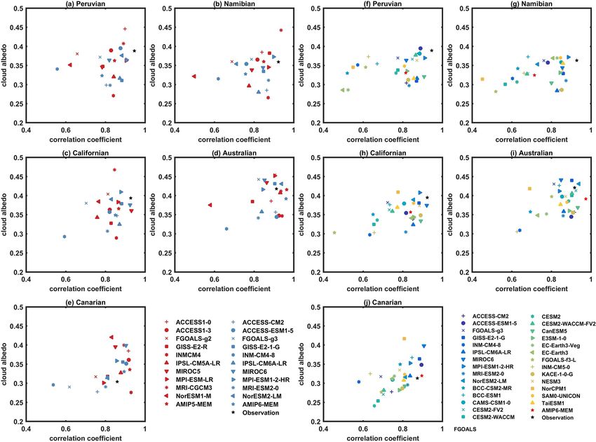
9812                                            B. Jian et al.: Evaluation of the CMIP6 cloud albedo and its controlling factors

Table 1. The list of CMIP5 models used in the study and their atmospheric horizontal resolutions.

            Model name            Origin                                                                      Resolution (lat × long)
       1    ACCESS1-0             Commonwealth Scientific and Industrial Research Organization and Bureau     145 × 192
                                  of Meteorology, Australia
       2    ACCESS1-3             Commonwealth Scientific and Industrial Research Organization and Bureau     145 × 192
                                  of Meteorology, Australia
       3    FGOALS-g2             Institute of Atmospheric Physics, Chinese Academy of Sciences and Ts-       60 × 128
                                  inghua University, China
       4    GISS-E2-R             NASA Goddard Institute for Space Studies, USA                               90 × 144
       5    INMCM4                Institute of Numerical Mathematics, Russia                                  120 × 180
       6    IPSL-CM5A-LR          Institut Pierre Simon Laplace, France                                       96 × 96
       7    MIROC5                AORI, NIES and JAMSTEC, Japan                                               128 × 256
       8    MPI-ESM-LR            Max Planck Institute for Meteorology, Germany                               96 × 192
       9    MRI-CGCM3             Meteorological Research Institute, Japan                                    160 × 320
       10   NorESM1-M             Norwegian Climate Centre, Norway                                            96 × 144

marine stratocumulus cloud albedo were evaluated based on                 The invariable αcloud and αclear should be applied for the
the mass concentrations of hydrophilic black carbon (BC),                 same cloud type and ocean region. In this light, as in the
hydrophilic organic carbon (OC), sulfate aerosol (SO4 ), sul-             works in Klein and Hartmann (1993), this study also ana-
fur dioxide (SO2 ), the smallest particles dust (DU; i.e., 0.1–           lyzed only five marine stratocumulus regions: Peruvian (10–
1 µm size) and sea salt (SS; 0.03–0.1 µm size) at the 910 hPa             20◦ S, 80–90◦ W; A1), Namibian (10–20◦ S, 0–10◦ E; A2),
level. The meteorological variables include the monthly ver-              Californian (20–30◦ N, 120–130◦ W; A3), Australian (25–
tical velocity at 900 and 700 hPa (omega900 and omega700),                35◦ S, 95–105◦ E; A4) and Canarian (15–25◦ N, 25–35◦ W;
surface pressure, relative humidity at 700 hPa (RH700), air               A5). Previous study (Engström et al., 2014) has also demon-
temperature, the eastward wind, the northward wind, and sur-              strated that there is a near-linear relationship between cloud
face skin temperature data. In addition, the estimated inver-             cover and planetary albedo in these regions. Figure 1 illus-
sion strength (EIS) and horizontal temperature advection at               trates the locations of the above stratocumulus regions and
the surface (SSTadv) factors were also calculated. Finally, all           the near-global distribution of combined planetary albedo
of these meteorological parameters were used to investigate               averaged from Aqua and Terra during the continuous pe-
the meteorological effects on the cloud albedo (the units for             riod from 2003 to 2014. Here, EIS is defined in Wood and
aerosol mass concentrations, relative humidity, vertical ve-              Bretherton (2006):
locity, EIS and SSTadv are kg m−3 , %, Pa s−1 , K and K s−1 ,                          850
respectively).                                                            EIS = LTS − 0m   (Z700 − ZLCL ) ,                             (3)

                                                                          where the lower-tropospheric stability (LTS) is defined as
2.4    Methods
                                                                          the difference in potential temperature between 700 hPa and
                                                                          the surface, 0m850 is the moist-adiabatic lapse rate at 850 hPa,
The planetary albedo (α) can be calculated mainly from the
cloud fraction f (Bender et al., 2011) as expressed in Eq. (1):           and Z700 and ZLCL are the height of the 700 hPa level and
                                                                          the lifting condensation level relative to the surface, respec-
α = αcloud f + αclear (1 − f ),                                  (1)      tively. As in Wood and Bretherton (2006), we assumed the
                                                                          surface relative humidity of 80 % to simplify the calculation
where αcloud and αclear denote the albedo under cloudy-sky                of surface dew point temperature. ZLCL was calculated based
and clear-sky conditions, respectively. For a given region                on the method of Georgakakos and Bras (1984). In addition,
where the cloud and surface type are homogeneous (i.e., con-              SSTadv was obtained by Eq. (4) as in Qu et al. (2015):
stant αcloud and αclear ), a change in α should be driven by a                            u    ∂SST v ∂SST
change in the cloud fraction f . The cloud albedo can be es-              SSTadv = −                       ,                            (4)
                                                                                       RE cos φ ∂λ RE ∂φ
timated by the derivative of Eq. (1) as in Eq. (2):
                                                                          where u and v represent the eastward and northward hor-
αcloud = dα/df + αclear .                                        (2)      izontal wind components at 1000 hPa, respectively, and φ

Atmos. Chem. Phys., 21, 9809–9828, 2021                                                     https://doi.org/10.5194/acp-21-9809-2021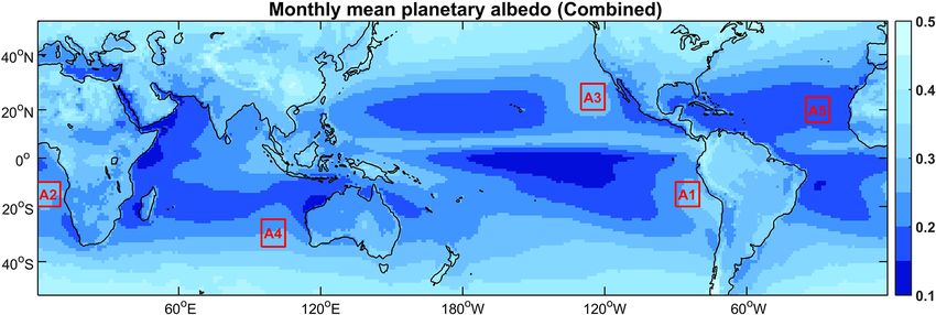
B. Jian et al.: Evaluation of the CMIP6 cloud albedo and its controlling factors                                                  9813

Table 2. The list of CMIP6 models used in the study and their atmospheric horizontal resolutions.

        Model name                 Origin                                                                     Resolution (lat × long)
  1     ACCESS-CM2                 Commonwealth Scientific and Industrial Research Organization and Bureau    145 × 192
                                   of Meteorology, Australia
  2     ACCESS-ESM1-5              Commonwealth Scientific and Industrial Research Organization and Bureau    145 × 192
                                   of Meteorology, Australia
  3     FGOALS-g3                  Institute of Atmospheric Physics, Chinese Academy of Sciences and Ts-      80 × 180
                                   inghua University, China
  4     GISS-E2-1-G                NASA Goddard Institute for Space Studies, USA                              90 × 144
  5     INM-CM4-8                  Institute for Numerical Mathematics, Russia                                120 × 180
  6     IPSL-CM6A-LR               Institut Pierre Simon Laplace, France                                      143 × 144
  7     MIROC6                     AORI, NIES and JAMSTEC, Japan                                              128 × 256
  8     MPI-ESM1-2-HR              Max Planck Institute for Meteorology, Germany                              192 × 384
  9     MRI-ESM2-0                 Meteorological Research Institute, Japan                                   160 × 320
  10    NorESM2-LM                 Norwegian Climate Centre, Norway                                           96 × 144
  11    BCC-CSM2-MR                Beijing Climate Center, China                                              160 × 320
  12    BCC-ESM1                   Beijing Climate Center, China                                              64 × 128
  13    CAMS-CSM1-0                Chinese Academy of Meteorological Sciences, China                          160 × 320
  14    CESM-FV2                   National Center for Atmospheric Research, Climate and Global Dynamics      96 × 144
                                   Laboratory, USA
  15    CESM2-WACCM                National Center for Atmospheric Research, Climate and Global Dynamics      192 × 288
                                   Laboratory, USA
  16    CESM2                      National Center for Atmospheric Research, Climate and Global Dynamics      192 × 288
                                   Laboratory, USA
  17    CESM2-WACCM-FV2            National Center for Atmospheric Research, Climate and Global Dynamics      96 × 144
                                   Laboratory, USA
  18    CanESM5                    Canadian Centre for Climate Modelling and Analysis, Environment and Cli-   64 × 128
                                   mate Change Canada, Canada
  19    E3SM-1-0                   LLNL, ANL, BNL, LANL, LBNL, ORNL, PNNL and SNL, USA                        180 × 360
  20    EC-Earth3-Veg              EC-Earth consortium (27 institutions in Europe)                            256 × 512
  21    EC-Earth3                  EC-Earth consortium (27 institutions in Europe)                            256 × 512
  22    FGOALS-f3-L                Chinese Academy of Sciences, China                                         180 × 288
  23    INM-CM5-0                  Institute for Numerical Mathematics, Russian Academy of Science, Russia    120 × 180
  24    KACE-1-0-G                 National Institute of Meteorological Sciences and Korea Meteorological     144 × 192
                                   Administration, Republic of Korea
  25    NESM3                      Nanjing University of Information Science and Technology, China            96 × 192
  26    NorCPM1                    NorESM climate modeling consortium consisting of CICERO, MET-              96 × 144
                                   Norway, NERSC, NILU), UIB, UIO and UNI, Norway
  27    SAM0-UNICON                Seoul National University, Republic of Korea                               192 × 288
  28    TaiESM1                    Research Center for Environmental Changes, Academia Sinica, Taiwan         192 × 288

https://doi.org/10.5194/acp-21-9809-2021                                                  Atmos. Chem. Phys., 21, 9809–9828, 2021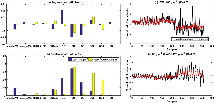
9814 B. Jian et al.: Evaluation of the CMIP6 cloud albedo and its controlling factors
and λ are latitude and longitude, respectively. RE is the 3 Results
mean Earth radius, and SST is the surface skin tempera-
ture. A positive/negative SSTadv indicates warm/cold advec- 3.1 Satellite observations and CMIP5/6 simulations
tion. The SSTadv can affect the moisture transport within the
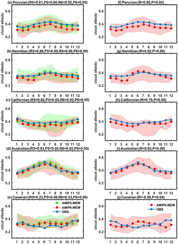
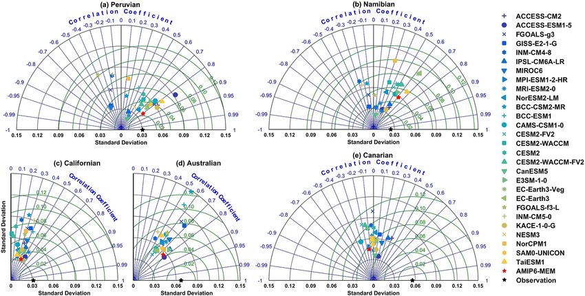
cloud layer by influencing the surface sensible and latent heat The first two columns in Fig. 2 (from panels a to e) show
fluxes and, consequently, influence the thickness of marine the estimated long-term mean cloud albedo corresponding
stratocumulus clouds (George and Wood, 2010). to the correlation between planetary albedo and cloud frac-
In the study, to avoid influence from a seasonal cycle, the tion over the five regions from the observations and 22
long-term mean analyses are implemented with deseasonal- AMIP5 and AMIP6 models, including 10 individual mod-
ized monthly mean data processed by removing a mean sea- els and an ensemble mean for AMIP5 and AMIP6 (repre-
sonal cycle and then adding the monthly mean value to the sented by AMIP5-MEM and AMIP6-MEM), during the pe-
interannual anomaly data. The selection of variables is a cru- riod from 2003 to 2008. For the combined satellite obser-
cial step to build a multiple linear regression model of the vations, the correlation coefficient values are above 0.85 in
monthly cloud albedo as a function of meteorological fac- all regions. The correlation over the Peruvian region was the
tors and aerosol types under two different LWP scenarios largest (∼ 0.95), while a relatively weak correlation (∼ 0.88)
(LWP < 65 g m−2 and 65 g m−2 < LWP < 120 g m−2 ). This appeared in the Canarian region. Such a high correlation be-
study selected suitable variables based on correlation anal- tween planetary albedo and cloud fraction further indicates
ysis. If the correlation between the cloud albedo and a can- the homogeneity of cloud and surface types over these re-
didate is significant at a 90 % confidence level, the variable gions. The regressed cloud albedo from the satellite ranged
was considered as a predictor factor. Furthermore, the partial from 0.30 to 0.42 for the five stratocumulus regions, which
least squares were used to reduce the collinearity between is consistent with previous studies (Bender et al., 2011; En-
the selected variables (McCoy et al., 2017). The regression gström et al., 2014). As the values averaged over Aqua and
model of cloud albedo αcloud is as follows: Terra albedos and cloud fractions were used as the observa-
I J tions in this study, the regressed cloud albedo values need to
X X
αcloud = ai Mi + bj log10 Aj + c, (5) be within the range of the Aqua and Terra values (Engström
i=1 j =1 et al., 2014). Regarding the AMIP5 and AMIP6 models, a
higher correlation (> 0.8) appeared for most models in the
where a and b are regression coefficients, c is a constant five regions, especially higher in the Australian and Canarian
term, Mi represents the ith meteorological predictor, I is the regions. In the Peruvian, Namibian and Californian regions,
number of meteorological predictor variables, Aj is the j th the correlations of the observations were relatively higher
aerosols predictor, and J is the number of aerosol predictor than those of most climate models, while the observed corre-
variables. lation was approximately close to the median value of model
The relative contributions of each predictor to the change simulations in the Australian and Canarian regions.
in the cloud albedo (Huang and Yi, 1991) were evaluated Although previous studies indicated that some CMIP6
using Eq. (6): models updated the cloud physical parameterization in the
new version (Seland et al., 2020; Kawai et al., 2019), the
" !#
m a
1X 2
X 2
Rj = T Tij , (6) correlation coefficients of the AMIP6 models between plan-
m i=1 ij j =1 etary albedo and cloud fraction showed a lower value than
where m is the number of the monthly samples, a is the num- those of the AMIP5, indicating that the linear relationship
ber of predictors, and Tij is the product of the regression co- between cloud fraction and planetary albedo in the AMIP6
efficients of each term (bj ) and predictor variables (xij ). models’ simulations is not superior to that of AMIP5. While
After removing the effect of meteorological factors, we the AMIP6 simulations displayed a similar spread in the
further investigated the pure relationship between aerosols estimated cloud albedo for all regions, some AMIP6 mod-
and the cloud albedo using the partial correlations between els produced a lower correlation coefficient than those of
αcloud and log10 A, as expressed in Eq. (7): the AMIP5 models (e.g., AMIP6/INM-CM4-8). Notably, the
AMIP5-MEM and AMIP6-MEM always produced a worse
rα ·log A − rαcloud ·M rlog10 A·M correlation relationship and more irrational cloud albedo val-
rαcloud log10 A·M = qcloud 10 q , (7)
1 − rα2cloud ·M 1 − rlog
2 ues, indicating that the AMIP5 and AMIP6 models have a
A·M 10
lack of skill in simulating cloud properties over the marine
where rαcloud ·log10 A , rαcloud ·M and rlog10 A·M are the total cor- stratocumulus regions.
relation between each variable pair, and rαcloud log10 A·M is the The third and fourth columns in Fig. 2 (from panel f to
correlation between αcloud and log10 A which eliminates the j) also show the estimated long-term mean cloud albedo and
effects of meteorological factors M. More details on the par- the correlation between planetary albedo and cloud fraction
tial correlation are described in Jiang et al. (2018) and En- over the five regions for the observations and 29 AMIP6
gström and Ekman (2010). models from 2003 to 2014. The simulated correlation exhib-
Atmos. Chem. Phys., 21, 9809–9828, 2021 https://doi.org/10.5194/acp-21-9809-2021B. Jian et al.: Evaluation of the CMIP6 cloud albedo and its controlling factors 9815 Figure 1. Near-global distribution of combined planetary albedo averaged from Aqua and Terra during 2003–2014. Red rectangular boxes indicate the five regions used chosen for the analysis: (A1) Peruvian, (A2) Namibian (A3) Californian, (A4) Australian and (A5) Canarian. Figure 2. The estimated long-term mean cloud albedo and corresponding correlation coefficient from the relation between planetary albedo and cloud fraction (a–e) from satellite observations (black symbol), 11 AMIP5 (red symbols) models and 11 AMIP6 (blue symbols) models during 2003–2008 and (f–j) from satellite observations and 29 AMIP6 models during 2003–2014 over the (a, f) Peruvian, (b, g) Namibian (c, h) Californian, (d, i) Australian and (e, j) Canarian regions. https://doi.org/10.5194/acp-21-9809-2021 Atmos. Chem. Phys., 21, 9809–9828, 2021
9816 B. Jian et al.: Evaluation of the CMIP6 cloud albedo and its controlling factors
ited a larger spread in the Peruvian and Namibian regions Compared with AMIP5-MEM, the regressed monthly
than those in other regions, indicating that the AMIP6 mod- cloud albedo of AMIP6-MEM showed a better correla-
els have a lack of capacity to capture the linear relationship tion with the satellite-regressed values. However, the per-
between planetary albedo and cloud fraction. The cloud albe- formance of AMIP5-MEM in reproducing monthly cloud
dos were underestimated in most CMIP6/AMIP models com- albedo and its amplitude (the difference between the maxi-
pared with the satellite-based cloud albedos. The Australian mum and minimum values of cloud albedo) was better than
(0.30–0.43) and Canarian (0.24–0.42) regions displayed a that of AMIP6-MEM. Furthermore, the monthly cloud albe-
larger intermodel variability in the cloud albedo than other dos obtained from the satellite and models displayed an ob-
regions due to a poor skill in simulating the cloud properties vious seasonal cycle in all regions except for the Canarian re-
(e.g., LWP and COT). Over the Canarian regions, the correla- gion. This may be related to the fact that a weaker linear rela-
tion and cloud albedo of AMIP6-MEM showed good agree- tionship between monthly cloud cover and planetary albedo
ment with those of the satellite observations compared with may exist in the Canarian region, resulting in a significant
those of the individual AMIP6 models, resulting from the change in the estimated cloud albedo (see Fig. S2).
offsetting effect between models. Overall, the AMIP6 mod- In addition, the monthly cloud albedo time series for the
els reproduced the cloud albedo and correlation well in the satellite and AMIP6-MEM for the period from 2003 to 2014
Australian region while having a higher uncertainty in the in the five regions are also shown in Fig. 3f–j, which are con-
model’s simulations, i.e., a larger intermodal spread, in the sistent with Fig. 3a–e, indicating that the simulation capa-
Peruvian region (Engström et al., 2014). bility of the AMIP6-MEM in different regions does not im-
Engström et al. (2014) also found that CMIP5 models sim- prove significantly with the expansion of the simulation time
ulating a higher cloud cover have a tendency to produce a and the increase in the model numbers. The amplitudes of
smaller cloud albedo value. Darker clouds can offset the con- the cloud albedo simulated from the model were larger than
tribution of the higher cloud cover to the planetary albedo, those of the satellite in the Peruvian, Namibian and Califor-
resulting in a relatively consistent model-driven planetary nian regions and smaller in the Australian and Canarian re-
albedo. This is a presentation of the “too few, too bright” gions. Note that in the Australian region, the monthly cloud
problem that persists in general circulation models (GCMs; albedo exhibited a larger variation than that in other regions
Nam et al., 2012). To validate whether or not this problem based on the satellite-based observations, which means that
has been improved in the AMIP6 models, we compared the the cloud optical properties (e.g., COT and cloud effective ra-
relationship between regressed cloud albedo and cloud frac- dius) have been considerably changed within the Australian
tion (See Fig. S1 in the Supplement). The correlations driven region.
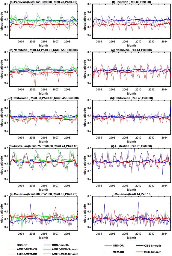
by the 28 AMIP6 models were −0.28, 0.19, −0.11, −0.71 This study further assessed the performance of the AMIP6
and 0.43 for the Peruvian, Namibian, Californian, Australian models in reproducing the cloud albedo time series. Fig-
and Canarian regions, respectively. Compared with the re- ure 4a–e provide the Taylor diagrams (Taylor, 2001) for
sults from the CMIP5 models (Engström et al., 2014), notice- the five regions, which include the correlation coefficients,
able progress was found in the Namibian and Californian re- the centered root mean square error (RMSE, the green cir-
gions, while a high negative correlation was simulated in the cle), and the standard deviation value between individual
Australian region, indicating that the new generation mod- AMIP6 models and the satellite-based observations. The cen-
els need to be further improved to resolve the long-standing tered RMSE and the standard deviation values represent the
problem. model’s ability to reproduce the phase and amplitude of the
The monthly cloud albedo time series regressed from the variable, respectively. Correlation coefficients greatly varied
satellite, MEM and AMIP6-MEM for the 6-year period from by region, ranging from negative (Peruvian, Namibian and
2003 to 2008 over the five regions are shown in Fig. 3a– Canarian) to positive values. Compared with other regions,
e. The temporal correlations (R5/R6) and correspond- most of the models showed a high positive correlation (> 0.6)
ing confidence value (P5/P6) between simulated (AMIP5- in the Peruvian region. The model-driven cloud albedo was
MEM/AMIP6-MEM) and satellite-regressed monthly cloud most poorly correlated with the observations in the Canarian
albedo time series are also given in Fig. 3a–e. Note that the region, e.g., < 0.4 or negative values. In contrast, in the Aus-
smoothed time series were produced by 12-month smooth- tralian region, all models showed a significant positive corre-
ing. The statistical results showed that the R5/R6 val- lation (> 0.4). The standard deviation values of the models in
ues were 0.62/0.78, 0.44/0.55, 0.38/0.45, 0.75/0.74 and the Peruvian, Namibian and Californian regions were in the
0.00/0.05 for the Peruvian, Namibian, Californian, Aus- range of 0.02–0.09, 0.02–0.11 and 0.03–0.10, respectively,
tralian and Canarian regions, respectively. Among them, the and 0.03 for the satellite-based observations. This result in-
correlations only in the Canarian region were insignificant dicates that most of the models overestimate the amplitude of
(i.e., P5/P6 = 1.00/0.70). A high positive correlation ap- the cloud albedo time series in the regions. Some models pro-
peared in the Australian region (> 0.70), indicating that the duced the standard deviation values of cloud albedos 3 times
changes in the cloud albedo are well captured by the models. larger than the observations. It is evident that the standard de-
viation values of the simulated cloud albedo in the Australian
Atmos. Chem. Phys., 21, 9809–9828, 2021 https://doi.org/10.5194/acp-21-9809-2021B. Jian et al.: Evaluation of the CMIP6 cloud albedo and its controlling factors 9817 Figure 3. Monthly mean time series of estimated cloud albedo (a–e) from AMIP5 and AMIP6 multimodel ensemble mean during 2003– 2008 and (f–j) from AMIP6 multimodel ensemble mean during 2003–2014 compared with satellite observations over the (a, f) Peruvian, (b, g) Namibian, (c, h) Californian, (d, i) Australian and (e, j) Canarian regions. https://doi.org/10.5194/acp-21-9809-2021 Atmos. Chem. Phys., 21, 9809–9828, 2021
9818                                         B. Jian et al.: Evaluation of the CMIP6 cloud albedo and its controlling factors

region were closer to the observed value than that of other         ist in the boundary layer at the earlier time of the biomass
regions, indicating that the AMIP6 models also perform well         burning seasons and are mainly located above the clouds in
in simulating the amplitude of the monthly cloud albedo time        September to October, which is caused by the northwest-
series in this region. Overall, the intermodal variability in the   ward transportation of the biomass burning aerosols from the
correlation coefficient, RMSE and standard deviation values         African continent. However, Fig. 5b shows that the peak of
was the smallest in the Australian region, while the largest        the cloud albedo occurred in July and then continuously de-
was in the Peruvian region.                                         creased from August to October in the Namibian region, in-
   Further, Fig. 5 shows the annual cycles of the cloud albedo      dicating that it is difficult to explain the changes in the cloud
estimated by the satellite and AMIP5 and AMIP6 models for           albedo by the negative semi-direct effect of the biomass
the five regions. The seasonal variation in the cloud albedo        burning aerosols. This result is consistent with the work of
in each region takes a shape of a single peak distribution.         Bender et al. (2016) which concluded that the direct effect
In terms of similarity among regions, the cloud albedo in all       and positive semi-direct effect are the main aerosol effects
regions reached the maximum value during the boreal win-            (Wilcox, 2012). That is, clouds become darker under a pol-
ter season, i.e., December to January in the Northern Hemi-         luted environment. Regarding the seasonal cycles of cloud
sphere and June to July in the Southern Hemisphere. Many            droplet number concentration, Nd , we found that the sea-
previous studies have demonstrated that the seasonal varia-         sonal cycles of the cloud albedo in the Namibian region were
tions in marine cloud properties (e.g., cloud fraction, LWP         highly correlated with those of Nd obtained from the Cloud-
and cloud thickness) are strongly affected by meteorologi-          Aerosol Lidar and Infrared Pathfinder Satellite Observations
cal conditions (Lin et al., 2009; Wood, 2012; Dong et al.,          (CALIPSO) (Li et al., 2018), whereas the seasonal cycles of
2014). Employing a 19-month record of ground-based li-              Nd and the cloud albedo showed opposite seasonal changes
dar and radar observations from the Atmospheric Radiation           to each other in the California region. The relationship be-
Measurement Program Azores site, for example, Dong et               tween the Nd and the cloud albedo varies with different re-
al. (2014) found that the seasonal variations in cloud thick-       gions, which may be caused by the effect of meteorologi-
ness and LWP are closely related to the seasonal synoptic           cal conditions. These results indicate that it is a challenge to
patterns (e.g., transport of water vapor, relative humidity,        study the variability in the cloud albedo over the marine stra-
high and low pressure system). Furthermore, the influence of        tocumulus regions under various meteorological and aerosol
aerosol loading is non-neglectable. While the aerosols act as       conditions.
CCN, the concentration of CCN can significantly influence              Figure 5a–e show the seasonal cycles of cloud albedo
the cloud albedo of low clouds (Twomey, 1974). On the other         in the five regions during a period from 2003 to 2008 for
hand, absorbing aerosols near stratocumulus may enhance             the AMIP5 and AMIP6 and the satellite-based observations.
absorbing solar energy, resulting in an influence on the dy-        Shaded areas in Fig. 5 represent the range of the cloud albedo
namical evolution of stratocumulus causing a change in the          simulated by the 22 models. The R5/R6 and P5/P6 val-
cloud albedo (Wilcox, 2010). The seasonal cycle of the cloud        ues for the seasonal cycles of the cloud albedo obtained
albedo in the Australian region showed the largest amplitude        from the models and the satellite-based observations are
among the five regions (ranging from 0.37 to 0.52), while           also given in Fig. 5. For the AMIP5-MEM and AMIP6-
the amplitudes in other regions were less than 0.10. Such a         MEM, the correlations of the cloud albedo seasonal cycles
result means that the meteorological conditions and aerosol         between the models and the observations are highly posi-
loadings of the cloud system in the Australian region have          tive in all regions (R5/R6 > 0.6), except for the Canarian re-
a relatively larger seasonal variation compared with those in       gion (R5/R6 = 0.22/0.53). The R values were the largest in
other regions.                                                      the Namibian (R5/R6 = 0.82/0.92) and Australian regions
   The COT usually increases with an increase in cloud LWP,         (R5/R6 = 0.93/0.92). Overall, the results of AMIP6 were
resulting in an increase in the cloud albedo (Wood, 2012).          slightly superior to those of AMIP5, especially in the Ca-
Gryspeerdt et al. (2019) also concluded that LWP is the main        narian region. However, the seasonal cycles of cloud albedo
factor controlling liquid cloud albedo. Thus, this study in-        estimated from the AMIP6-MEM in the Canarian region for
vestigated the seasonal variation of LWP and found that the         12 years from 2003 to 2014 (Fig. 5j) exhibited a significant
change in LWP is strongly correlated with the change in             negative correlation with that of the satellite-based observa-
cloud albedo in the Peruvian, Australian and Canarian re-           tions, indicating AMIP6-MEM still has a lack of skill in cap-
gions (see Fig. S3). For the Namibian region, however, many         turing the seasonal cycle of the cloud albedo in this region
studies have shown that the continuous transportation of ab-        even if the numbers of AMIP6 models increases.
sorbing biomass burning aerosols from Africa to the region
during the African biomass burning season from August to            3.2   The impacts of different aerosol types and
October (Das et al., 2017) can reside above the clouds, re-               meteorological factors on cloud albedo changes
sulting in an increase in the cloud albedo by thickening the
stratocumulus (Wilcox, 2010, 2012). Zuidema et al. (2018)           Cloud liquid water may affect the COT, which is subse-
also found that the biomass burning aerosols generally ex-          quently influencing the cloud albedo (Wood, 2012). Further-

Atmos. Chem. Phys., 21, 9809–9828, 2021                                               https://doi.org/10.5194/acp-21-9809-2021
B. Jian et al.: Evaluation of the CMIP6 cloud albedo and its controlling factors                                                     9819

Figure 4. Taylor diagrams for monthly estimated cloud albedo between individual AMIP6 models and satellite observations during 2003–
2014 over the (a) Peruvian, (b) Namibian, (c) Californian, (d) Australian and (e) Canarian regions. The green circles indicate the centered
root mean square error.

more, the change in LWP also may influence the relation-                creases with increasing BC/SO2 /SS and decreases with in-
ship between aerosols and cloud properties (Roberts et al.,             creasing DU/OC. Figure 6b also clearly shows that DU, BC
2008; Gryspeerdt et al., 2019; Douglas and L’Ecuyer, 2019).             and OC make a larger contribution to the change in the cloud
For example, the effect of aerosols on the cloud albedo may             albedo compared with other predictors, e.g., omega900, EIS
be weakened by a change in the LWP (Han et al., 2002;                   and RH700. Under LWP > 65 g m−2 , the contribution of DU
Twohy, 2005). Based on in situ observations, recent stud-               to the cloud albedo was the largest. In addition, SO2 and SO4
ies found that the relationship between aerosol concentra-              also considerably contributed to the cloud albedo.
tion and cloud droplet effective radius changes from nega-                 In addition to the effects of LWP, the difference in the
tive to positive when liquid water content increases (Qiu et            relative contribution may be induced by the regional vari-
al., 2017; Zhao et al., 2019b). Considering the effect of LWP,          ability in aerosol types. A smaller LWP mainly appeared in
this study evaluated the impact of meteorological parame-               the Namibian and Canarian regions where the main aerosol
ters and aerosol types on the cloud albedo at different LWP             types are DU and BC, while lower BC loadings were found
ranges in order to evaluate the influence of LWP on cloud               in the regions with a larger LWP (Fig. S4). While the posi-
albedo. Firstly, the 720 monthly sample data points obtained            tive coefficient for BC reflects the indirect effect of aerosols
from the five regions were divided into two groups based on             on the cloud albedo, the negative dependency of BC may rep-
the range of monthly mean LWP values: LWP ≤ 65 g m−2                    resent the direct and semi-direct effects of absorbing aerosols
and 65 g m−2 < LWP ≤ 120 g m−2 . Here, the threshold of                 (Johnson et al., 2004; Bender et al., 2016). For example,
65 g m−2 for LWP was chosen to evenly split the samples.                Johnson et al. (2004) found that absorbing aerosols in clouds
   Figure 6a–b show the regression coefficients in the par-             can make the clouds warmer and thinner, resulting in a de-
tial correlation calculation and the relative contributions for         crease in cloud albedo. Moreover, McCoy et al. (2018) found
individual variables related to cloud albedo changes under              a negative dependence of Nd on BC in regions with low BC
different LWP conditions. Normalized variables were incor-              loadings. This means that a decrease in the cloud albedo may
porated into the regression models. There is a considerable             be associated with a decrease in Nd . The dependence of Nd
discrepancy in the results between the two groups. For the              on OC has also been investigated in previous studies (McCoy
lower LWP bin (i.e., LWP ≤ 65 g m−2 ), the results showed               et al., 2018; Li et al., 2018), and a negative dependence of Nd
that the regression coefficient of BC/SO2 /SS to the cloud              on OC has been found in some marine regions. The negative
albedo was positive, while DU- and OC-related coefficients              sensitivities of OC to the cloud albedo may be attributed to a
were negative, which indicates that the cloud albedo in-                decrease in Nd with an increase in OC.

https://doi.org/10.5194/acp-21-9809-2021                                                  Atmos. Chem. Phys., 21, 9809–9828, 2021
9820                                           B. Jian et al.: Evaluation of the CMIP6 cloud albedo and its controlling factors

Figure 5. Annual cycles of the cloud albedo estimated by (a–e) AMIP5 and AMIP6 multimodel ensemble mean during 2003–2008 and
(f–j) AMIP6 multimodel ensemble mean during 2003–2014 compared with satellite observations over the (a, f) Peruvian, (b, g) Namibian,
(c, h) Californian, (d, i) Australian and (e, j) Canarian regions. The green and red shaded areas indicate the range of the cloud albedo
simulated by AMIP5 and AMIP6 models, respectively. The temporal correlations (R5/R6/R value) and P5/P6/P value (if P5/P6/P < 0.10,
indicating the correlation R5/R6/R is significant) for the seasonal cycles of the cloud albedo obtained from satellite-based observations and
models are given in parentheses.

   Dust is a crucial predictor of the cloud albedo, and the co-          Nd by consuming the supersaturation of clouds. However,
efficient of DU was negative for the two datasets divided in             McCoy et al. (2017) estimated the indirect effect of aerosol
this study, which may be induced by the semi-direct effects              from satellite observations and reanalysis data and found that
of absorbing aerosols. In the literature, many studies have              the dust has a limited impact on Nd in different stratocumu-
examined the impacts of dust aerosols on stratocumulus (Do-              lus regions. Pradelle et al. (2002) employing satellite obser-
herty and Evan, 2014; Amiri-Farahani et al., 2017). For ex-              vations also investigated the effect of Saharan dust on marine
ample, Karydis et al. (2011) showed that aged dust reduces               stratocumulus clouds and found that minimum cloud albedo

Atmos. Chem. Phys., 21, 9809–9828, 2021                                                     https://doi.org/10.5194/acp-21-9809-2021
B. Jian et al.: Evaluation of the CMIP6 cloud albedo and its controlling factors                                                  9821

Figure 6. The (a) regression coefficients and corresponding (b) relative contribution of each predictor variable related to cloud albedo
from the multilinear regression models under two LWP conditions: LWP ≤ 65 g m−2 (blue) and 65 g m−2 < LWP ≤ 120 g m−2 (yellow).
Note that for ease of comparison, 11 variables are given in the figure, and variables without values are not predictive variables of
the sample group. The satellite- and model-driven normalized cloud albedo trained in two sample groups: (c) LWP ≤ 65 g m−2 and
(d) 65 g m−2 < LWP ≤ 120 g m−2 . The correlations (R value) between satellite- and model-driven normalized cloud albedo are given in
parentheses.

values appeared in regions with the most dust particles. They         tween the cloud albedo and near-surface wind speed, which
also found that the dust in a stratiform cloud may decrease           may explain the limited effect of SS on the cloud albedo.
the initial CCN and increase the effective droplet radius,               The coefficients of SO2 were positive for both datasets. In
which causes a reduction in the cloud albedo (Pradelle and            addition, the Twomey effect for SO2 was further pronounced
Cautenet, 2002). In addition, a recent study also showed that         under the condition with higher LWP. The previous studies
the dust aerosol can even further influence the meteorologi-          (e.g., McCoy et al., 2017; Li et al., 2018) showed that SO4
cal environment that the clouds form by both suppressing the          plays a key role in modulating Nd . Although their results
SST and affecting the temperature and humidity profile (Sun           showed significant positive coefficients of SO4 with Nd , this
and Zhao, 2020). A significant influence of dust on the cloud         study found an unexpected negative correlation of SO4 with
albedo in this study may be driven by the collected samples           the cloud albedo. Such a result may be driven by the fact that
in the five regions where the cloud albedo and dust highly            the sulfate aerosol particles and dust are externally mixed.
vary with the regions.                                                The previous studies showed that sulfate-covered dust can
   Under LWP ≤ 65 g m−2 , the coefficient of SS was a small           act as CCN, which may induce a decrease in the cloud albedo
positive value, while the correlation coefficient of sea salt         by enhancing the collision–coalescence progress of droplets
was insignificant under LWP > 65 g m−2 , which means that             (Levin et al., 1996; Rosenfeld et al., 2001).
these variables are not suitable as a predictor for estimat-             The results of this study showed a weak dependency of
ing the cloud albedo. This is consistent with the results of          the cloud albedo with omega900, RH700 and EIS. Under
McCoy et al. (2017, 2018) which indicate that the Nd is               LWP ≤ 65 g m−2 , the upward vertical velocity and RH700
weakly dependent on the SS, although sea salt is an effec-            have an unexpected negative but weak effect on the cloud
tive CCN. McCoy et al. (2018) have also validated the influ-          albedo, and the relative contributions of omega900 and
ence of SS on Nd with up-to-date observations. As submicron           RH700 are negligible. Under LWP > 65 g m−2 , no signif-
SS in the MERRA-2 reanalysis data can be simply predicted             icant correlation between the cloud albedo and omega900
from wind speed and SST by a parameterization (Jaeglé et              was found. Note that the analysis of this study employed the
al., 2011; McCoy et al., 2018; Li et al., 2018), the effect of SS     average data at the monthly scale rather than raw satellite
on the cloud albedo may be dependent on the relationship be-          measurements at an instantaneous scale, which may make
                                                                      the cloud albedo less sensitive to omega900. The coefficient

https://doi.org/10.5194/acp-21-9809-2021                                                Atmos. Chem. Phys., 21, 9809–9828, 2021
9822 B. Jian et al.: Evaluation of the CMIP6 cloud albedo and its controlling factors of RH700 was positive, and the relative contribution was In addition, to verify the sensitivity of the results to in- about 4 %. Generally, drier free-troposphere humidity usu- put data, we employ different datasets to perform the mul- ally drives stronger entrainment of dry air, which induces tilinear regression. The monthly Multisensor Advanced Cli- evaporating and raising lifted condensation level, resulting in matology of Liquid Water Path (MAC-LWP) is used to test a reduced cloud thickness (Wood, 2012; Eastman and Wood, the sensitivity of the results to the input LWP data (Elsaesser 2018). The positive dependency of the cloud albedo on EIS et al., 2017). Considering the differences in retrieval meth- was identified for the two datasets divided in this study, ods and values of the MODIS LWP and MAC-LWP datasets which may be caused by stronger inversions linked to in- (Greenwald, 2009), we used the threshold of 55 g m−2 for creased stability and reduced vertical exchange at cloud top, MAC-LWP to better split the samples evenly. The regressed resulting in thicker low clouds by keeping moisture trapped results are given in Fig. S5. We can see that the results did not in the marine boundary layer (MBL) (Scott et al., 2020). change significantly, indicating that the regressed results are Compared to other meteorological factors, the contribution relatively robust. For the reanalyzed dataset, ERA-5 reanal- of SSTadv to cloud albedo was larger and non-negligible ysis is considered to be the most state-of-the-art reanalysis in both datasets (7 %–9 %). Under LWP ≤ 65 g m−2 , the with higher temporal and spatial resolutions (Hersbach et al., SSTadv showed a negative coefficient. The cold advection 2019). We also used the ERA-5 data to perform the multiple usually thickens clouds by reducing low-level stability and regression model (see Fig. S6). Although the results change transporting more moisture into the MBL (George and Wood, slightly, the changed results do not affect the main conclu- 2010; Scott et al., 2020). Under LWP > 65 g m−2 , the coeffi- sions. cient of SSTadv was positive, which is hard to be explained It is also found from Fig. 6 that changes in LWP can also by the aforementioned mechanism. By analyzing the corre- cause an alteration of the relationship between aerosol and lation between LWP and SSTadv, we found that there was the cloud albedo. To further investigate the influence of me- no significant correlation between them. This indicates that teorological factors on the relationship, the partial correla- the surface temperature advection may affect cloud albedo tions were calculated to eliminate the influence of meteoro- in other ways than by affecting the moisture in cloud layers. logical parameters individually or simultaneously. If the par- Furthermore, dust can affect the meteorological environment tial correlation is similar to the total correlation, it means through radiative effects; consequently, the positive coeffi- that the influence of meteorological factors on the relation- cient found in this study may be a reflection of their effects ship is limited. In contrast, the influence of meteorological (Sun and Zhao, 2020; Huang et al., 2021). The coefficients of factors on the relationship may be significant if the partial the omega700 were negative for both datasets. The downdraft correlation and the total correlation are the opposite sign. allowed dry air above the cloud to enter the clouds, causing Given six meteorological parameters (omega700, omega900, evaporation and making cloud droplets smaller and fewer, re- RH700, EIS, SSTadv and LWP) considered in this study, the sulting in reducing the cloud albedo (Yang et al., 2019). Note total correlation and partial correlation between the cloud that the role of omega700 was very weak under the condition albedo and different aerosols for two sample groups are given with higher LWP, and its contribution was negligible. in Table 3. Under LWP ≤ 65 g m−2 , the correlations of all The analysis of the relative contribution of each predic- aerosol types were weakened when eliminating the effects tor variable was similar to the results of the coefficients. of meteorological factors. When the influence of EIS and Under LWP ≤ 65 g m−2 , DU and BC contributed approxi- LWP were eliminated, the correlation of DU becomes much mately 63 % of the variations of the cloud albedo in the weaker, indicating that the correlation of DU is sensitive regression model. Note that the contribution of omega700 to EIS and LWP. On the contrary, the correlations of BC, and SSTadv was non-negligible, accounting for 18 %. Un- OC and SO4 were stronger when the influence of LWP was der LWP > 65 g m−2 , the contribution of DU and SO2 to the eliminated. In addition, most aerosol types were sensitive to change in cloud albedo was about 61 %. DU has the largest SSTadv except for the SS. The correlation of BC/OC ranged relative contribution to the cloud albedo changes (∼ 35 %) in from 0.21/0.20 to −0.03/−0.05 by eliminating the influence both datasets. of SSTadv, indicating that the relationship between BC/OC The normalized satellite-based and model-driven cloud and the cloud albedo is extremely sensitive to the influences albedos under different cloud water conditions are shown of SSTadv. Under LWP > 65 g m−2 , the correlations of all in Fig. 6c–d, in which the correlation (R) between the two aerosol types varied significantly by eliminating the influ- cloud albedos is given in parentheses. A larger R value indi- ence of all meteorological parameters. For example, the cor- cates a better model. Both of the correlation coefficients are relation of BC/DU/OC ranged from −0.47/−0.49/−0.45 to greater than 0.65, indicating the regression model properly −0.01/ − 0.02/ − 0.03. This indicates that the cloud–aerosol captures the changes in the cloud albedo for the two datasets. interaction is more sensitive to the response of meteorologi- A considerable part of the variation in cloud albedo can be cal conditions at higher LWP conditions. Although the con- explained by the change in meteorological parameters and tribution of meteorological parameters to the change in the mass concentrations of different aerosol types. cloud albedo is only a small part based on the relative con- Atmos. Chem. Phys., 21, 9809–9828, 2021 https://doi.org/10.5194/acp-21-9809-2021
You can also read