Destruction and reinstatement of coastal hypoxia in the South China Sea off the Pearl River estuary
←
→
Page content transcription
If your browser does not render page correctly, please read the page content below
Biogeosciences, 18, 2755–2775, 2021
https://doi.org/10.5194/bg-18-2755-2021
© Author(s) 2021. This work is distributed under
the Creative Commons Attribution 4.0 License.

Destruction and reinstatement of coastal hypoxia in the
South China Sea off the Pearl River estuary
Yangyang Zhao1,2 , Khanittha Uthaipan1 , Zhongming Lu3 , Yan Li1 , Jing Liu1 , Hongbin Liu4,5 , Jianping Gan3,5,6 ,
Feifei Meng1 , and Minhan Dai1
1 StateKey Laboratory of Marine Environmental Science, College of Ocean and Earth Sciences,
Xiamen University, Xiamen, 361102, China
2 Environmental Physics, Institute of Biogeochemistry and Pollutant Dynamics, ETH Zurich, 8092 Zurich, Switzerland
3 Division of Environment and Sustainability, The Hong Kong University of Science and Technology,

Kowloon, Hong Kong SAR, China
4 Division of Life Science, The Hong Kong University of Science and Technology, Kowloon, Hong Kong SAR, China
5 Department of Ocean Science, The Hong Kong University of Science and Technology, Kowloon, Hong Kong SAR, China
6 Department of Mathematics, The Hong Kong University of Science and Technology, Kowloon, Hong Kong SAR, China

Correspondence: Minhan Dai (mdai@xmu.edu.cn)

Received: 22 September 2020 – Discussion started: 12 October 2020
Revised: 17 March 2021 – Accepted: 17 March 2021 – Published: 30 April 2021

Abstract. We examined the evolution of intermittent hypoxia      1   Introduction
off the Pearl River estuary based on three cruise legs con-
ducted in July 2018: one during severe hypoxic conditions
before the passage of a typhoon and two post-typhoon legs        Coastal hypoxia has been increasingly exacerbated near the
showing destruction of the hypoxia and its reinstatement. The    mouths of large rivers as a consequence of anthropogenic nu-
lowest ever recorded regional dissolved oxygen (DO) con-         trient inputs (Gilbert et al., 2010; Rabalais et al., 2014; Breit-
centration of 3.5 µmol kg−1 (∼ 0.1 mg L−1 ) was observed in      burg et al., 2018). The rise in the size, intensity and frequency
bottom waters during leg 1, with an ∼ 660 km2 area expe-         of eutrophication-induced hypoxia exposes coastal oceans to
riencing hypoxic conditions (DO < 63 µmol kg−1 ). Hypoxia        a higher risk of elevated N2 O and CH4 production; enhanced
was completely destroyed by the typhoon passage but was          ocean acidification; and associated reductions in biodiversity,
quickly restored ∼ 6 d later, resulting primarily from high      shifts in community structures, and negative impacts on food
biochemical oxygen consumption in bottom waters that av-         security and livelihoods (Diaz and Rosenberg, 2008; Vaquer-
eraged 14.6 ± 4.8 µmol O2 kg−1 d−1 . The shoreward intru-        Sunyer and Duarte, 2008; Naqvi et al., 2010).
sion of offshore subsurface waters contributed to an addi-          Coastal hypoxia can be intermittent due to the dynamic
tional 8.6 ± 1.7 % of oxygen loss during the reinstatement       nature of estuarine and coastal environments, where winds,
of hypoxia. Freshwater inputs suppressed wind-driven turbu-      tides, river discharge and circulation patterns strongly affect
lent mixing, stabilizing the water column and facilitating the   the ventilation of oxygen-deficient waters (Wang and Justić,
hypoxia formation. The rapid reinstatement of summer hy-         2009; Lu et al., 2018; Zhang et al., 2019). Constraints on
poxia has a shorter timescale than the water residence time,     oxygen supply can be easily eroded by changes in physical
which is however comparable with that of its initial distur-     forcings, leading to the temporal alleviation of hypoxia (Lau-
bance from frequent tropical cyclones that occur throughout      rent and Fennel, 2019). Despite the wide application of oxy-
the wet season. This has important implications for better un-   gen budget analysis and modelling to diagnose the dominant
derstanding the intermittent nature of hypoxia and predicting    processes driving the formation and maintenance of hypoxia
coastal hypoxia in a changing climate.                           (Yu et al., 2015; Li et al., 2016; Lu et al., 2018), the evolu-
                                                                 tion of intermittent hypoxia, such as the destruction and rein-
                                                                 statement of hypoxia from disturbance by tropical cyclones,

Published by Copernicus Publications on behalf of the European Geosciences Union.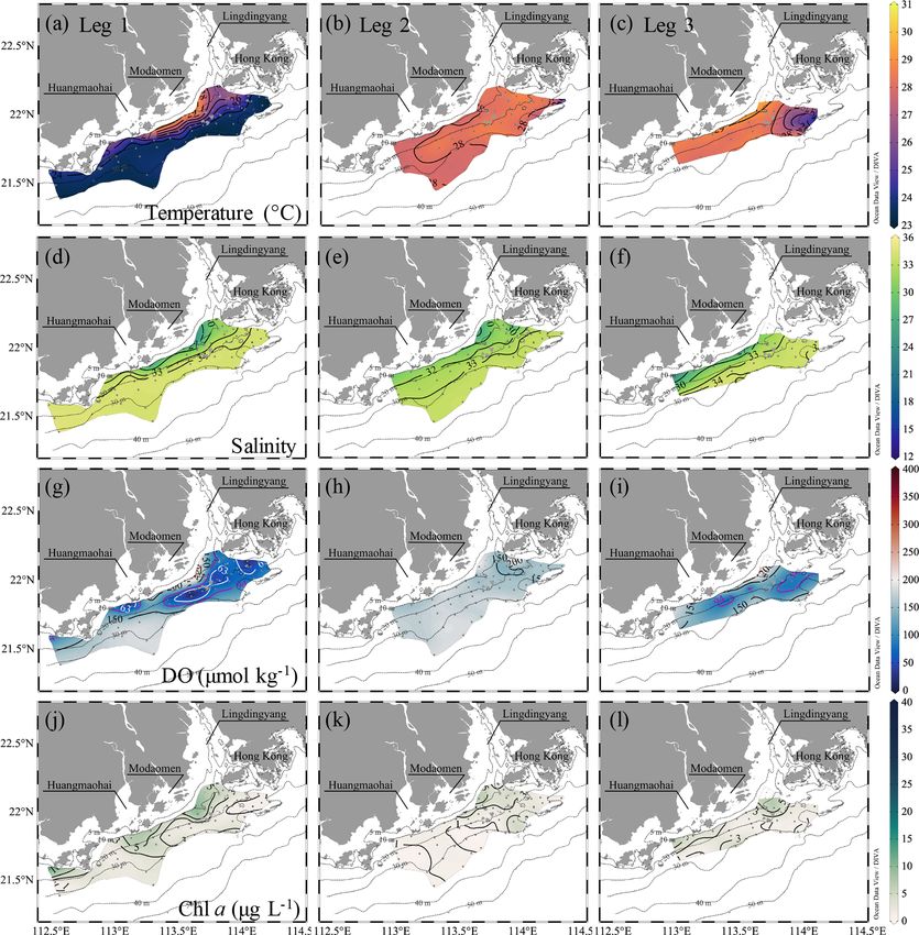
2756                                                         Y. Zhao et al.: Destruction and reinstatement of coastal hypoxia

remains to be better characterized (Testa et al., 2017). Specif-   OCR and timescale for hypoxia regeneration after its destruc-
ically, the identification of key processes and timescale con-     tion by a typhoon. The impacts of tropical cyclones on the
straints for these hypoxia destruction and recovery processes      evolution of seasonal hypoxia in river-dominated ocean mar-
is of critical importance in order to predict site-specific hy-    gins are further discussed.
poxia and its cascading effects and to forecast the long-term
impact of hypoxia under a changing climate with higher-
intensity extreme events (Knutson et al., 2010; Mendelsohn         2     Materials and methods
et al., 2012).
                                                                   2.1    Study area and cruise background
   Large riverine nutrient loadings and the resulting eutroph-
ication have recently tipped the lower Pearl River estuary         The shelf of the northern South China Sea (NSCS) receives
(PRE) and adjacent shelf areas into seasonally hypoxic sys-        an average annual freshwater discharge of ∼ 10 000 m3 s−1
tems (Yin et al., 2004; Rabouille et al., 2008; Su et al., 2017;   originating from the Pearl River, the 17th largest river in the
Qian et al., 2018; Cui et al., 2019; Zhao et al., 2020). Mod-      world (Cai et al., 2004; Dai et al., 2014). Nearly four-fifths
elling results have shown that summer hypoxia off the PRE          of freshwater discharge occurs during the wet season, typi-
is largely intermittent owing to high-frequency variations         cally from April to September (Dai et al., 2014). The riverine
in wind forcing and tidal fluctuations (Wang et al., 2017b;        freshwater extends offshore to form a widespread plume over
Huang et al., 2019). Hypoxia is often interrupted by the pas-      the shelf in summer (Gan et al., 2009b; Cao et al., 2011; Chen
sage of typhoons but redevelops quickly with a tendency to-        et al., 2017a) via eight outlets through three sub-estuaries
wards rapid oxygen declines (Su et al., 2017; Huang et al.,        (i.e. Lingdingyang, Modaomen and Huangmaohai; Fig. 1b).
2019). The prevailing southwest monsoon usually favours            On the inner shelf, coastal upwelling interacts with the buoy-
the expansion of a quasi-steady-state freshwater bulge out-        ant plume, which is propelled by the prevailing southwest
side the entrance of the PRE (Gan et al., 2009b; Lu et al.,        monsoon and intensified along the eastward widened shelf
2018) that promotes water column stability. However, it re-        (Gan et al., 2009a; Chen et al., 2017b). Climatologically,
mains unclear how the interaction between wind stress, tidal       about seven tropical cyclones per year impacted the NSCS
forcing and freshwater buoyancy affects the bottom oxy-            from 1949–2019, half of which featured maximum wind
gen conditions when the winds shift in the downwelling-            speeds greater than 32.7 m s−1 .
favourable easterly or southeasterly direction, especially in         Field observations and sampling were conducted aboard
the wake of tropical cyclones.                                     the R/V Haike 68 off the PRE on the inner-shelf of the NSCS
   It is known that aerobic respiration of organic matter is       in the summer of 2018. The cruise was interrupted by the pas-
largely responsible for the oxygen depletion here (Su et al.,      sage of typhoon Son-Tinh across the NSCS, ∼ 350 km south
2017; Qian et al., 2018). Common methods to quantify oxy-          of the PRE (Fig. 1a). Leg 1 (8–14 July) was the cruise period
gen sinks under hypoxic conditions include the analysis of         before the typhoon, and leg 2 (21–25 July) and leg 3 (26–
oxygen budgets based on the mass balance of oxygen and             29 July) were conducted after its passage (Fig. 1b). During
estimates of community/bacterial respiration or nitrification      each leg, we collected samples from west to east and along
rates using field incubations (Zhang and Li, 2010; Li et al.,      the cross-shelf transects within isobaths of 10–35 m. Almost
2015; Su et al., 2017; Cui et al., 2019). However, the bud-        all stations in leg 1 (56 stations) were revisited during leg 2
get analysis of oxygen typically assumes a steady-state sys-       (56 stations, including 4 stations differing from leg 1) and
tem (Zhang and Li, 2010; Cui et al., 2019) given that the          nearly half again during leg 3 (27 stations). Eight stations
change of oxygen over time is often much smaller than the          were additionally revisited on the way back to the port on
oxygen depletion and advection or diffusion fluxes (Cui et         31 July. Time-series observations with a sampling interval of
al., 2019). The respiration or nitrification rates estimated       1 h were conducted at station F303 for 26 h before leg 2, be-
from (enriched) incubation experiments also merely indicate        ginning at 16:00 UTC+8 on 19 July (Fig. 1b). In contrast to
the oxygen consumption rate (OCR) under a specific low-            the typical southwesterly winds in the NSCS with average
oxygen condition at the time of sampling (He et al., 2014; Su      monthly wind speeds of < 6 m s−1 from June to September
et al., 2017). The actual magnitude of in situ OCR during the      (Su, 2004), easterly winds prevailed during the cruise period
hypoxia formation has rarely been reported at large scales.        due to the typhoon, with the wind speeds increasing up to
The role of lateral advection (and/or upwelling) also remains      ∼ 13 m s−1 (Fig. 1c) at Waglan Island to the east of the study
to be better quantified (Zhang and Li, 2010; Lu et al., 2018;      area (Fig. 1b).
Qian et al., 2018; Cui et al., 2019).
   We investigated the destruction and reinstatement of sum-       2.2    Sampling and analysis
mer hypoxia off the PRE to examine the effects of freshwater
inputs and winds on water column stability and the mainte-         Temperature and salinity were determined using a
nance, destruction and formation of hypoxia. With the aid of       SBE 917 plus conductivity–temperature–depth (CTD)
a three-endmember mixing model, we partitioned physical-           recorder (Sea-Bird Electronics, Inc.). Discrete samples
and biochemical-induced oxygen sinks and calculated the            were collected using 5 L free-flow water samplers mounted

Biogeosciences, 18, 2755–2775, 2021                                                  https://doi.org/10.5194/bg-18-2755-2021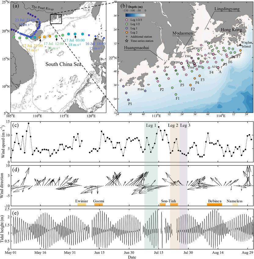
Y. Zhao et al.: Destruction and reinstatement of coastal hypoxia                                                                         2757

Figure 1. (a) Map of the study area on the shelf of the northern South China Sea (NSCS), showing the track of typhoon Son-Tinh (circles)
across the NSCS during 16–24 July 2018. The colour of the circles represents the magnitude of wind speed. Additionally, the smaller circles
denote tropical depression (wind speeds ≤ 17.1 m s−1 ) and the larger circles denote tropical storm (wind speeds within 17.2–32.6 m s−1 ).
The arrows denote the locations of the typhoon as marked with time and wind speed. The grey lines are the depth contours at 50 and 200 m.
(b) Sampling stations on the NSCS shelf off the Pearl River estuary in summer 2018. The pink, green, purple and orange circles denote the
stations surveyed in all three legs, only leg 1 and leg 2, only leg 1, and only leg 2, respectively. Time-series observations were conducted at
station F303 as marked by the star, and vertically high-resolution samplings were conducted at stations marked with bold circles. (c) The
wind speed and (d) wind direction at Waglan Island (triangle in b) from May to August 2018. Bars at the bottom of (d) mark times when
tropical cyclones impacted the NSCS. (e) The tidal height at the Dawanshan gauge station near station F303 from May to August 2018. The
shaded area indicates the cruise periods for leg 1 (grey), leg 2 (pink) and leg 3 (blue).

onto a rosette sampling assembly. Dissolved oxygen (DO),                  layers. Additional high-resolution vertical samplings were
dissolved inorganic carbon (DIC), total alkalinity (TA) and               conducted at seven to eight depth layers (Fig. 1b).
chlorophyll a (Chl a) concentrations were measured at all                    Salinity was calibrated against discrete water samples
stations with depth profiles from 1 m below the surface                   measured by a Multi 340i salinometer (WTW). The DO
down to ∼ 4–6 m above the bottom, generally at three depth                concentrations were measured onboard within ∼ 12 h us-
                                                                          ing the spectrophotometric Winkler method (Labasque et

https://doi.org/10.5194/bg-18-2755-2021                                                            Biogeosciences, 18, 2755–2775, 2021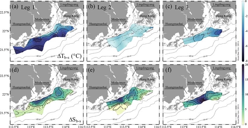
2758                                                         Y. Zhao et al.: Destruction and reinstatement of coastal hypoxia

al., 2004), with a precision better than ± 2 µmol L−1 . DIC        The model is constrained by salinity (S) and potential tem-
was measured on ∼ 0.5 mL acidified water samples using             perature (θ ) according to the following equations:
an infrared CO2 detector (Apollo ASC-3) with a precision
of ± 2 µmol L−1 (Cai et al., 2004). TA was determined on           fPW + fSW + fSUB = 1,                                       (2)
25 mL samples in an open-cell setting based on the Gran            SPW × fPW + SSW × fSW + SSUB × fSUB = S meas ,              (3)
titration technique (see details in Cai et al., 2010) with a       θPW × fPW + θSW × fSW + θSUB × fSUB = θ meas .              (4)
Kloehn digital syringe pump. The analytical precision was
± 2 µmol L−1 . Both DIC and TA concentrations were cali-           where the superscript “meas” denotes measured values, and
brated against certified reference materials provided by An-       f represents the fraction that each endmember contributes to
drew G. Dickson at the Scripps Institution of Oceanography,        the in situ samples. Assuming that DO concentrations in sur-
University of California, San Diego, USA. Chl a concentra-         face waters before sinking to the depth were equilibrated with
tions were determined using a Trilogy laboratory fluorometer       the atmosphere and that the subsurface waters were isolated
(Turner Designs, Inc.) after being extracted with 90 % ace-        from the atmosphere due to restriction by stratification, these
tone for 14 h at −20 ◦ C (Welschmeyer, 1994) and calibrated        fractions were applied to predict conservative concentrations
using a Sigma Chl a standard.                                      of DO (DOmix ) resulting solely from conservative mixing.
                                                                   DOmix = DOPW ×fPW +DOSW ×fSW +DOSUB ×fSUB (5)
2.3    Water column stability
                                                                      Similarly, 1DOmix is the difference in “conservative” DO
Water column stability regulates the ventilation of subsur-        values between visits, assuming that the bottom water masses
face waters and replenishment of DO by suppressing turbu-          where biochemical oxygen consumption prevailed were con-
lent mixing with stratification (Obenour et al., 2012; Lu et       strained by strong convergence and that their outflow from
al., 2018; Cui et al., 2019), which can be indicated by the        the sampling area is insignificant on the timescale of the wa-
buoyancy frequency (also known as the Brunt–Väisälä fre-           ter residence time (Lu et al., 2018; Li et al., 2020). As a re-
quency),                                                           sult,

N 2 = −(g/ρ)(∂ρ/∂z),                                        (1)    OCR = −1DObc /1t = − 1DO − 1DOmix /1t,                      (6)

where g is the gravitational acceleration, ρ is potential den-     where 1t is the duration between the two observations
sity and z is the height above the seabed. Generally, a positive   at times t1 and t2 (t2 >t1 ), and 1X = X t2 − X t1 (X = DO,
N 2 (i.e. N 2 >0 s−2 ) indicates a stable regime where stratifi-   DOmix , DObc , etc.). The uncertainty in the calculation of
cation may suppress turbulence (Tedford et al., 2009), and a       OCR mainly derives from the estimation of conservative
larger N 2 value indicates a more stable water column. CTD         values predicted from the three-endmember mixing model.
temperature and salinity were used to calculate the buoy-          Sources of the composite uncertainty (ε) in derivation of
ancy frequency for sampling stations, to indicate the con-         DOmix are associated with potential temperature (θ ), salinity
trols of density stratification on the development of hypoxia      (S) and the dissolved oxygen (DO) values of endmembers.
(Sect. 4.1).                                                                 r
                                                                               Xn h              2              2 i
                                                                   εDOmix =        i
                                                                                      f i · σDOi    + DO i · σfi     ,        (7)
2.4    Oxygen consumption rate
                                                                   where σDO and σf are uncertainties in the DO concentra-
From the perspective of Euler observations and based on
                                                                   tion and the fraction of each endmember i (i.e. PW, SW and
mass balance, the DO changes (1DO) in subsurface waters
                                                                   SUB), respectively, and the latter of which can be calculated
over a specified time interval at a specific site can be decom-
                                                                   as
posed into two components: one driven by physical mixing                 r
(1DOmix ) and the other induced by biochemical processes                   Xn h                      2                   2 i
                                                                   σfi =           ∂f i /∂θ j · σθ      + ∂f i /∂Sj · σS      , (8)
(1DObc ). Here, we define the biochemical-induced DO con-                      j                   j                    j

sumption with time as the oxygen consumption rate (OCR).           where j also denotes each endmember.
A higher OCR value indicates stronger oxygen consumption,
and a negative value indicates oxygen production via bio-          2.5   Endmember selection and validations of the
chemical processes (e.g. photosynthesis). For revisited sta-             three-endmember mixing model
tions, 1DO is the difference in DO values measured between
the two sampling periods. The physical-mixing-induced DO           The potential-temperature–salinity diagram is shown in
variations were derived using a three-endmember mixing             Fig. 2a. The three-endmember mixing scheme for the bottom
model, which constructed the conservative mixing scheme            layer has been elucidated in Zhao et al. (2020) that had a spa-
among different water masses: brackish plume water (PW),           tial coverage similar to this study. We adopted the endmem-
offshore surface water (SW) and upwelled subsurface water          ber values of the offshore surface water and upwelled subsur-
(SUB) (Su et al., 2017; Cui et al., 2019; Zhao et al., 2020).      face water from Zhao et al. (2020) given that our sampling

Biogeosciences, 18, 2755–2775, 2021                                                   https://doi.org/10.5194/bg-18-2755-2021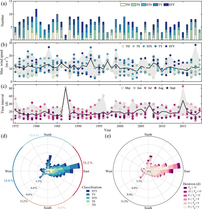
Y. Zhao et al.: Destruction and reinstatement of coastal hypoxia                                                          2759

was almost exclusively within the 30 m isobaths (Fig. 1b),       2009b; Lu et al., 2018). A strong bloom occurred in the sur-
and these values were consistent with those found in previ-      face plume waters near the Huangmaohai sub-estuary, char-
ous studies (Cao et al., 2011; Guo and Wong, 2015; Su et         acterized by high Chl a concentrations of >20 µg L−1 and
al., 2017). The brackish plume water was assumed to partly       oversaturated DO of >300 µmol kg−1 (equivalent to a DO
subduct to the bottom layer under downwelling-favourable         saturation level >150 %) (Fig. 3g, j). The freshwater bulge
wind conditions (Huang et al., 2019; Li et al., 2021). The       also featured a relatively weak bloom, with Chl a concen-
endmember values of the brackish plume water were thus           trations of ∼ 10 µg L−1 and DO of ∼ 250 µmol kg−1 (equiv-
determined from the surface water samples near the mouth         alent to a DO saturation level of ∼ 125 %). Similar blooms
of the PRE with a salinity of ∼ 16.9, mainly consisting of       were previously observed to be associated with high nutri-
a mixture of riverine freshwater and offshore surface water.     ent concentrations, a sufficiently long water residence time
The DIC endmember of brackish plume water here was con-          and an abundance of photosynthetically active radiation (Lu
sistent with the predicted value using the endmember values      and Gan, 2015). The surface water temperature was mostly
of riverine/plume water reported by Su et al. (2017), whereas    >29 ◦ C. Exceptions occurred to the southwest of Hong Kong
it was higher than that calculated using the endmember val-      (Fig. 3a) where the air temperature was 2–3 ◦ C lower at the
ues of riverine freshwater from Zhao et al. (2020) since the     time of sampling (Fig. S1 in the Supplement).
riverine DIC concentrations might be diluted by abnormally          At the bottom layer, low-temperature (< 26 ◦ C), high-
high river discharge in 2017 (Guo et al., 2008). For simpli-     salinity (>33) deep shelf waters intruded upslope to the 10–
fication, DO concentrations in offshore surface water were       20 m isobaths beneath the surface plume (Fig. 4a, d). An
assumed to be saturated, in equilibrium with the atmosphere,     extensive hypoxic zone (DO < 63 µmol kg−1 ) developed be-
while the upwelled subsurface water was assumed to be oxy-       neath the freshwater bulge and extended westwards along
gen deficient by ∼ 16 % relative to the saturation level. The    the 20–30 m isobaths to the region off the Modaomen sub-
DO endmember value of brackish plume water was also as-          estuary (Fig. 4g). To the east, a relatively weak hypoxic cen-
sumed to be equilibrated with the atmosphere, which should       tre occurred adjoining the Hong Kong waters. Additionally,
be in order, because the biological productivity was largely     a smaller-scale hypoxic zone appeared beneath the surface
limited by high turbidity in shallow estuarine waters. A sum-    bloom near the Huangmaohai sub-estuary, a region where
mary of the endmember values is listed in Table 1. In esti-      hypoxia was also reported but not fully covered by survey
mating the OCR, we excluded the above-pycnocline samples         measurements (Su et al., 2017; Cui et al., 2019). The gen-
collected at depths < 10 m affected by the upper plume wa-       eral spatial pattern of hypoxic centres was similar to that
ters that are subject to strong air–sea exchanges and/or pho-    found in summers of 2014 and 2017 (Su et al., 2017; Zhao
tosynthetic production of oxygen.                                et al., 2020) yet with a slight offshore shift. The minimum
   The predicted quasi-conservative TA (TApre = TAPW ×           oxygen level was 3.5 µmol kg−1 (∼ 0.1 mg L−1 ) in bottom
fRW + TASW × fSW + TASUB × fSUB ; same for DICpre ) is           waters at station F303, which was lower than the previ-
mostly consistent with our measured values (Fig. 2b),            ously reported minimum (∼ 7 µmol kg−1 at station F304; Su
with a subtle difference of 8 ± 8 µmol kg−1 likely as-           et al., 2017). Within the surveyed region where DO con-
sociated with measurement errors, computational er-              centrations were interpolated into 0.50 × 0.50 grids using the
rors in the mixing scheme and/or biological processes.           Kriging interpolation method, the total area of the hypoxic
The slope of 1DIC (1DICm−p = DICmeas − DICpre ) vs.              zone reached ∼ 660 km2 , and the oxygen-deficit zone (DO
1DOm−p (1DOm−p = DOmeas − DOmix ) in bottom waters               < 94 µmol kg−1 ) occupied ∼ 1470 km2 , which was larger
was −0.93 ± 0.07 (Fig. 2c), similar to that reported by Zhao     than those in summer 2014 (>280 km2 for the hypoxic zone
et al. (2020).                                                   and >800 km2 for the oxygen-deficit zone) when we sur-
                                                                 veyed in a smaller area (Su et al., 2017). Cui et al. (2019)
                                                                 reported that spring–neap tidal oscillations lead to varia-
3     Evolution of intermittent hypoxia off the PRE              tions in the DO concentration outside of the Lingdingyang
                                                                 sub-estuary with a maximum neighbouring oxygen range of
3.1    Extensive hypoxia before the typhoon                      ∼ 15 µmol kg−1 . As our observations were conducted during
                                                                 the transition from the neap tide to the spring tide (Fig. 1e),
The water columns showed a prominent two-layer structure         the total areas of the hypoxic zone and the oxygen-deficit
on the inner NSCS shelf off the PRE (Figs. 3 and 4). In          zone would be at most ∼ 990 and ∼ 1930 km2 , respectively,
the surface layer, the freshwater plume mainly attached to       which are 34 %–50 % larger than our observed areas.
the coast when veering to the west as constrained by es-
tuarine topography, the Coriolis force (Wong et al., 2003)       3.2   Destruction of hypoxia by the typhoon
and easterly winds during leg 1 (Fig. 1d), despite a freshwa-
ter bulge that remained near the mouth of the Lingdingyang       The spatial patterns of temperature, salinity, DO and Chl a
sub-estuary due to persistent southwesterly winds before the     concentrations all changed drastically from disturbance by
cruise (Fig. 1d) and the weak shelf current there (Gan et al.,   intensified easterly winds during the typhoon period. Strong

https://doi.org/10.5194/bg-18-2755-2021                                                 Biogeosciences, 18, 2755–2775, 2021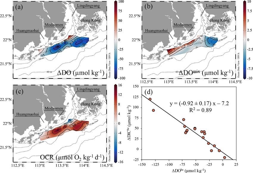
2760                                                                        Y. Zhao et al.: Destruction and reinstatement of coastal hypoxia

Figure 2. (a) Potential temperature (◦ C) vs. salinity, (b) predicted TA (TApre , µmol kg−1 ) vs. measured TA (TAmeas , µmol kg−1 )
and (c) 1DICm−p (µmol kg−1 ) vs. 1DOm−p (µmol kg−1 ) on the NSCS shelf off the PRE. The black-edged circles represent bottom
water samples with depths >10 m. The yellow, green and purple triangles in (a) represent the endmember values of brackish plume water
(PW), offshore surface water (SW) and upwelled subsurface water (SUB), respectively. The black line in (c) denotes the slope of 1DICm−p
plotted against 1DOm−p derived from the Model II regression.

Table 1. Summary of the endmember values adopted in the three-endmember mixing model.

                    Water mass                                    θ (◦ C)         Salinity      DIC (µmol kg−1 )          DO (µmol kg−1 )
                    Brackish plume water                    28.9 ± 0.4b              16.9              1776 ± 29b               217.3 ± 1.4c
                    Offshore surface watera                  29.3 ± 0.1        33.7 ± 0.1                1922 ± 5               194.4 ± 0.3c
                    Upwelled subsurface watera               22.5 ± 0.1        34.5 ± 0.0                2022 ± 3               180.9 ± 0.4c
                  a Adopted from Zhao et al. (2020). b Uncertainties were derived from multiple samples collected at the entrance of the PRE.
                  c Uncertainties were calculated by propagating errors associated with the estimation of oxygen solubility using Benson and
                  Krause (1984).

winds drove the warm, low-salinity and oxygen-saturated                              was ∼ 29.0 ± 0.5 ◦ C, which was higher than that in bottom
surface waters to mix downward, increasing temperature and                           waters by 0.8 ◦ C during leg 2 (Figs. 3b and 4b).
DO concentrations and decreasing salinity in bottom wa-                                 In bottom waters, hypoxia had been completely de-
ters (Fig. 4). Time-series observations at station F303 before                       stroyed due to strong reaeration in the wake of the ty-
leg 2 showed a vertically well-mixed water column in the                             phoon travelling across the NSCS, replaced by a homoge-
first half, as reflected by homogeneous distributions of inter-                      nous spatial distribution of relatively high DO concentra-
mediate temperature (∼ 28 ◦ C), salinity (∼ 32) and DO lev-                          tions (∼ 171 ± 16 µmol kg−1 ) during leg 2 (Fig. 4h). The
els (∼ 180 µmol kg−1 ) (Fig. 5a–c). The less well-mixed wa-                          cross-shore gradients in temperature and salinity were also
ter column in the second half of the time-series observations                        largely relaxed, with isotropically elevated temperatures up
likely resulted from the weakened winds, showing an up-                              to ∼ 28 ◦ C and decreased salinity (Fig. 4b, e). The mid-depth
ward intrusion of bottom waters which were slightly warmer                           distributions of temperature, salinity and DO concentrations
than surface waters which lost heat to the low-temperature                           showed similar patterns as at the bottom layer (Fig. S2).
atmosphere (Fig. S1). With subdued winds that shifted to                             Although the water column remained relatively well-mixed
southwesterly in the following 2 d (Fig. 1c, d), the offshore                        in the subsurface layer, freshwater buoyancy and weakened
spreading of the river plume suppressed the upward intrusion                         winds facilitated the revitalization of density stratification
of slightly warm bottom waters and facilitated the restora-                          and subsequent oxygen decline below the pycnocline. In-
tion of a two-layer water column, as observed in the second                          deed, the bottom water DO concentration at station F303
half of the time-series observations (Fig. 5) and during leg 2                       decreased by ∼ 18 µmol kg−1 compared to that in the time-
(Figs. 3 and 4). Large phytoplankton blooms were identified                          series observations and was lower than that at adjacent sta-
in the surface plume, widely spreading from the mouth of                             tions by ∼ 9–22 µmol kg−1 when revisited during leg 2 on
the Lingdingyang sub-estuary to near the Huangmaohai sub-                            22 July (Fig. S3).
estuary (Fig. 3k), potentially fuelled by nutrients mixed up-
ward from the depth in addition to riverine inputs (Wang et                          3.3     Reinstatement of hypoxia after the typhoon
al., 2017b; Qiu et al., 2019). The maximum Chl a concen-
tration was >40 µg L−1 off the Modaomen sub-estuary, ac-                             With the dying out of the typhoon after its landfall to the
companied by an extraordinarily high DO concentration of                             west of the study area on 23 July (Fig. 1a), the wind speed
>350 µmol kg−1 (Fig. 3h, k). The surface water temperature                           decreased to < 5 m s−1 on 25 July, while the wind direction

Biogeosciences, 18, 2755–2775, 2021                                                                            https://doi.org/10.5194/bg-18-2755-2021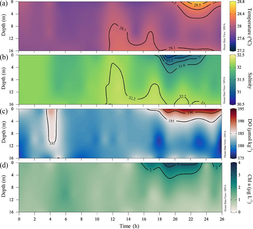
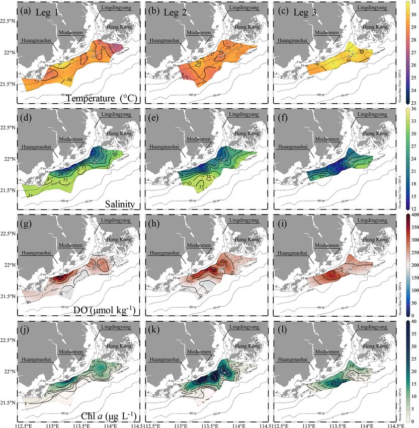
Y. Zhao et al.: Destruction and reinstatement of coastal hypoxia                                                                       2761

Figure 3. Distributions of temperature (◦ C), salinity, DO (µmol kg−1 ) and Chl a concentrations (µg L−1 ) at the surface water layer off the
PRE during pre-typhoon leg 1 and during post-typhoon legs 2 and 3. The white and magenta contours in (g) and (w) show the hypoxic
(DO < 63 µmol kg−1 ) and oxygen-deficit (DO < 94 µmol kg−1 ) zones, respectively. Figures were produced using Ocean Data View v. 5.3.0
(http://odv.awi.de, last access: 8 June 2020, Schlitzer, 2018).

remained from the southeast before it shifted to southwest-              surface layer was warmed up to over 30 ◦ C (Fig. 3c), increas-
erly on 29 July (Fig. 1c, d). The DO concentrations in bot-              ing vertical thermal gradients relative to leg 2 (Figs. 3 and 4)
tom waters were noticeably lower (139–164 µmol kg−1 shal-                and strengthening the stratification (Allahdadi and Li, 2017).
lower than 20 m isobaths), starting around July 23 in the sec-           The freshwater bulge of lower salinity (< 15) advected off-
ond half of leg 2 (Figs. 1b and 4h). During leg 3 from 26–               shore around the Modaomen sub-estuary, with the offshore
29 July, hypoxia was present again in bottom waters, due to              migration of the bloom (Fig. 4f, l) likely driven by the inter-
favourable conditions for its formation (Figs. 3 and 4). The             action between the seaward buoyant current and northeast-

https://doi.org/10.5194/bg-18-2755-2021                                                           Biogeosciences, 18, 2755–2775, 2021
2762                                                            Y. Zhao et al.: Destruction and reinstatement of coastal hypoxia

Figure 4. Distributions of temperature (◦ C), salinity, DO (µmol kg−1 ) and Chl a concentrations (µg L−1 ) at the bottom water layer off the
PRE during pre-typhoon leg 1 and during post-typhoon legs 2 and 3. The white and magenta contours in (g) and (w) show the hypoxic
(DO < 63 µmol kg−1 ) and oxygen-deficit (DO < 94 µmol kg−1 ) zones, respectively.

ward shelf current (Pan et al., 2014; Li et al., 2020). The             (Huang et al., 2019; Li et al., 2021), augmenting temper-
Chl a concentrations near the entrances of the three sub-               ature and DO concentrations but bringing down salinity,
estuaries remained relatively high (>10 µg L−1 ), and the DO            particularly in the mid-depth layer from 3–5 m at stations
concentrations remained at high levels of >250 µmol kg−1 ,              nearest the shore to ∼ 15 m at stations furthest from the
which were ∼ 20 % over the saturation levels (Fig. 3i, l).              shore (Fig. S2). The downward penetration of surface wa-
   Similar to leg 1 and leg 2, the surface waters pene-                 ters, nonetheless, seemed to be restricted to the ∼ 10 m iso-
trated into the subsurface layer along the coast (Fig. 4f),             bath and thus offset only a limited amount of the oxygen
likely forced by the downwelling-favourable winds (Fig. 1d)             reduction caused by biochemical consumption (Koweek et

Biogeosciences, 18, 2755–2775, 2021                                                         https://doi.org/10.5194/bg-18-2755-2021
Y. Zhao et al.: Destruction and reinstatement of coastal hypoxia                                                                          2763

Figure 5. Time-series observations of (a) temperature (◦ C), (b) salinity, (c) DO (µmol kg−1 ) and (d) Chl a concentrations (µg L−1 ) at station
F303 (see Fig. 1b) from 19–20 July 2018 after the typhoon passage, showing the complete destruction and the subsequent rapid development
of stratification.

al., 2020). DO concentrations in bottom waters were reduced               4     Physical and biogeochemical controls on the
to ∼ 46 µmol kg−1 off the Modaomen sub-estuary along the                        evolution of intermittent hypoxia
20 m isobaths and to < 94 µmol kg−1 to the southwest of
Hong Kong (Fig. 4i), indicating the reinstatement of hy-                  4.1    Water column stability
poxia. When sites were revisited on 31 July, the re-emerging
hypoxia was found to have been strengthened, with oxy-
                                                                          A stable water column is a key prerequisite for the forma-
gen levels down to ∼ 37 µmol kg−1 . We found that hypoxia
                                                                          tion and maintenance of hypoxia in coastal oceans (Wang and
formed in bottom waters with a temperature of ∼ 28 ◦ C off
                                                                          Justić, 2009; Obenour et al., 2012; Testa and Kemp, 2014; Lu
the Modaomen sub-estuary during leg 3, while the oxygen-
                                                                          et al., 2018; Zhang et al., 2019), which restricts the oxygen
deficit zone to the southwest of Hong Kong showed a rela-
                                                                          supply by suppressing advective and diffusive mixing with
tively low temperature of < 27 ◦ C (Fig. 4c), likely due to the
                                                                          oxygen-rich waters (Murphy et al., 2011; Cui et al., 2019).
cross-isobath transport of deep shelf waters, arising from lo-
                                                                          Many studies have demonstrated that density stratification
cal topographic effects (Dai et al., 2014; Wang et al., 2014)
                                                                          becomes enhanced and stabilizes subsurface waters when
as during leg 1. In this sense, the shoreward intrusion of deep
                                                                          freshwater flows over seawater (Gan et al., 2009b; Mac-
shelf waters is not a prerequisite for the initiation of hypoxia
                                                                          Cready et al., 2009; Bianchi et al., 2010), allowing oxygen
formation off the PRE, but it contributes to the reinstatement
                                                                          depletion over a longer timescale (Fennel and Testa, 2019).
of hypoxia southwest off Hong Kong.
                                                                          In the second half of the time-series observations, the two-
                                                                          layer structure re-emerged with the spreading of the river
                                                                          plume, which suppressed the vertical mixing in the subsur-

https://doi.org/10.5194/bg-18-2755-2021                                                             Biogeosciences, 18, 2755–2775, 2021
2764 Y. Zhao et al.: Destruction and reinstatement of coastal hypoxia face layer, as reflected by the receded upward intrusion of driven by freshwater inputs and the inherent thermocline and slightly warm, saline bottom waters (Fig. 5a, b). The Chl a resulted in a vertically well-mixed water column (Fig. 5). concentrations in the surface layer increased, followed by The surface waters became undersaturated (∼ 90 % of the an elevated DO level in surface waters and a lowered DO oxygen saturation level) due to the upward mixing of low- level in subsurface waters (Fig. 5c, d). The surface-to-bottom oxygen waters, which in turn favoured the ventilation of bot- salinity difference showed large values within the surface tom waters and the breakdown of hypoxic conditions (Hu plume area, which almost covered the bottom hypoxic zones et al., 2017). Despite wind speeds still as high as 10 m s−1 (Fig. 4g, i). Exceptions only occurred to the hypoxic zone during leg 2 (Fig. 1c), stratification was regenerated in the off the Modaomen sub-estuary, where the surface-to-bottom top ∼ 10 m of the plume region, which had relatively large salinity differences were relatively small but the tempera- surface-to-bottom salinity differences (Fig. 6e) and high N 2 ture differences were large (i.e. 1Tb−s < −4 ◦ C in Fig. 6a– (Fig. 7e–h) under easterly winds (Fig. 1d). This suggests that c) due to the shoreward intrusion of cold deep shelf wa- freshwater input-induced stratification suppressed turbulent ters (Fig. 4a–c). The regions occupied by the surface plume mixing driven by wind stress, favouring the initiation of hy- and the shoreward-intruded deep shelf waters therefore over- poxia development even under downwelling-favourable con- lapped, resulting in a more stable water column where a ditions. Most modelling work simulated the formation of hy- patchy hypoxic zone could persist for more than 5 d (Cui et poxia off the PRE under the typical summer southwest mon- al., 2019). soon (Wei et al., 2016; Lu et al., 2018; Li et al., 2020; Yu Off the PRE, when not influenced by freshwater in- et al., 2020); when southwest winds blow in a more south- puts, the surface layer showed a relatively small N 2 close ward direction, a larger hypoxic zone develops (Wei et al., to 0 s−2 and vertically well-mixed temperature, salinity 2016). In contrast to southwesterly winds that facilitate the and DO concentrations (e.g. in the top ∼ 10 m at station wide eastward spreading of the surface plume (Gan et al., A14, Fig. 7c). However, in the presence of the freshwa- 2009b), the downwelling-favourable easterly winds tend to ter plume, the surface layer became more stable, with a constrain the surface plume to flow westward near the coast larger N 2 of >1 × 10⁻³ s−2 , or even >5 × 10⁻³ s−2 (e.g. (Li et al., 2021) as shown during leg 2 and even drive the stations A8 and A11, Fig. 7a, b). The DO concentrations surface oxygen-saturated waters to penetrate into the deep decreased sharply at the base of the surface plume (salin- along the coast (Figs. S2 and 4), resulting in an offshore or ity ∼ 30). Using the eddy diffusivity for density (Kz ) of westward shift of the hypoxic zones that only partly over- < 5 × 10⁻⁶ m2 s−1 for N 2 larger than 1 × 10⁻³ s−2 (Cui et lapped with the surface plume in terms of their localities. If al., 2019), we estimated the vertical diffusion for DO con- the easterly winds last for a longer time than the hypoxia centrations (VDIF = Kz × (∂DO / ∂z)) of ∼ 0.25 g m−2 d−1 formation timescale, stronger blooms in the surface plume with a maximum of 0.54 g m−2 d−1 in the top 10 m at stations (Fig. 3k) would enhance the bottom hypoxia with abundant A8 and A11, which was comparable to the results from Cui supply of fresh, labile organic matter, but the downwelling- et al. (2019). It therefore acted as a barrier layer, with weak favourable winds would also destroy the bottom hypoxia if dissipation of oxygen into the subsurface waters. The inher- the wind stresses become strong enough (Li et al., 2021). ent pycnocline between the offshore surface water and deep shelf waters mainly driven by steep temperature gradients 4.2 Oxygen sinks and hypoxia formation timescale (Qu et al., 2007), such as at station A14, acted as a second pycnocline in the plume region (e.g. stations A8 and A11, 4.2.1 Mixing-induced oxygen sinks Fig. 7a) yet with weaker stratification likely from increased shear stresses in shallower waters (Pan and Gu, 2016; Li et With the restoration of density stratification from leg 2 to al., 2020). At the edge of the freshwater plume (Figs. 1b and leg 3, DO concentrations in bottom waters were gener- 3a), such as station F304, the second pycnocline was more ally reduced by >25 µmol kg−1 , with two hotspots show- stable than that induced by freshwater inputs (Fig. 7d). This ing reductions up to 75 µmol kg−1 : one located offshore of three-layer structure, separated by two pycnoclines, therefore the Lingdingyang sub-estuary, to the southwest of Hong effectively decreased oxygen influx from the surface and fa- Kong, and the other between the Modaomen and Huang- cilitated oxygen depletion in bottom waters. maohai sub-estuaries (Fig. 8a). The mixing-induced DO Water column stability also largely depends on wind stress changes were positive along the coast within 10–20 m iso- and/or direction in coastal waters (Wilson et al., 2008; Wang baths, as the oxygen-saturated surface waters penetrated and Justić, 2009). Higher wind stress usually de-stratifies the downward to re-aerate the bottom waters driven by the water column, leading to stronger turbulent mixing, air–sea downwelling-favourable easterly winds (Huang et al., 2019). gas exchange and reaeration (Chen et al., 2015; Lu et al., The mixing-induced oxygen sinks mainly occurred in bot- 2018; Huang et al., 2019), relieving hypoxic conditions (Ni tom waters southwest off Hong Kong, with an average et al., 2016; Wei et al., 2016). During the typhoon period, the of −5.7 ± 0.8 µmol kg−1 , which was higher than in other wind speed rose to as high as 13 m s−1 (Fig. 1c), which was regions west of the PRE (e.g. beyond the 20 m isobath; large enough to break the stratification (Geng et al., 2019) −1.4 ± 0.8 µmol kg−1 ) (Fig. 8b). The mixing-induced oxy- Biogeosciences, 18, 2755–2775, 2021 https://doi.org/10.5194/bg-18-2755-2021
Y. Zhao et al.: Destruction and reinstatement of coastal hypoxia                                                                  2765

Figure 6. The surface-to-bottom temperature (a–c) and salinity (d–e) distributions off the PRE during pre-typhoon leg 1 and post-typhoon
during legs 2 and 3. 1Tb−s and 1Sb−s represent the difference in temperature and salinity, respectively, between the bottom and surface
layer.

gen sinks can be attributed to the shoreward intrusion of             ration when the source waters transited shoreward over the
oceanic, cold oxygen-undersaturated subsurface waters – as            shelf. Comparing with these systems, the source water orig-
reflected by lowered temperature (< 27 ◦ C; Fig. 4c), which           inating from the low-latitude high-temperature oligotrophic
usually act as a non-local driver of coastal hypoxia by low-          NSCS (Wong et al., 2007) has a higher DO level (AOU
ering the initial DO concentration (Wang, 2009; Qian et al.,          ∼ 35 µmol kg−1 ). As the NSCS shelf is narrower than the
2017). The cold, saline oceanic subsurface waters also com-           East China Sea shelf, the source water spends a shorter time
pletely occupied the bottom layer beyond the 20 m isobath             intruding towards the coastal zone after diverting its direction
during leg 1, where extensive hypoxia developed (Fig. 4a,             from the continental slope (Gan et al., 2009a; Wang et al.,
g). This upwelling-induced reduction in the initial DO level          2014). These might explain the relatively low contribution of
amounted to 8.6 ± 1.7 % of the oxygen decline to the south-           coastal upwelling to the oxygen depletion on the inner NSCS
west of Hong Kong, suggesting coastal upwelling played a              shelf off the PRE.
minor role in the hypoxia formation.
   The contribution of oxygen-deficient coastal upwelling to          4.2.2   Biochemical-induced oxygen sinks
the hypoxia formation varies in different ocean marginal sys-
tems, which is largely dependent on the source of the subsur-         The biochemical-induced DO and DIC changes from leg 2
face water masses and biogeochemical reactions along the              to leg 3 also showed a good relationship with a slope
pathway of the intrusion. Qian et al. (2017) showed the ap-           of −0.92 ± 0.17 (Fig. 8d), consistent with the slope of
parent oxygen utilization (AOU) values of ∼ 50 µmol kg−1              biochemical-induced variations in DO against DIC con-
in the source waters of the nearshore Kuroshio branch at              centrations throughout the sampling legs (Fig. 2c), im-
the shelf break northeast of Taiwan and an AOU increment              plying that aerobic respiration of organic matter indeed
of ∼ 40 µmol kg−1 throughout its travel time of ∼ 60 d to             dominated the oxygen consumption. The distribution of
the vicinity off the Changjiang river (Yang et al., 2013). In         OCR estimates in bottom waters almost mirrored vari-
eastern boundary upwelling systems along the northeast Pa-            ations in the total DO pattern from leg 2 to leg 3
cific Ocean, the source waters typically have a low DO con-           (Fig. 8a, c). This biochemically mediated OCR ranged from
centration of ∼ 80–160 µmol kg−1 , even near or below hy-             0.9 µmol O2 kg−1 d−1 at offshore non-hypoxic stations to
poxic levels from a depth of ∼ 100–200 m (Grantham et al.,            19.5 ± 0.4 µmol O2 kg−1 d−1 in hypoxic waters, with an av-
2004). The DO deficits were further exacerbated by respi-             erage of 14.6 ± 4.8 µmol O2 kg−1 d−1 in the oxygen-deficit
                                                                      zone. The uncertainty introduced by the mixing scheme was

https://doi.org/10.5194/bg-18-2755-2021                                                       Biogeosciences, 18, 2755–2775, 2021
2766 Y. Zhao et al.: Destruction and reinstatement of coastal hypoxia Figure 7. Profiles of temperature (◦ C) (blue dashed lines), salinity (pink solid lines), dissolved oxygen (DO, µmol kg−1 ) (purple dots) and buoyancy frequency N 2 (s−2 ) (bold black solid lines) at stations A8, A11, A14 and F304 (see Fig. 1b), with visits for both pre-typhoon (leg 1) and post-typhoon periods (legs 2 and 3). The vertical distributions of N 2 have been smoothed by the Gaussian method. 0.63–0.98 µmol O2 kg−1 d−1 , accounting for a deviation of wedge (Zhang and Li, 2010) to fuel the high OCR there. In 4 %–27 %. The geographical locations of high-OCR zones fact, only the west hypoxic centre was located beneath the at the bottom layer (OCR >10 µmol O2 kg−1 d−1 ) were not surface bloom from leg 2 to leg 3 (Figs. 3j–l and 4g–i). Lu fully overlapped with those of surface blooms (Figs. 3l and et al. (2018) proposed another explanation that small detritus 8c). Cui et al. (2019) suggested that the patchy distribu- of external sources could be accumulated and remineralized tion of bottom hypoxia was closely associated with the river in the bottom flow convergence zone as regulated by highly plume front which traps organic particles (Hetland and Di- variable coastline and bottom topography. Our observed hy- Marco, 2008), accelerating their settlement and deposition in poxic zones generally coincided with the modelled strong the overlapping zones between the river plume and shelf salt convergence zones (Lu et al., 2018; Li et al., 2020), imply- Biogeosciences, 18, 2755–2775, 2021 https://doi.org/10.5194/bg-18-2755-2021
Y. Zhao et al.: Destruction and reinstatement of coastal hypoxia                                                               2767

Figure 8. Distributions of (a) total DO changes (1DO, µmol kg−1 ), (b) mixing-induced DO changes (1DOmix , µmol kg−1 ) and (c) the
biochemical-induced oxygen consumption rate (OCR, µmol O2 kg−1 d−1 ) between leg 3 and leg 2 on the inner NSCS shelf off the PRE. (d)
The biochemical-induced changes in DIC (1DICbc , µmol kg−1 ) vs. DO (1DObc , µmol kg−1 ) in bottom waters with depths >10 m from
leg 2 to leg 3. The black line denotes the slope of 1DICbc plotted against 1DObc derived from the Model II regression.

ing sufficient organic matter supply fuelled the high OCR to         For stations with the middle layer also below the pycnocline,
restore hypoxia in bottom waters.                                    such as station F304 during leg 3, the profile of DO concen-
   Our estimated OCR is comparable in magnitude to the               trations showed almost constant values below the pycnocline
community/bacterial respiration rate from previous stud-             (Fig. 7k). Sediment oxygen demand might be significant near
ies in this study area (9.6 µmol O2 kg−1 d−1 ; Su et al.,            the seabed or in its overlying water column in shallow wa-
2017; 7.9 to 19.0 µmol O2 kg−1 d−1 ; Cui et al., 2019;               ters (Kemp et al., 1992; Zhang and Li, 2010). However, our
16.8 ± 8.9 µmol O2 kg−1 d−1 ; Li et al., 2019) and within the        sampling at the bottom layer was 4–6 m above the seabed,
range in other estuaries and coastal systems (Dortch et al.,         and the water depth of the hypoxic zones was nearly 20 m
1994; Robinson, 2008), despite a lower limit due to a po-            (Fig. 4). In such sampling areas, Cui et al. (2019) found that
tential overestimation of the actual time if significant oxy-        oxygen losses by sediment oxygen demand (i.e. benthic res-
gen consumption started later than our observations during           piration) were much smaller than the bacterial respiration in
the first half of leg 2 and an assumed negligible oxygen flux        the water column based on both incubation experiments and
supplied from the surface by diffusion. From leg 2 to leg 3,         oxygen budget analysis. We thus assumed the sediment oxy-
the vertical oxygen diffusion flux was ∼ 0.18 g m−2 d−1 ,            gen demand was negligible and the microbial respiration in
amounting to a supply of ∼ 0.6–1.1 µmol O2 kg−1 d−1 to the           the water column dominated the estimated OCR.
bottom waters with a thickness of 5–10 m. The exclusion of              However, the estimated OCR here differs in implications
this vertical oxygen diffusion flux in our estimates therefore       from that derived from the steady-state budget analysis in
might underestimate the OCR by ∼ 6 % on average. We also             which the oxygen consumption was completely offset by the
assumed that the OCR was uniform in the subsurface waters            physical transport of oxygen (Zhang and Li, 2010; Cui et al.,
several metres above the seabed, because we collected sam-           2019). In our estimates, the OCR was derived during the hy-
ples at three depth layers during leg 2 and leg 3, with usu-         poxia formation in which the in situ DO concentrations de-
ally only one layer below the pycnocline for most stations.          creased over time (i.e. in a non-steady-state system) as oxy-

https://doi.org/10.5194/bg-18-2755-2021                                                     Biogeosciences, 18, 2755–2775, 2021
2768                                                       Y. Zhao et al.: Destruction and reinstatement of coastal hypoxia

gen sinks exceed sources. To shift from such a non-steady-       hypoxia formation timescales are shorter than the bottom
state system towards a balance between oxygen consump-           water residence time (>15 d, Li et al., 2020), which favoured
tion and replenishment for the maintenance of hypoxia, the       the hypoxia formation to the west off the PRE (Su et al.,
OCR might decrease or the physical-induced oxygen supply         2017; Zhao et al., 2020).
increases. Kalvelage et al. (2015) found that aerobic respi-        For a more common scenario of hypoxia formation start-
ration rates decreased with decreasing in situ DO concentra-     ing from late spring, we assumed that the shoreward-intruded
tions, i.e. from the upper boundary of oxygen minimum zone       oxygen-deficient offshore subsurface waters almost occu-
(OMZ) towards the OMZ core off Peru. The oxygen enriched         pied the bottom layer on the inner shelf instead of the well-
incubation of unfiltered water samples revealed that the OCR     oxygenated offshore surface waters, as during leg 1 (Fig. 4a,
changed little when the in situ DO concentration was higher      d). Based on the above estimates that the shoreward-intruded
than ∼ 90 µmol kg−1 but also decreased when the in situ DO       subsurface waters totally reduced the initial DO level by
concentration decreased to ∼ 30 µmol kg−1 (He et al., 2014).     8.6 ± 1.7 % of the oxygen decline for hypoxia formation,
Despite the bottom DO concentrations of ∼ 180 µmol kg−1          the initial DO level was lowered by ∼ 11 µmol kg−1 to be
at station F303 during the time-series observations, DO de-      ∼ 183 µmol kg−1 before biochemical oxygen consumption.
clined at a rate of ∼ 9 µmol O2 kg−1 d−1 from 20–22 July,        The hypoxia hotspot will then first occur ∼ 6 d after its ini-
when the winds remained strong, and the OCR decreased            tiation on the inner NSCS shelf off the PRE and extend to a
to ∼ 5.5 µmol O2 kg−1 d−1 from leg 2 (DO ∼ 164 µmol kg−1 )       larger hypoxic zone within the water residence time of >15 d
to leg 3 (DO ∼ 127 µmol kg−1 ) (from 22–29 July) (Fig. S3).      (Lu et al., 2018; Li et al., 2020). This result is larger than
The OCR declined likely as inhibited by the reduced sup-         that estimated by Fennel and Testa (2019) – 4 d – using the
ply of labile organic matter (Yuan et al., 2010) – the strong    modelled OCR of ∼ 34 µmol O2 kg−1 d−1 in the water col-
blooms shifted offshore with the river plume, and the Chl a      umn with a sediment oxygen demand of ∼ 2.1 g m−2 d−1 ,
concentrations over the hypoxic zone also decreased from         which were only applicable to the hypoxia formation in
leg 2 to leg 3 (Fig. 3k, l). If we considered the shoreward      the Lingdingyang sub-estuary with shallower waters (∼ 5 m)
intrusion of deep shelf waters following up the hypoxia de-      (Zhang and Li, 2010). This result is still at the lower end
velopment instead of contributing to lowering the initial DO     of the hypoxia formation timescale in large river-dominated
level, their intrusion onto the inner shelf supplied oxygen to   shelves globally (e.g. East China Sea off the Changjiang es-
the oxygen-depleted waters, such as the cold, saline subsur-     tuary, Northern Gulf of Mexico and northwestern Black Sea),
face waters occupied the bottom layer covering the hypoxic       which varies from 8 to 89 d for hypoxia to develop once initi-
zone on the inner shelf during leg 1 (Fig. 4a, g). As den-       ated (Fennel and Testa, 2019). This short hypoxia formation
sity stratification limited the vertical diffusivity of oxygen   timescale likely owes to a high OCR in relatively warm sub-
from the upper layer, bottom hypoxia was therefore progres-      surface waters fuelled by abundant labile organic matter (Su
sively formed and maintained until the decreasing OCR al-        et al., 2017; Zhao et al., 2020).
most achieved equilibrium with the oxygen supply from the
lateral advection.                                               4.3   Imprint of tropical cyclones on the evolution of
                                                                       coastal hypoxia
4.2.3   Hypoxia formation timescale
                                                                 Tropical cyclones dramatically alter the physical stability of
The above-estimated OCR and the contribution of                  the water column and attenuate or even disrupt hypoxic con-
shoreward-intruded deep shelf waters made it possible            ditions at low and mid-latitudes, such as off the Changjiang
to roughly estimate the hypoxia formation timescale, i.e.        Estuary (Ni et al., 2016; Zhang et al., 2020) and the PRE (Su
the time that the DO level in a known volume of wa-              et al., 2017; Huang et al., 2019), in Chesapeake Bay (Testa
ter takes to decrease below the hypoxia threshold from           and Kemp, 2014; Testa et al., 2017), and in the northern
an assumed initial DO concentration (Fennel and Testa,           Gulf of Mexico (Wang and Justić, 2009; Feng et al., 2012).
2019). In this study, for the reinstatement of hypoxia after     These intense, episodic storms thus strongly impact the du-
the typhoon, the initial DO level in subsurface waters           ration and intensity of oxygen depletion in coastal bottom
could be taken as ∼ 180 µmol kg−1 , which varied within          waters (Rabalais et al., 2009; Wang et al., 2017a; Zhang et
± 5 µmol kg−1 throughout the time-series observations            al., 2020), driving the seasonal hypoxia to be intermittent.
(Fig. 5c). Considering the OCR for the hypoxic zone was at       As shown in Fig. 1, at least four named tropical cyclones im-
most ∼ 20 µmol O2 kg−1 d−1 and the negligible contribution       pacted the study area from May to August in 2018, most of
of lateral advection to oxygen loss off the Modaomen sub-        which shifted the wind direction from prevailing southwest-
estuary (Fig. 4), it took nearly 6 d for the drawdown of DO      erly to easterly or southeasterly and increased the wind speed
to reach concentrations of ∼ 63 µmol kg−1 within a limited       up to over 9 m s−1 , being able to destroy water column strat-
area. Scaling to a larger area, it would instead take 8–12 d     ification and interrupt hypoxia formation (Geng et al., 2019).
if we choose the average OCR of the oxygen-deficit zone,         This was not an exception, as annually there were approxi-
i.e. ∼ 15 ± 5 µmol O2 kg−1 d−1 (Fig. 8c). These estimates of     mately six tropical cyclones travelling across the NSCS from

Biogeosciences, 18, 2755–2775, 2021                                                https://doi.org/10.5194/bg-18-2755-2021
Y. Zhao et al.: Destruction and reinstatement of coastal hypoxia 2769
May to September, when seasonal hypoxia develops (Qian et Table 2. Summary of average frequency of tropical cyclones in
al., 2018; Wang et al., 2018), during the period from 1975– each decade from 1950–2019. TD, TS, STS, TY and STY repre-
2019 (Fig. 9a). On average, five out of the six tropical cy- sent tropical depressions (the maximum wind speed near the cen-
clones on an annual basis had the maximum wind speeds ex- tre is between 10.8–17.1 m s−1 over its lifetime), tropical storms
ceeding 9 m s−1 , which could easily destroy the stability of (17.2–24.4 m s−1 ), strong tropical storms (24.5–32.6 m s−1 ), ty-
phoons (32.7–41.4 m s−1 ) and strong typhoons (41.5–50.9 m s−1 ),
the water column and replenish oxygen into the bottom wa-
respectively.
ters. Indeed, when tropical cyclones impacted the NSCS over
the last 4 decades, the local maximum wind speeds typically
Years TD TS STS TY STY Sum
reached over 9 m s−1 and often were larger than 15 m s−1
(Fig. 9b); the local wind direction was inclined to be from 1950–1959 3.5 1.1 1.2 1.1 1.5 8.4
the east, accounting for 56.2 % in frequency, followed by the 1960–1969 1.7 0.6 1.5 2.1 2.7 8.6
north (19.8 %) and the west (16.0 %) (Fig. 9d). The long- 1970–1979 1.8 0.7 2.1 2.1 1.2 7.9
lasting easterly winds (Fig. 9e) were more likely to con- 1980–1989 1.5 0.7 2.5 1.3 1.3 7.3
1990–1999 0.7 1.2 1.8 2.0 1.1 6.8
fine the river plume to the coast (Xu et al., 2019) and even
2000–2009 0.9 1.4 1.5 1.5 0.8 6.1
force the riverine freshwater to subduct down to the depth 2010–2019 0.6 1.8 1.4 0.4 1.5 5.7
(Fig. S2), strengthening the reaeration of the oxygen-poor
bottom waters (Wang et al., 2017b, 2018; Huang et al., 2019).
We also found that the time interval between two successive
tropical cyclones was mostly less than 15 d, especially from Tomasko et al., 2006). Hypoxia was re-established across
July to September (Fig. 9c), close to the timescale for hy- a larger area when Hurricane Katrina crossed the southeast
poxia formation. The frequency of the time interval < 15 d Louisiana coast (Rabalais et al., 2009). Off the PRE, we also
showed a decreasing trend over 1975–2019 (Fig. 9c). Specif- found that hypoxia reoccurred in the wake of a more ex-
ically, it averaged 4.1 yr−1 before the year of 2000 in contrast tensive freshwater plume and enhanced eutrophication after
to 2.8 yr−1 after 2000. This might partly explain why less hy- the passage of typhoon Son-Tinh (e.g. DO ∼ 45 µmol kg−1 at
poxia was formed and even observed before the year of 2000 stations F202 and F302). Whether it can develop into more
(Yin et al., 2004; Rabouille et al., 2008). Therefore, frequent severe hypoxia compared to that found initially during leg 1
disturbance by tropical cyclones is one of the vital controls depends on the net OCR and water column stability, up until
on the intermittent hypoxia in low-latitude river-dominated the passage of the next storm, typhoon Bebinca (Fig. 1d).
ocean margins. In a changing climate, tropical cyclone features are be-
Although strong winds constrain the development of hy- lieved to have a trend with higher intensity but lower fre-
poxia, tropical cyclones potentially promote intensive oxy- quency (Knutson et al., 2010; Chu et al., 2020). In the NSCS,
gen depletion after the transient dissipation of hypoxia (Ra- the annual mean number of tropical cyclones in each decade
balais et al., 2009). Heavy precipitation delivered by storms decreased from 1950–2019, but the number of strong ty-
usually increases riverine freshwater loading to the coastal phoons – the maximum wind speed near the centre is be-
ocean (Zhou et al., 2012), resulting in intensified stratifi- tween 41.5–50.9 m s−1 over its lifetime – increased in the
cation when winds weaken (Wilson et al., 2008; Su et al., last decade (Table 2). The time interval between two suc-
2017). Indeed, heavy precipitation happened in the Pearl cessive tropical cyclones therefore increased by 2–3 d in the
River Delta region after the landing of typhoon Son-Tinh, last 2 decades than prior to 2000 (Fig. 9c). The less-frequent
leading to a wide spreading of the river plume with lower disturbance in the stability of the water column by tropical
salinity (< 15) than that during leg 1 and the intensification of cyclones and the elongated time interval between two suc-
stratification (Fig. 6), even though the river discharge of the cessive tropical cyclones likely favour more persistent hy-
PRE did not increase significantly (Li et al., 2021). Enhanced poxia. However, intensified tropical cyclones would destroy
vertical mixing and/or freshwater discharge supplied large the hypoxia more completely. Despite stronger blooms after
amounts of nutrients to the surface layer to fuel phytoplank- tropical cyclones as during leg 2 (Fig. 3k), the winds shift-
ton blooms following large storms (Zhao et al., 2009; Ni et ing back to prevailing southwest monsoon winds might drive
al., 2016; Wang et al., 2017a), as shown in Fig. 3, such that the blooms offshore (Fig. 3l), reducing the downward trans-
strong blooms occurred in the surface plume along the coast port of fresh, labile organic matter to fuel intensive oxygen
with much higher Chl a concentrations during leg 2 than dur- consumption in subsurface waters. In this sense, the devel-
ing leg 1. The fresh autochthonous organic matter, together opment of coastal hypoxia depends on a trade-off between
with the resuspended sedimentary organic carbon, provides the intensity and frequency of tropical cyclones in a warmer
sufficient substrates for microbial respiration in a re-stratified ocean.
water column, leading to renewed or even exacerbated bot-
tom water oxygen depletion (Zhou et al., 2012; Song et al.,
2020). Along the east coast of North America, lowered DO
concentrations were observed after storms (Paerl et al., 2000;
https://doi.org/10.5194/bg-18-2755-2021 Biogeosciences, 18, 2755–2775, 2021You can also read