The Brewer-Dobson circulation in CMIP6 - Recent
←
→
Page content transcription
If your browser does not render page correctly, please read the page content below

Atmos. Chem. Phys., 21, 13571–13591, 2021
https://doi.org/10.5194/acp-21-13571-2021
© Author(s) 2021. This work is distributed under
the Creative Commons Attribution 4.0 License.

The Brewer–Dobson circulation in CMIP6
Marta Abalos1 , Natalia Calvo1 , Samuel Benito-Barca1 , Hella Garny2 , Steven C. Hardiman3 , Pu Lin4,5 ,
Martin B. Andrews3 , Neal Butchart3 , Rolando Garcia6 , Clara Orbe7 , David Saint-Martin8 , Shingo Watanabe9 , and
Kohei Yoshida10
1 Earth Physics and Astrophysics Department, Universidad Complutense de Madrid, Madrid, Spain
2 Deutsches Zentrum für Luft- und Raumfahrt (DLR), Oberpfaffenhofen, Germany
3 Met Office Hadley Centre, Exeter, United Kingdom
4 NOAA/Geophysical Fluid Dynamics Laboratory, Princeton, NJ, USA
5 Program in Atmospheric and Oceanic Sciences, Princeton University, Princeton, NJ, USA
6 National Center for Atmospheric Research, Boulder, CO, USA
7 NASA Goddard Institute for Space Studies, New York, NY, USA
8 Centre National de Recherches Météorologiques, Toulouse, France
9 Japan Agency for Marine-Earth Science and Technology (JAMSTEC), Yokohama, Japan
10 Meteorological Research Institute, Tsukuba, Japan

Correspondence: Marta Abalos (mabalosa@ucm.es)

Received: 8 March 2021 – Discussion started: 29 March 2021
Revised: 29 July 2021 – Accepted: 16 August 2021 – Published: 10 September 2021

Abstract. The Brewer–Dobson circulation (BDC) is a key           1   Introduction
feature of the stratosphere that models need to accurately
represent in order to simulate surface climate variability and
change adequately. For the first time, the Climate Model         The Brewer–Dobson circulation (BDC) describes the net
Intercomparison Project includes in its phase 6 (CMIP6) a        transport of mass, heat and tracers in the stratosphere and
set of diagnostics that allow for careful evaluation of the      therefore plays a primary role in its chemical composition
BDC. Here, the BDC is evaluated against observations and         and radiative transfer properties (Butchart, 2014). In particu-
reanalyses using historical simulations. CMIP6 results con-      lar, the strength of the BDC controls key features such as the
firm the well-known inconsistency in the sign of BDC trends      rate of stratospheric ozone recovery (Karpechko et al., 2018),
between observations and models in the middle and upper          the stratosphere-to-troposphere exchange of ozone (e.g., Al-
stratosphere. Nevertheless, the large uncertainty in the ob-     bers et al., 2018) and the amount of water vapor entering
servational trend estimates opens the door to compatibility.     the stratosphere (Randel and Park, 2019). The BDC is also
In particular, when accounting for the limited sampling of       fundamentally connected with the thermal structure of the
the observations, model and observational trend error bars       stratosphere and in particular the static stability around the
overlap in 40 % of the simulations with available output. The    tropopause (Birner, 2010), a key radiative forcing region that
increasing CO2 simulations feature an acceleration of the        also influences deep convection (e.g., Emanuel et al., 2013).
BDC but reveal a large spread in the middle-to-upper strato-     Therefore, realistically representing the BDC strength and its
spheric trends, possibly related to the parameterized gravity    variability is a key target for climate models.
wave forcing. The very close connection between the shallow         The BDC is commonly separated into two components:
branch of the residual circulation and surface temperature is    the residual circulation, which is the mean meridional mass
highlighted, which is absent in the deep branch. The trends      circulation approximating the zonal-mean Lagrangian trans-
in mean age of air are shown to be more robust throughout        port, and two-way mixing, which is the irreversible tracer
the stratosphere than those in the residual circulation.         transport caused by stirring of air masses following wave
                                                                 dissipation (Plumb, 2002). The residual circulation in turn is
                                                                 typically divided into the shallow and deep branches, with the

Published by Copernicus Publications on behalf of the European Geosciences Union.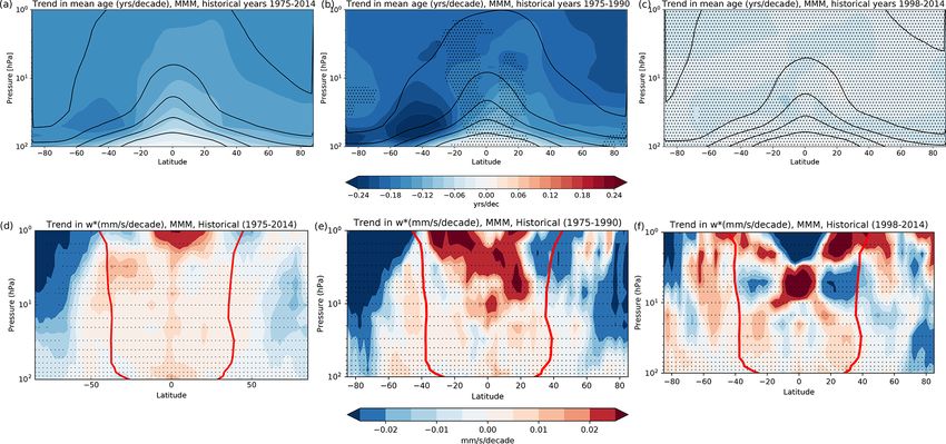
13572                                                                                            M. Abalos et al.: The BDC in CMIP6

Table 1. List of CMIP6 models with Transformed Eulerian Mean (TEM) and/or age of air (AoA) diagnostics used in this study. AoA is only
provided in the historical runs for MRI.

 Model                   Model and data references                                  Levels     Model top              TEM   AoA
 CNRM-ESM2-1             Séférian et al. (2019), Séférian (2018a, b)                   91      78.4 km (∼ 0.01 hPa)   X     X
 CESM2-WACCM             Gettelman et al. (2019), Danabasoglu (2019a, b)               70      0.0000045 hPa          X     X
 MIROC6                  Tatebe et al. (2019), Tatebe and Watanabe (2018a, b)          81      0.004 hPa              X     X
 GFDL-ESM4               Dunne et al. (2020), Krasting et al. (2018a, b)               49      0.01 hPa               X     X
 GISS-E2-2-G             Rind et al. (2020), Orbe et al. (2020), NASA/GISS (2019)     102      0.002 hPa              X     X
 UKESM-1-0-LL            Sellar et al. (2019), Tang et al. (2019a, b)                  85      85 km (∼ 0.005 hPa)    X     X
 HadGEM3-GC31-LL         Williams et al. (2018), Ridley et al. (2019a, b)              85      85 km (∼ 0.005 hPa)    X     X
 MRI-ESM2-0              Yukimoto et al. (2019a, b, c)                                 80      0.01 hPa               X     X(historical)

former approximately limited to latitudes below 50◦ N/S and             as model output (Gerber and Manzini, 2016). This allows for
levels below 50 hPa and overturning timescales under 1 year             a more detailed analysis based on a consistent set of diag-
(Birner and Bönisch, 2011). In the literature, the term BDC             nostics as compared to previous assessments (e.g., Manzini
sometimes refers to the residual circulation alone, and pre-            et al., 2014; Hardiman et al., 2014). Here, we use this TEM
vious multimodel assessments of the BDC focused on this                 and AoA output to evaluate the past climatology and trends in
component (i.e., Butchart et al., 2010; Hardiman et al., 2014).         the BDC against reanalyses and observations using historical
However, there is growing evidence over the last years of the           simulations and to assess the BDC response to an idealized
important role of mixing for net stratospheric tracer transport         1 % yr−1 CO2 increase. In Section 2 we describe the CMIP6
(Garny et al., 2014; Dietmüller et al., 2017; Eichinger et al.,         models and simulations used, as well as other datasets em-
2019; Ploeger et al., 2015). The mean age of air (AoA) trans-           ployed. Section 3 analyzes the BDC in historical simulations,
port diagnostic quantifies the elapsed time since an air parcel         Sect. 4 examines the BDC changes associated with increases
entered the stratosphere, and it can be estimated from obser-           in CO2 , and Sect. 5 explores the connections between BDC
vations of long-lived tracers such as SF6 or CO2 (e.g., Engel           and surface warming. The main conclusions are summarized
et al., 2017). Therefore, it integrates the effect of both resid-       in the last section.
ual circulation and mixing. While there are no direct mea-
surements of the BDC strength, model results can be evalu-
ated against observational estimates of the AoA.                        2    Data and methods
   In this study we assess the climatology and trends in the
                                                                        CMIP6 models providing the necessary TEM and/or AoA
BDC in CMIP6 models, with a focus on current open ques-
                                                                        output, as described in Gerber and Manzini (2016), have been
tions. A key open question is the disagreement between ob-
                                                                        used. We refer to that paper for the specific diagnostic de-
servations and models regarding the past BDC trends. While
                                                                        scription. Table 1 shows the models used, their number of
models consistently predict a reduction in AoA mainly due to
                                                                        levels, the model top and the corresponding available vari-
an acceleration of the residual circulation (Li et al., 2018), the
                                                                        ables. While each model has a different horizontal resolu-
longest observational estimates produce nonsignificant posi-
                                                                        tion (not shown), they are all in the range between 1 and 2◦
tive trends (Engel et al., 2017). Various studies over the last
                                                                        in longitude and latitude. Note that two more models out-
years suggest that an acceleration of the BDC might actu-
                                                                        put TEM variables, CESM2 and Can-ESM5, but we did not
ally be observed in the lower stratosphere (see Karpechko
                                                                        include them in the analyses, because they have low model
et al., 2018, and references therein). Moreover, it has been
                                                                        tops (2.25 and 1 hPa, respectively) and did not represent the
argued that the formation of the ozone hole has had a signif-
                                                                        residual circulation structure adequately (not shown).
icant impact on the past BDC acceleration until the end of
                                                                           Model results have been compared to reanalysis over the
the 20th century (Oman et al., 2009; Li et al., 2018; Polvani
                                                                        historical period. Because there is a large spread in the
et al., 2018; Abalos et al., 2019). However, the observation–
                                                                        residual circulation values obtained from reanalyses (Abalos
model discrepancy remains at higher altitudes. Indeed, the
                                                                        et al., 2015), we used three reanalyses: ERA-Interim (Interim
trends in the deep branch and its drivers remain more uncer-
                                                                        European Centre for Medium-Range Weather Forecasts Re-
tain (WMO, 2018), given the limitations of model top and
                                                                        analysis; Dee et al., 2011), JRA-55 (Japanese 55-year Re-
the importance of parameterized gravity waves in the upper
                                                                        analysis; Kobayashi et al., 2015) and MERRA (Modern-Era
stratosphere and mesosphere. On the other hand, recent work
                                                                        Retrospective analysis for Research and Applications; Rie-
has highlighted that the observational AoA trend estimates
                                                                        necker et al., 2011). We have used the residual circulation for
are likely biased high (Fritsch et al., 2020).
                                                                        these three reanalyses from Abalos et al. (2015), which cov-
   CMIP6 is the first CMIP activity providing Transformed
                                                                        ers the period 1979–2012. In order to compare AoA with ob-
Eulerian Mean (TEM) diagnostics and mean age of air (AoA)
                                                                        servational estimates, we used AoA derived from the Michel-

Atmos. Chem. Phys., 21, 13571–13591, 2021                                                    https://doi.org/10.5194/acp-21-13571-2021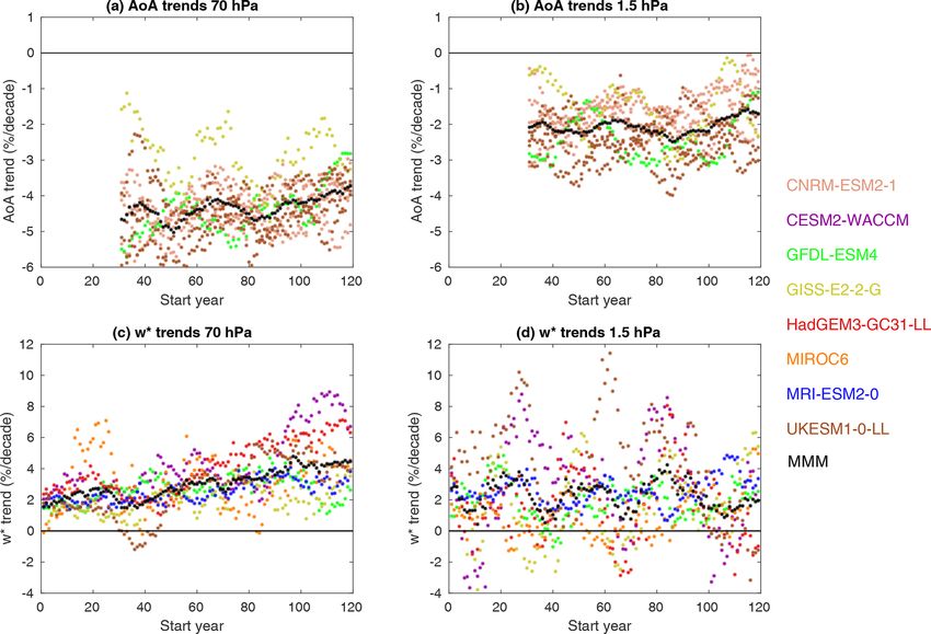
M. Abalos et al.: The BDC in CMIP6                                                                                                    13573

Figure 1. Annual-mean climatology for the multi-reanalysis mean (a) and multimodel mean for the historical simulations (b) of the vertical
component of the residual circulation (w∗ , in mm s−1 , shading) and residual streamfunction (9 ∗ , in kg m−1 s−1 , contours). Black thick
contours indicate the location of the turnaround latitudes. The red contour in the right panel shows the turnaround latitudes for reanalyses.
Black dots represent regions where there is disagreement in the sign of w∗ for more than 66 % (2/3) of the individual reanalyses or models
(which happens only around turnaround latitudes).

son interferometer MIPAS (Stiller et al., 2012; Haenel et al.,           Student t test at the 95 % confidence level. We further ask for
2015). Here, we use a new version of AoA derived from an                 two-thirds (2/3) of the models to agree (that is, 5 out of 7 for
updated retrieval of SF6 (Stiller et al., 2020). Furthermore,            the residual circulation and 4 out of 5 for AoA).
AoA derived from GOZCARDS N2 O data is used (Linz
et al., 2017), as well as AoA data derived from in situ mea-
surements of CO2 and SF6 by Engel et al. (2017) and An-                  3     Representation of the BDC in CMIP6 historical
drews et al. (2001).                                                           simulations
   The model simulations used are historical and 1pctCO2.
                                                                         This section aims to assess the degree of agreement in the
We use one member of each simulation because there is
                                                                         BDC climatology and trends between CMIP6 historical sim-
a very uneven number of members for the different mod-
                                                                         ulations and observations or reanalysis data.
els (from 1 to 18); therefore, the comparison across mod-
els would be unfair if the ensemble mean were used for                   3.1    Climatology and seasonality
each model. Nevertheless, we do exploit the multiple mem-
bers when available in order to explore the role of internal             Figure 1 shows the climatological structure of the residual
variability on the trends (Figs. 5–7 and 10). The fully cou-             circulation in the CMIP6 multimodel mean (MMM, Fig. 1b)
pled (DECK) historical simulations cover the period 1850 to              compared with the multi-reanalysis mean (Fig. 1a). The cli-
2014, with observed emissions of greenhouse gases and other              matological structure and magnitude are overall very similar
external forcings, and they will be used to examine past cli-            in both datasets. Both models and reanalyses highlight a min-
matology and trends and to compare them to observations                  imum in tropical upwelling at ∼ 50 hPa of about 0.2 mm s−1
or reanalysis when possible. For comparison purposes we                  and a maximum at ∼ 1.5–2 hPa of about 1.2 mm s−1 . The
have focused on the period 1975–2014. Note that this period              annual-mean residual circulation structure in Fig. 1 is con-
encompasses the reanalysis period considered (1979–2012),                sistent with previous model intercomparison studies such as
but it is slightly longer. This is done to enhance statistical sig-      CMIP5 (Hardiman et al., 2014).
nificance in trend calculations for model output. The small                 In order to examine the quantitative differences in more
difference in the period considered is assumed to have a neg-            detail, the tropical upwelling mass flux is examined. This
ligible impact on the climatological BDC. The 1pctCO2 sim-               is computed as the net upwelling between the annual-mean
ulations are initialized from preindustrial (1850) conditions            turnaround latitudes (i.e., the latitudes separating the up-
and are 150 years long, with CO2 concentrations increasing               welling and downwelling regions). The calculation is based
gradually at a 1 % yr−1 rate (Eyring et al., 2016). In order             on the streamfunction, which in turn is computed from the
to establish statistical significance, we have used a two-tailed         meridional component of the residual circulation provided

https://doi.org/10.5194/acp-21-13571-2021                                               Atmos. Chem. Phys., 21, 13571–13591, 2021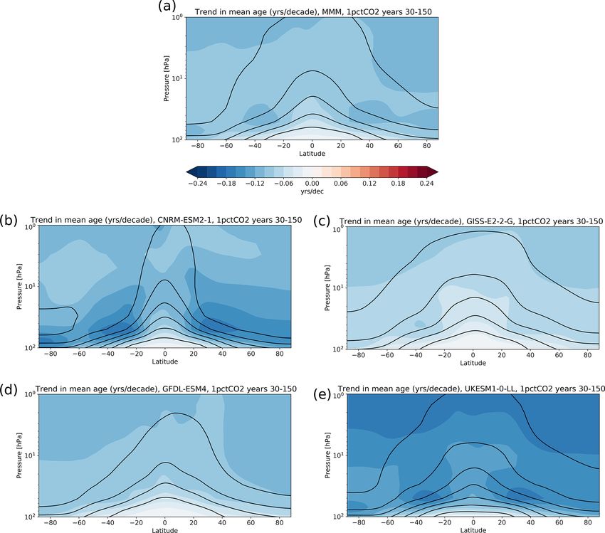
13574 M. Abalos et al.: The BDC in CMIP6
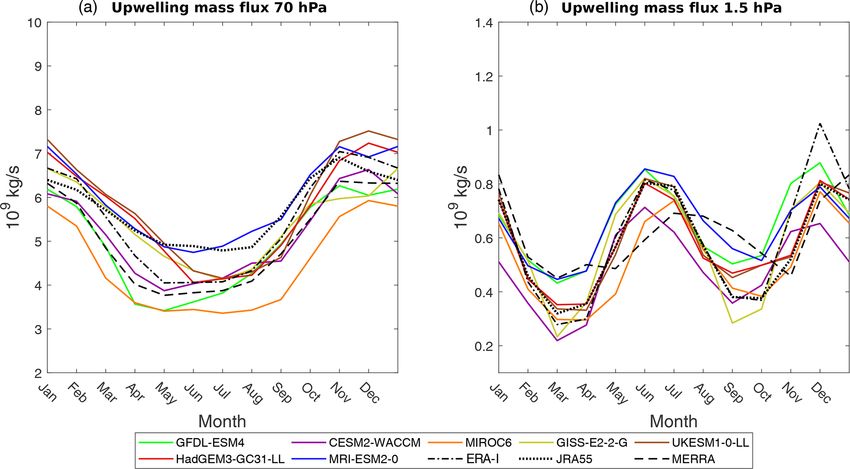
Figure 2. Seasonal cycle of tropical upwelling mass flux in the lower stratosphere (70 hPa, a) and in the upper stratosphere (1.5 hPa, b). Solid
color lines show models, and dashed black lines show reanalyses.
as model output, v ∗ . The streamfunction is obtained as spread is over 40 % of the climatological mean for the lower
stratosphere and over 30 % for the upper stratosphere. The
Z0
∗ cos φ annual cycle in the lower stratosphere has been linked to sea-
9 (φ, p) = − v ∗ dp 0 , (1) sonality of wave forcing in the extratropics, subtropics and
g
p tropics (e.g., Randel et al., 2008; Ueyama et al., 2013; Or-
where p is pressure, φ is latitude, g the gravitational constant tland and Alexander, 2014; Kim et al., 2016). The semian-
on Earth, and it is assumed that v ∗ tends to zero as p → 0. nual cycle in the upper stratosphere has been less studied. It
The upwelling mass flux is then computed at each level as is linked to the combined annual cycles of downwelling in
each hemisphere (which have similar magnitude, in contrast
∗ ∗
M(p) = 2π a 9 max (p) − 9 min (p) , (2) with the lower stratosphere where the Northern Hemisphere
(NH) dominates). In addition, there is likely a contribution
∗ ∗
where 9 max and 9 min are the maximum and minimum val- from the secondary circulation associated with the semian-
ues of the residual streamfunction at each pressure level, nual oscillation (e.g., Garcia et al., 1997; Young et al., 2011),
which correspond to the northern and southern turnaround although this peaks at higher levels (∼ 0.1 hPa; Smith et al.,
latitudes, respectively (Rosenlof, 1995). 2017).
Figure 2 shows the seasonality in the tropical upwelling As mentioned in the Introduction, the mean age of air pro-
mass flux for the lower (70 hPa) and upper (1.5 hPa) strato- vides an estimate of the net transport circulation strength that
sphere, representative of the shallow and deep branches, can be compared to observational estimates. Figure 3 shows
respectively. Note that, while the level of 70 hPa is com- the AoA climatology at 50 hPa for the models that provide
monly used to represent the shallow branch, 1.5 hPa is higher this quantity (see Table 1), together with the observational es-
than usually considered for the deep branch, though it has timates described in Sect. 2. The simulated AoA values show
been used before (Palmeiro et al., 2014). We argue that this considerable spread across models, as previously shown for
level is optimal for the characterization of the deep branch, Chemistry-Climate Model Intercomparison project (CCMI)
since tropical upwelling maximizes at this level in the upper simulations (e.g., Dietmüller et al., 2017). The global mean
stratosphere (Fig. 1). All models show a generally consis- age values vary by a factor of 2, between 2.5 and 5 years
tent seasonality, with an annual cycle peaking in November– approximately. Nevertheless, the spread is within the large
December in the shallow branch, an amplitude of about 50 % observational uncertainty. Note that the relationship between
of the climatological mean, and a semiannual cycle peaking AoA and residual circulation strength is not straightforward.
in June and December for the deep branch, with an ampli- For example, the GFDL model features a weak upwelling,
tude of about 80 %. The seasonality is consistent with that but the AoA is relatively young. In contrast, MRI has strong
of reanalyses, and the intermodel spread is of similar mag- upwelling, but the AoA is the oldest. This lack of corre-
nitude to the reanalysis spread. In particular, the intermodel
Atmos. Chem. Phys., 21, 13571–13591, 2021 https://doi.org/10.5194/acp-21-13571-2021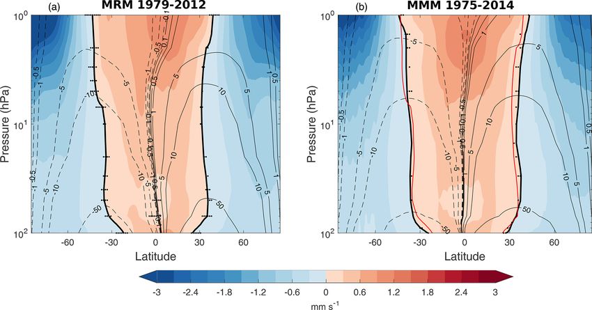
M. Abalos et al.: The BDC in CMIP6                                                                                              13575

                                                                       lower stratosphere larger in the Southern Hemisphere (SH)
                                                                       than in the Northern Hemisphere (NH). Consistently, the
                                                                       residual circulation accelerates throughout the stratosphere,
                                                                       with enhanced tropical upwelling and polar downwelling,
                                                                       strongest in the SH. Note that there is also reduced down-
                                                                       welling in midlatitudes in both hemispheres. The larger po-
                                                                       lar downwelling trends in the SH are consistent with recent
                                                                       results using CCMI models and reflect the contribution of
                                                                       ozone depletion in the Antarctic lower stratosphere to the
                                                                       BDC trends (Polvani et al., 2018, 2019; Abalos et al., 2019).
                                                                       In order to better capture this signal, the trends are shown
                                                                       separately for the end of the 20th century, which is a period
                                                                       of severe ozone depletion (Fig. 4b and e), and the beginning
                                                                       of the 21st century, when ozone depletion stops and its re-
                                                                       covery starts (Fig. 4c and f). It is clear that the BDC trends
                                                                       are stronger during the ozone hole formation, particularly
                                                                       in the SH. The AoA trends for 1975–1990 are significantly
                                                                       different from those for 1998–2014 in the SH lower strato-
Figure 3. Annual-mean AoA at 50 hPa for historical simulations av-
                                                                       sphere and in the NH above 30 hPa and north of about 40◦ N
eraged over 1990–2014, including the standard deviation of the an-
                                                                       (not shown). Note that we have excluded the period 1991–
nual means. Observationally derived AoA values are shown based
on SF6 measurements by MIPAS from 2005–2011 (Stiller et al.,           1997 from the time series in order to avoid the influence of
2020) and N2 O measurements from the GOZCARDS data set for             Pinatubo volcanic eruption on the trends. We caution that the
2004–2012 (Linz et al., 2017). For both, vertical bars represent the   trends are computed over short periods, and the residual cir-
spread between minimum to maximum annual-mean values. In ad-           culation presents high interannual variability, such that there
dition, AoA values are shown as derived from in situ measurements      is no statistical significance of the trends (Fig. 4d–f). Never-
of SF6 and CO2 by Andrews et al. (2001). The error bars for the        theless, the influence of the ozone hole is clearly seen in the
in situ measurements represent uncertainty in the measurement and      different trend magnitudes between the two periods, which
derivation of AoA rather than interannual variability.                 are consistent across models.
                                                                          While Fig. 4 shows the general trend behavior for the mul-
                                                                       timodel mean, it is important to assess the robustness of the
spondence emphasizes the important role of mixing, includ-             trends across different members and models, especially given
ing subgrid effects, in determining the net transport strength         the relatively short periods under consideration. Figure 5 ex-
(Garny et al., 2014; Dietmüller et al., 2017). The tropical            amines the intermodel spread as well as the inter-member
leaky pipe model relates the net upwelling through an isen-            spread for each model, which quantifies the influence of in-
trope with the mass flux-weighted tropics/extratropics gradi-          ternal climate variability on the trends. To do so, a histogram
ent in AoA (e.g., Linz et al., 2016). Linz et al. (2017) revealed      of trends for AoA and tropical upwelling is shown in Fig. 5
a large discrepancy in the overturning circulation strength de-        using all the members of each model. For upwelling, the
rived from the AoA gradient between the WACCM model                    same levels as in Fig. 2 are used in order to separate the
and an older version of MIPAS observations, except at a level          shallow and deep branches. For AoA, the trends are shown
near 20 km. As a note, we applied a simple approximation of            over the regions with available trend estimates from observa-
this method by computing the area-weighted age gradient on             tions, that is, the NH midlatitude lower stratosphere (80 hPa)
pressure levels (not shown) and found a relationship with the          and mid-stratosphere (30 hPa). Observational trend estimates
net upward mass flux for the 1pctCO2 runs (three models)               of AoA are shown for 80 hPa and displayed in the legend
but not for the historical runs (four models). We therefore            for 30 hPa, as they are outside the range of the abscissa. In
cannot extract robust conclusions due to the limited number            addition, the MMM trends from CCMI have been included
of models providing AoA output.                                        in all panels. We do not include reanalysis trend estimates
                                                                       for upwelling, because these show a larger spread than the
3.2   Past trends                                                      models and thus do not help constrain the results (Abalos
                                                                       et al., 2015). In the lower stratosphere there is very good
In this section we examine the BDC trends over the historical          agreement between the CMIP6 MMM AoA trends and the
period, in particular over the last 4 decades. Figure 4 shows          observed trends (Fig. 5a). The trend in the CCMI MMM is
the multimodel mean trends in AoA (Fig. 4a) and vertical               also negative but not as strong. Note, however, the reduced
component of the residual circulation (w ∗ , Fig. 4d) over the         number of models with AoA output in CMIP6. In the mid-
period 1975–2014. The AoA trends are negative everywhere               dle stratosphere (Fig. 5b) the MMM of both intercompari-
with values around −0.1 years per decade, with trends in the           son projects produces a negative mean age trend between

https://doi.org/10.5194/acp-21-13571-2021                                            Atmos. Chem. Phys., 21, 13571–13591, 2021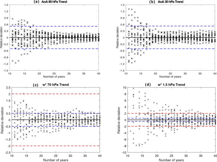
13576                                                                                             M. Abalos et al.: The BDC in CMIP6

Figure 4. Multimodel mean linear trend in AoA (a–c, years per decade) and w∗ (d–f, in mm s−1 per decade) from historical simulations in
shading over years 1975–2014 (a, d) 1975–1990 (b, e) and 1998–2014 (c, f). In the top panels the contours show the climatological AoA
(years, contour interval 1 year, lower contour: 1 year). In the bottom panels the red contours show the turnaround latitudes averaged over
each corresponding period. Stippling indicates statistically insignificant trends obtained with a Student’s t test at 95 % confidence level for
more than 66 % of the models.

−2 % per decade and −3 % per decade, which is stronger                    do not necessarily imply positive AoA trends, because the
for CMIP6. These values disagree strongly with the observed               latter is an integrated quantity, affected non-locally by both
estimate of +3 % per decade, even when taking the large un-               advection and mixing (e.g., Garny et al., 2014; Linz et al.,
certainty into account. Even if one considers the updated es-             2016). Indeed, the GISS and UKESM simulations that pro-
timate of AoA trends by Fritsch et al. (2020) of +1.5 ± 3 %               duce negative upwelling trends (Fig. 5d) still present a de-
per decade, the range of model estimates barely overlaps with             crease in AoA in the middle stratosphere (Fig. 5b). Finally,
the observational uncertainty range. The residual circulation             note that the spread among individual models is comparable
trends in the shallow branch (Fig. 5c) range from 0.5 % per               to the spread between ensemble members of one model both
decade to 3.5 % per decade, with a maximum in the distribu-               for AoA and upwelling and throughout the stratosphere. This
tion slightly below 2 % per decade, consistent with previous              highlights the vital role of internal variability for determining
climate model simulations. The CMIP6 MMM trend is in ex-                  the trends.
cellent agreement with that from the CCMI MMM (Fig. 5c).                     We next examine the role of the limited sampling in the
In the middle stratosphere, the value of the CMIP6 MMM                    observational data on the detection of trends. Figure 6 shows
trend is similar to that in the shallow branch (slightly be-              time series and trends of AoA from the models subsampled
low 2 % per decade), while the trend in the CCMI MMM is                   at the locations and times of the Engel et al. (2009) mea-
weaker (Fig. 5d).                                                         surements (though using monthly-mean zonal mean output
   When looking at individual simulations, the AoA trends                 and averaging over the mean altitude of the measurements,
show a similar spread in the trends across simulations of                 24–35 km). Also included are observational estimates of the
less than 3 % per decade at the two levels. In contrast, the              AoA and its uncertainty from observations, both from Engel
residual circulation trends show a larger spread in the deep              et al. (2009) and from the updated version from Fritsch et al.
branch than in the shallow branch, with some members fea-                 (2020), in which different parameters are used in the deriva-
turing slightly negative trends in the deep-branch upwelling              tion of AoA from the tracer measurements. The latter study
(trends range from almost −1 % per decade to over 5 % per                 showed large sensitivity of AoA trends to assumed parame-
decade). Therefore, a deceleration of the deep branch over                ters in the derivation of AoA from nonlinear increasing trac-
1975–2014 is compatible with the internal variability in some             ers. Here, AoA values derived with optimized parameters are
of the CMIP6 models (although in the tail of the distribu-                shown (using the convolution method and a ratio of moment
tion), which could be consistent with observational AoA es-               of 1.25; for details see Fritsch et al., 2020). The subsampled
timates. Nevertheless, we note that negative upwelling trends             trends are negative for every simulation, contrasting with the

Atmos. Chem. Phys., 21, 13571–13591, 2021                                                   https://doi.org/10.5194/acp-21-13571-2021
M. Abalos et al.: The BDC in CMIP6                                                                                                   13577

Figure 5. Absolute frequency distribution of trends (in % per decade) over 1975–2014 from individual models and ensemble members in AoA
at 80 hPa (a) and 30 hPa (b) averaged over 30–45◦ N and in tropical upwelling at 70 hPa (c) and 1.5 hPa (d). In panel (a) the observational
trend estimate at 80 hPa over 1975–2012 from Ray et al. (2014) updated for the 2018 WMO ozone assessment report (Karpechko et al.,
2018) is included as a black solid line. In panel (b), the observational trend estimate at 30 hPa over 1975–2017 from Engel et al. (2017) is
only shown in the legend, as the value is positive and thus outside the scale. Dashed lines show the MMM for CMIP6 models (black) and
for CCMI models (gray). In panel (c) a colored circle is shown where a bar is covered by another model’s bar. The number of available
members from the historical simulations is 5 for CRNM-ESM2-1, 3 for CESM2-WACCM, 1 for GFDL-ESM4, 4 for GISS-E2-2-G, 4 for
HadGEM3-GC31-LL, 1 for MIROC6, 5 for MRI-ESM2-0-LL, and 18 for UKESM1-0-LL.

positive trends in the observational estimates (Fig. 6b). How-          respect to the ensemble mean, as a function of the length
ever, in this case the model trends are compatible with the             of the period (Fig. 7). The trends of AoA and upwelling are
observational trends from Fritsch et al. (2020) in 14 out of            shown at the same regions as in Fig. 5. The results for AoA in
the 32 simulations (43 %), for which the model and obser-               the NH midlatitudes show that the trends agree within ±30 %
vational trend error bars overlap. It is important to point out         with the ensemble mean for periods longer than ∼ 22 years
that the uncertainties in the subsampled model AoA trends               (Fig. 7a and b). Given that the longest observational AoA es-
are 5 times larger on average than those using all model data,          timates cover more than 30 years, natural variability cannot
going from a 10 % to a 50 % uncertainty on average (not                 explain the discrepancy between the negative trends in the
shown). These large error bars due to subsampling are re-               models and the positive trend in AoA derived from observa-
sponsible for the agreement within uncertainties with obser-            tions in the middle stratosphere. However, this argument as-
vations obtained for some of the model simulations. Finally             sumes that the internal variability is realistically represented
we note that, if only the CO2 measurement locations are con-            in the models, which is not necessarily true. When the same
sidered, the model trends are compatible with zero in most of           analysis is done for the residual circulation (Fig. 7c and d),
the simulations (not shown). This is because the early obser-           the trends need to be computed over longer periods to con-
vations before 1985, which are key to get negative trends in            verge to the ensemble mean trend (more than 30 years), and
the models, are based on SF6 (Fig. 6a).                                 even over 40-year periods the trends in different members
   To explore further the role of internal variability, we ana-         converge only to within ±50 % of the ensemble mean, for
lyze how the trends depend on the length of the period con-             the shallow branch (Fig. 7c), and to within ±200 % in the
sidered. Hardiman et al. (2017) estimated the time of emer-             deep branch (Fig. 7d). At 10 hPa the 40-year trends show a
gence of robust trends in tropical upwelling to be around               ±150 % spread (not shown). These results highlight the sub-
30 years. Here, we consider 18 ensemble members from the                stantially larger internal variability in the deep branch than
UKESM model and compute the departure of the trends with                the shallow branch of the residual circulation and show that

https://doi.org/10.5194/acp-21-13571-2021                                               Atmos. Chem. Phys., 21, 13571–13591, 2021
13578                                                                                       M. Abalos et al.: The BDC in CMIP6

                                                                      sistent with previous results (Palmeiro et al., 2014; Hardi-
                                                                      man et al., 2014). In the upper stratosphere, Hardiman et al.
                                                                      (2014) found a widening of the turnaround latitudes for
                                                                      CMIP5 MMM. They suggested that this change was as-
                                                                      sociated with a strengthening of the polar vortex in both
                                                                      hemispheres, which leads to reduced equatorward refraction
                                                                      of planetary waves. A more modest widening is found in
                                                                      the CMIP6 MMM, limited to the NH, perhaps linked to a
                                                                      strengthening of the polar vortex in the MMM for the sub-
                                                                      set of CMIP6 models used in the present study (not shown).
                                                                      Nevertheless, we note that the trends in the polar vortex are
                                                                      highly model dependent, and for instance the two models
                                                                      that show a clear widening of the tropical pipe in the NH
                                                                      upper stratosphere (CESM-WACCM and HadGEM) feature
                                                                      opposite-sign trends in the polar vortex. On the other hand,
                                                                      more detailed comparisons cannot be made since the forcings
                                                                      are different (RCP8.5 scenario in Hardiman et al., 2014, ver-
                                                                      sus 1pctCO2 here). Despite the overall consistent structure of
                                                                      the trends, there is a notable spread in w∗ trends, especially in
                                                                      the upper stratosphere (above 10 hPa), as will be quantified
                                                                      below. This is consistent with the large spread in the deep-
Figure 6. (a) Time series of AoA (in years) from individual model
simulations sampled at the locations and times of the measurements
                                                                      branch trends in the historical period discussed above. All
from Engel et al. (2009), with different symbols representing the     models show stronger deep-branch downwelling trends in the
SF6 and CO2 measurements. Specifically, the zonal mean AoA has        NH than the SH, and most models even feature slightly posi-
been averaged over the 24–35 km range and evaluated at the lati-      tive trends in the SH polar lower stratosphere. Such asymme-
tude and month corresponding to each measurement. Observational       try is not seen in the downwelling of the shallow branch over
estimates from Engel et al. (2009) and updated after Fritsch et al.   midlatitudes. A weakening of the polar downwelling in the
(2020) are included for comparison. (b) Trends in the time series     SH was also seen in CCMI full-forcing simulations, linked
in (a) for each model member and the observational estimates, with    to ozone hole recovery, which is however not present in the
error bars corresponding to the 95 % confidence level. The trends     1pctCO2 runs. Indeed, this weakening was not observed in
are computed for the combined time series considering both tracers.   CCMI sensitivity simulations in which ozone-depleting sub-
The individual measurement uncertainties are taken into account to
                                                                      stances did not change (Polvani et al., 2018, 2019). On the
calculate the trend error bar.
                                                                      other hand, a weakened downwelling in response to increas-
                                                                      ing CO2 is consistent with an intensification of the SH polar
trends in AoA converge more rapidly to the MMM than those             vortex in response to greenhouse gas increase (McLandress
in upwelling. This is due to the memory of AoA, being an in-          et al., 2010; Ceppi and Shepherd, 2019).
tegrated quantity in both time and space.                                Similar to Fig. 8, Fig. 9 shows the AoA trends in the dif-
                                                                      ferent models and the MMM. The results show a consistent
                                                                      decrease in mean age throughout the stratosphere. In general
4     BDC response to CO2 increase                                    there are weaker trends in the lower stratosphere in the SH
                                                                      than in the NH, consistent with weaker (and even opposite-
In this section we examine the BDC trends and wave forcing            sign) downwelling trends in this hemisphere seen in Fig. 8.
in the 1pctCO2 simulations.                                           There is substantial intermodel spread in the structure and
                                                                      magnitude of the trends. Common features include weaker
4.1    BDC trends                                                     trends in the tropical pipe than at high latitudes and par-
                                                                      ticularly strong trends in the subtropical-midlatitude lower
Figure 8 shows the trend in w ∗ for the 1pctCO2 simula-               stratosphere. The stronger AoA trends in the extratropics as
tions in the different models and for the MMM. This figure            compared to the tropics and associated reduction in age gra-
clearly demonstrates the increasing strength of the residual          dient are consistent with the overturning acceleration, as re-
circulation due to CO2 increase, in both the deep and shal-           vealed by the leaky pipe model (Neu and Plumb, 1999). This
low branches. The trend is particularly strong in the lower           feature has also been linked to changes in mixing and to
stratosphere and near the stratopause, mirroring the clima-           the upward shift of the circulation linked to tropopause rise
tological structure (Fig. 1). Changes in the turnaround lati-         (Oberländer-Hayn et al., 2016; Sacha et al., 2019).
tudes indicate that the upwelling region narrows in the lower            Figure 10 explores the time dependence of AoA and up-
stratosphere in almost all models. These features are con-            welling trends in the 1pctCO2 runs. This is achieved by plot-

Atmos. Chem. Phys., 21, 13571–13591, 2021                                             https://doi.org/10.5194/acp-21-13571-2021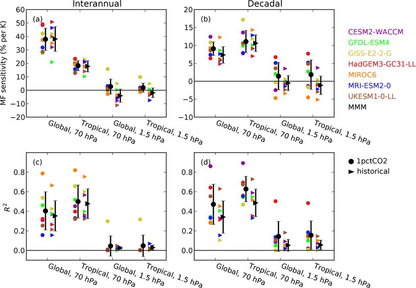
M. Abalos et al.: The BDC in CMIP6                                                                                                13579

Figure 7. Trends from 18 ensemble members of UKESM1-0-LL for periods of increasing length (x axis), ranging from 11 years (1975–
1985) to 40 years (1975–2014). Trends of individual ensemble members (crosses) are displayed as relative deviations from the ensemble
mean trend. Panels (a) and (b) show trends in AoA and panels (c) and (d) show trends in upwelling; both variables are at the same regions
as in Fig. 5. Horizontal dashed lines mark fixed values to ease comparison across panels.

ting trends for moving 30-year periods for each simulation             variability, as shown by the large inter-member spread and by
to find out if trends are approximately constant or if they de-        the strong dependence on the length and starting year of the
pend on the period under consideration. Note that, because             trend period. This contrasts with more stable and less uncer-
there is no comparison with observations, we consider here             tain trends in the shallow branch. They also reveal that AoA
the same regions for AoA and upwelling, representing the               is a less noisy variable, featuring consistently negative trends
shallow and deep branches of the BDC. For individual sim-              in the deep branch across models and members, in contrast
ulations, the trends vary strongly for different periods. These        to the residual circulation.
variations are the largest for tropical upwelling in the deep
branch, with several near-zero and even negative trend peri-           4.2   Drivers of the BDC trends
ods (Fig. 10d). These large oscillations in the deep-branch
upwelling trends are reflected in the MMM. Note that the               Figure 11 shows the contribution of the forcing from dif-
apparent periodicity of about 30 years is an artifact of the           ferent waves to the vertical distribution of the net tropical
30-year period used to compute the trends related with the             upwelling for the MMM. To do so, the downward control
Gibbs ringing (Gibbs, 1898), as we have checked by chang-              principle has been applied between the annual-mean clima-
ing the length of the period (not shown). In contrast, the up-         tological turnaround latitudes (Palmeiro et al., 2014). As a
welling trend in the shallow branch is more consistently pos-          novelty from previous multimodel assessments, here we ex-
itive throughout the period and shows an increase in the trend         amine the entire stratosphere, including the forcing of the
magnitude over time from 2 % per decade to 4 % per decade              deep branch. The CMIP6 MMM results in Fig. 11a show
in the MMM (Fig. 10c). The AoA trends are more similar at              that the climatological behavior of the tropical upwelling
the two levels, with consistent negative values throughout the         is driven fundamentally by resolved waves throughout the
period, despite the large oscillations (Fig. 10a and b).               stratosphere. Their contribution is about 70 % in the shal-
   Figures 5, 7 and 10 demonstrate the high sensitivity of             low branch, peaks in the middle stratosphere reaching 89 %
trends in the deep-branch residual circulation to the internal         near 7 hPa, and is about 80 % in the upper stratosphere. Pa-
                                                                       rameterized orographic gravity waves contribute 18 % to the

https://doi.org/10.5194/acp-21-13571-2021                                             Atmos. Chem. Phys., 21, 13571–13591, 2021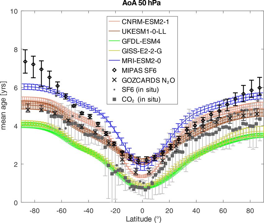
13580                                                                                               M. Abalos et al.: The BDC in CMIP6

Figure 8. Trend in w∗ (mm s−1 per decade), computed using 150-year time series from 1pctCO2 experiments. Panel (a) shows multimodel
mean (MMM). Panels (b) to (h) show individual models. Turn around latitudes show regions of upwelling in the first 20 years (solid red
lines) and last 20 years (dashed red lines) of these 150-year simulations. Stippling in (a) denotes regions where it is not the case that the trend
is significant in at least 66 % of models. Stippling in (b) to (h) denotes regions where the trend in that model is not significant.

Atmos. Chem. Phys., 21, 13571–13591, 2021                                                     https://doi.org/10.5194/acp-21-13571-2021
M. Abalos et al.: The BDC in CMIP6                                                                                                     13581

Figure 9. Multimodel mean linear trend in AoA from 1pctCO2 simulations over years 30–150 in years per decade (shading) and AoA
climatological values averaged over the simulation years 30–60 (black contours, contour interval (ci): 1 year, the lowest contour corresponds
to 1 year). The first 29 years are not considered as the AoA needs time to spin up. Trends are statistically significant everywhere at the 95 %
level for all models.

upwelling at 70hPa, in good agreement with previous mul-                  role in driving trends in the shallow branch. This is due to
timodel studies (i.e., 20 % in CCMVal2 models in Butchart                 the intensification and upward displacement of the subtrop-
et al., 2010), and their contribution decreases at higher alti-           ical jets (not shown) and the upward displacement of the
tudes (6 % at 1.5 hPa). Parameterized non-orographic gravity              critical lines as discussed in other studies (i.e., Garcia and
waves (NOGWs) are not negligible for the shallow branch                   Randel, 2008; McLandress and Shepherd, 2009; Shepherd
and account for about 11 % at 70 hPa, while they become                   and McLandress, 2011; Hardiman et al., 2014). In particu-
the second contributor in the upper stratosphere (15 % at                 lar, at 70 hPa, the contribution to the total trend is 63 % re-
1.5 hPa). Note that model output for NOGWs drag was avail-                solved waves, 25 % OGWs and 11 % NOGWs. In the upper
able only for a small number of models in previous multi-                 stratosphere (above 10 hPa), resolved waves and NOGWs are
model assessments, hampering a direct comparison.                         equally important to the MMM trends, while the contribu-
   As noted above, the vertical structure of the trends in up-            tion from orographic gravity waves is much smaller. This is
welling (Fig. 11b) approximately mirrors that of the climatol-            in agreement with the results of Palmeiro et al. (2014) for
ogy (Fig. 11a). As shown in previous assessments (Butchart                the previous version of WACCM, who explained the key role
et al., 2010; WMO, 2014), resolved waves play the primary                 of NOGW due to changes in the filtering associated with

https://doi.org/10.5194/acp-21-13571-2021                                                 Atmos. Chem. Phys., 21, 13571–13591, 2021
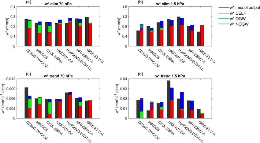
13582                                                                                           M. Abalos et al.: The BDC in CMIP6

Figure 10. Trends in AoA (a, b) and upwelling (c, d) at 70 hPa (a, c) and 1.5 hPa (b, d) calculated from 30-year slices of the 1pctCO2
simulations with start year indicated on the x axis, for each individual simulation (dots; see legend for colors) and the MMM trend (black).
AoA is averaged over 45◦ S–45◦ N and tropical upwelling is averaged between turnaround latitudes. Note that for upwelling only one
member is included, but for AoA all available members are included, in order to have a more comparable total number of simulations for
both variables. The number of available members is 4 for CNRM-ESM2-1, 1 for GFDL-ESM4, 1 for GISS-E2-2-G, and 4 for UKESM1-0-
LL.

changes in the background winds with increasing greenhouse              NOGWs compared to the shallow branch is clear, although
gases. The resolved wave’s contribution peaks approximately             there is quite a range in the contributions of resolved and
at 7 hPa with a 59 % for the MMM. At that level, NOGWs                  NOGWs. Four out of 7 models show comparable contri-
contribute 32 % and OGWs 9 %. At 1.5 hPa the percentages                butions; resolved wave forcing dominates in GISS-E2 and
are 48 %, 41 % and 11 %, respectively.                                  MIROC6, while in CESM2-WACCM there is a comparable
   Figure 12 shows the intermodel spread in wave forcing.               contribution from NOGW and OGW and a negligible con-
The forcing is more consistent across models for the cli-               tribution from resolved waves at 1.5 hPa. These results high-
matology (Fig. 12a and b) than for the trends (Fig. 12c                 light a wide diversity of forcings of the CO2 -driven trends
and d), in agreement with Butchart et al. (2010) results in             among models in the deep branch.
the lower stratosphere (see also WMO, 2014, and references                 Note that there is no proportionality between climatologi-
therein). In the shallow branch, most models (except one)               cal w∗ and its trends across models, in contrast with results
attribute the trends primarily to resolved wave drag. In addi-          from Yoshida et al. (2018) for CMIP5 at 100 hPa. On the
tion, all the models show a relatively small contribution from          other hand, models with larger contributions from gravity
NOGWs (less than 20 %). The contribution from OGWs is                   waves in their climatology tend to have larger contributions
more uncertain: it plays a significant role in four models (be-         in the trends.
ing the main forcing for GFDL-ESM4) but is negligible in
the other three models. Note that a present-day climatolog-
ical source of NOGWs is launched at 70 hPa in the extrat-               5   BDC sensitivity to surface warming on different
ropics in MIROC6 (Watanabe, 2008), which may explain the                    timescales
small contribution to the trends at this level and the negative
contribution in the upper stratosphere.                                 Figure 13a shows the sensitivity of the BDC to surface warm-
   The deep-branch trends feature much larger spread, with a            ing, calculated as the trends in upwelling mass flux (shallow
factor of 4 difference between the smallest trends (MIROC6)             and deep branches), relative to the trends in surface temper-
and the largest trends (UKESM) at 1.5 hPa. The larger role of           ature (global and tropical). The results are shown for histor-

Atmos. Chem. Phys., 21, 13571–13591, 2021                                                 https://doi.org/10.5194/acp-21-13571-2021
M. Abalos et al.: The BDC in CMIP6                                                                                                   13583

Figure 11. Climatology (a) and trends (b) of wave forcing of the residual circulation for the MMM, computed over the 150 years of the
1pctCO2 simulations. Dashed line: tropical upwelling provided as model output; solid black line: total upwelling from downward control
principle (DCP); red line: upwelling due to resolved waves, computed from the Eliassen–Palm flux divergence (DELF); green line: upwelling
due to orographic gravity waves (OGWs); and blue line: upwelling due to non-orographic gravity waves (NOGWs). Note that the GISS model
is not included, because the NOGW output was not available.

Figure 12. Decomposition into forcing from different waves of the tropical upwelling at 70 hPa (a, c) and 1.5 hPa (b, d) for the climatology
(upper panels) and trends (lower panels) for the separate models, computed over the 150 years of the 1pctCO2 simulations. The black bar
shows the upwelling directly from model output. The other colors are as in Fig. 11: red for resolved waves, green for OGWs and blue for
NOGWs. The semitransparent shading in panels (b) and (d) indicates a negative contribution from a forcing, plotted from the top down in the
corresponding color (e.g., NOGW in panel b for CESM2-WACCM). Note that for the GISS model NOGW output is not available, although
these waves are present in the model.

ical and 1pctCO2 simulations. While all models simulate a               that the historical simulation trends are computed over the
strengthening of the residual circulation in both shallow and           period 1960–2014, because this is when the surface warm-
deep branches along with surface warming in response to cli-            ing is clearest. The trends over the period 1850–1959 (not
mate change, only the shallow branch is subject to a tight              shown) show a very large spread across models. The close
control of the global and tropical surface temperature. Note            connection between the residual circulation shallow branch

https://doi.org/10.5194/acp-21-13571-2021                                               Atmos. Chem. Phys., 21, 13571–13591, 2021
13584                                                                                           M. Abalos et al.: The BDC in CMIP6

Figure 13. (a) Connections between long-term trends in mass flux in the shallow (70 hPa) and deep (1.5 hPa) branches and global and tropical
mean surface temperature. The linear trends for the historical runs are calculated over the period 1960–2014 (triangles); for 1pctCO2 runs,
trends are calculated over years 1–150 (circles). Black error bars show the MMM and 1 standard deviation among models. (b, c) Scatter plots
of trends in mass flux at 70 hPa (b) and 1.5 hPa (c) versus tropical surface warming. The coefficient of determination R 2 across the models
is shown in (b) and (c).

and surface temperature is most evident in the last decades of          pendent of surface temperature; therefore, it reduces further
the historical as well as in the 1pctCO2 simulations. The in-           the – already weak – connection between deep-branch trends
termodel spread in the regression values reflects differences           and surface warming. Note that the behavior is very simi-
in the BDC sensitivity to surface warming among the mod-                lar when the global or the tropical mean surface temperature
els. For the shallow branch, the model sensitivity varies in            trends are considered. The disconnection between the deep
the range from 5 % to 13 % per degree of surface warm-                  branch of the residual circulation and surface temperature is
ing. The strong connection between the shallow branch of                consistent with the study by Chrysanthou et al. (2020), which
the BDC and tropical surface temperature is consistent with             finds that the acceleration of the deep branch is largely due
the findings from previous work (Lin et al., 2015; Chrysan-             to the direct CO2 radiative effect.
thou et al., 2020; Orbe et al., 2020). This statistical relation-          Figure 13b and c further demonstrate the connection be-
ship reflects an underlying dynamical mechanism: tropical               tween (tropical) surface temperature and lower branch trends
surface warming leads to tropical upper tropospheric warm-              (Fig. 13b), as well as the absence of such connection for the
ing, which modifies meridional temperature gradients and                deep branch (Fig. 13c). Specifically, there is a strong cor-
thus wind shear (e.g., Garcia and Randel, 2008), altering the           relation across the model simulations between the shallow-
wave propagation and dissipation conditions (Shepherd and               branch and surface temperature trends (R 2 = 0.69) and a
McLandress, 2011).                                                      much reduced correlation for the deep branch (R 2 = 0.12).
   In contrast, the deep-branch sensitivity to surface temper-          However, note that the high correlation disappears if only
ature is near zero in the historical runs, while in the 1pctCO2         the historical simulations are considered. This is because the
runs it is small but consistently positive across the models            connection is mediated by the upper tropospheric warming,
(Fig. 13a). This difference between the two simulation types            and there is substantial intermodel spread in the ratio of sur-
is likely due to the contribution of ozone depletion to the             face to upper tropospheric warming (see, e.g., Po-Chedley
deep-branch trends in the historical run, shown in Fig. 4. The          and Fu, 2012). This spread only affects the historical simula-
impact of ozone depletion on the residual circulation (present          tions, as they have smaller warming trends than the 1pctCO2
in the historical but not in the 1pctCO2 simulations) is inde-

Atmos. Chem. Phys., 21, 13571–13591, 2021                                                 https://doi.org/10.5194/acp-21-13571-2021
M. Abalos et al.: The BDC in CMIP6                                                                                          13585

simulations. The results in Fig. 13b and c are qualitatively      In contrast, consistent with previous studies, there remains
similar for the global surface temperature trends (not shown).    a clear disagreement in the AoA trends between models and
   The connection between surface temperature and BDC             observations in the middle and upper stratosphere, with mod-
residual circulation is explored at interannual and decadal       els featuring robust negative trends. Even when the model’s
timescales in Fig. 14. The decadal regression coefficients        AoA is subsampled in space and time as the observations, the
(Fig. 14b) show a very high consistency with the trend be-        model trends remain negative in the middle stratosphere for
havior in Fig. 13, both qualitative and quantitative. The cor-    all available models and ensemble members (Fig. 6). Nev-
responding coefficients of determination (R 2 , Fig. 14d) re-     ertheless, in this case a substantial fraction (over 40 %) of
veal that the fraction of variance of the shallow-branch tropi-   the available simulations the model and observed error bars
cal upwelling explained by the surface temperature is around      overlap with the observational estimate updated in Fritsch
35 %–60 %, with a wide intermodel spread (ranging from            et al. (2020). It is important to note that, in addition to the
15 % to 85 %). These values are about 15 % higher for the         sampling, another caveat in the comparison between obser-
1pctCO2 than for the historical simulations and also for the      vational and model AoA data is the differences in the prop-
tropical than for the global surface temperature.                 erties of idealized versus realistic tracers, as discussed in de-
   The explained variances (R 2 ) for interannual variations      tail by Garcia et al. (2011). The trends in the deep branch
show similar values to the decadal timescales and are com-        of the residual circulation reveal a large spread among mod-
parable for the tropical as for the global surface tempera-       els and across different members of the same model (Figs. 5
ture. This implies that the surface warming signal on the         and 7). In particular, the inter-member spread in deep-branch
lower branch of the residual circulation is controlled primar-    residual circulation trends is about ±200 % of the ensem-
ily by tropical temperature. However, the regression values       ble mean trends, even when considering long (40-year) peri-
for the shallow branch are notably higher (approximately          ods. In contrast, for the shallow branch the spread is 4 times
twice as large) for global than for tropical surface temper-      smaller. This reveals a notably stronger influence of inter-
atures (Fig. 14a) in the case of interannual variability. This    nal variability on the deep branch than the shallow-branch
likely reflects the fact that interannual temperature varia-      trends. Importantly, the trends are more robust for AoA than
tions often have an antisymmetric pattern between the tropics     for upwelling, with inter-member spread in the trends below
and extratropics. In particular, the connection between the       ±30 % for periods slightly longer than 20 years, both in the
residual circulation and surface temperature on interannual       lower and middle stratosphere.
timescales is dominated by El Niño–Southern Oscillation              The sensitivity of the BDC to CO2 increase is exam-
(ENSO) (e.g., Calvo et al., 2010), which features strong sea      ined, and the robustness of the trends and their wave forc-
surface temperature (SST) anomalies confined to the tropics       ing are explored. In contrast with previous BDC analyses
and opposite sign anomalies in the extratropics. The globally     based on multimodel assessments with CCMVal, CMIP5 and
averaged surface temperatures attenuate the signal (associ-       CCMI, we focus here on the response to CO2 alone, using the
ated with ENSO) that is mainly responsible for interannual        1pctCO2 simulations. All models produce stronger residual
variability in the mass flux. This results in higher regression   circulation acceleration in the NH than in the SH, and it actu-
coefficients for the global temperature. In contrast, long-term   ally decelerates in the SH polar lower stratosphere, possibly
trends and low-frequency variability have a more uniform          due to the CO2 effects on the polar vortex discussed in recent
latitudinal pattern.                                              work (e.g., Ceppi and Shepherd, 2019). An analysis of the
                                                                  wave forcing of the residual circulation shows that shallow-
                                                                  branch forcing of climatology and trends is mainly due to
6   Conclusions and outlook                                       resolved waves with a contribution from OGWs, consistent
                                                                  with previous studies. For the deep branch, the main drivers
The present paper examines the BDC in CMIP6 models, fo-           of climatology and trends are resolved waves and parameter-
cusing on the residual circulation and the mean age of air.       ized NOGWs, but there is a wide spread across models, espe-
   First, historical simulations are used to compare the cli-     cially for the trends. There is a very large inter-model spread
matology and past trends to observations and reanalyses. The      in deep-branch trends (a factor of 4), which could be linked to
climatological average and seasonality of the BDC in CMIP6        the spread in parameterized gravity wave forcing. In contrast,
models lie within the spread of observational (and reanaly-       the spread in the shallow-branch trends is less than 30 %. The
sis) estimates. However, there is a large spread in the mag-      uncertainty in deep-branch residual circulation trends is em-
nitude among models, which is as large as that across ob-         phasized in the large multidecadal fluctuations found over the
servational estimates. The BDC trends in historical simula-       150 simulation years. On the other hand, the shallow-branch
tions are stronger during the ozone depletion period than af-     trends are found to increase over time with CO2 increase, by
ter, which reflects the important contribution of ozone de-       approximately a factor of 2 for the MMM. In contrast, the
pletion to BDC acceleration shown in previous chemistry-          AoA trends are more robust over time, consistent with the
climate model studies. There is very good agreement be-           results for the historical simulations.
tween models and observations in the shallow-branch trends.

https://doi.org/10.5194/acp-21-13571-2021                                       Atmos. Chem. Phys., 21, 13571–13591, 2021
13586 M. Abalos et al.: The BDC in CMIP6 Figure 14. Regression (a, b) and determination (c, d) coefficients between mass flux in the upper and lower stratosphere with global and tropical mean surface temperature on interannual (a, c) and decadal (b, d) timescales. Interannual variability is obtained as the annual mean minus 5-year running mean data; decadal variability is the detrended 5-year mean. Black error bars show the MMM and 1 standard deviation among models. Triangles denote output from historical runs and circles from 1pctCO2 runs. Finally, the connection between surface temperature and for the MMM of the CMIP6 model subset used in this study, the BDC is investigated. We find a strong connection be- but there is a large spread in the trends in the NH, with some tween the shallow branch of the residual circulation and the models featuring deceleration (not shown). This is consis- tropical and global surface temperature. Long-term trends in tent with large differences in resolved versus NOGW forcing lower stratospheric upwelling feature a sensitivity of 7 %– contributions to the deep branch among models. However, 10% per degree of surface warming in the models (Fig. 13). the compensation mechanism (Cohen et al., 2013; Sigmond On interannual and decadal timescales, surface temperature and Shepherd, 2014) implies that the different relative con- explains 35 %–60 % of the shallow-branch variance on av- tributions from resolved versus parameterized gravity waves erage (Fig. 14). Note that the strong connection of shallow- do not necessarily lead to differences in the net residual cir- branch acceleration with surface warming is consistent with culation trends. Overall, open questions remain regarding the the correlation with the upward shift of the tropopause deep-branch trends and their forcing mechanisms. Reducing pointed out by Oberländer-Hayn et al. (2016). In contrast, the uncertainties in deep-branch trends is particularly relevant to deep-branch variability is not correlated with surface temper- better constrain the future distribution of ozone in the po- ature on any timescale. lar stratosphere, affected not only by direct transport but also One of the key results of the present paper is the difference by the descent of ozone-depleting chemical compounds from between shallow and deep branches of the residual circula- the mesosphere (Maliniemi et al., 2020). tion. The CMIP6 models confirm that, while trends in the The results show that AoA is a much less noisy variable shallow branch can now be reconciled with observations (Fu than w∗ , implying that robust trends could be extracted from et al., 2015; WMO, 2018), much larger uncertainties remain relatively short periods (20 years). The advective circulation for the trends in the deep branch. We note that, while a ro- can be approximated from AoA using the leaky pipe model, bust mechanism for the acceleration for the shallow branch in order to compare with observations, as done in Linz et al. has been described (Shepherd and McLandress, 2011), the (2017). Unfortunately, the global AoA observational esti- drivers of deep-branch acceleration remain largely unex- mates available are not long enough to evaluate trends. In plored. Previous studies point to the effects of stratospheric addition, it is crucial to account for the large uncertainties zonal wind trends on the filtering of NOGWs. The CMIP6 in deriving AoA trends from realistic tracers (Fritsch et al., model results in the present paper confirm the important role 2020). We note that, for the few models providing both AoA of NOGW for the deep-branch trends. The zonal-mean wind and w∗ (three models for 1pctCO2 and four for historical trends show acceleration of the polar jet in both hemispheres simulations), it is not possible to extract robust conclusions Atmos. Chem. Phys., 21, 13571–13591, 2021 https://doi.org/10.5194/acp-21-13571-2021
You can also read