The life cycle of upper-level troughs and ridges: a novel detection method, climatologies and Lagrangian characteristics - WCD
←
→
Page content transcription
If your browser does not render page correctly, please read the page content below
Weather Clim. Dynam., 1, 459–479, 2020
https://doi.org/10.5194/wcd-1-459-2020
© Author(s) 2020. This work is distributed under
the Creative Commons Attribution 4.0 License.

The life cycle of upper-level troughs and ridges: a novel detection
method, climatologies and Lagrangian characteristics
Sebastian Schemm, Stefan Rüdisühli, and Michael Sprenger
Institute for Atmospheric and Climate Science, ETH Zurich, Zurich, Switzerland

Correspondence: Sebastian Schemm (sebastian.schemm@env.ethz.ch)

Received: 12 March 2020 – Discussion started: 3 April 2020
Revised: 4 August 2020 – Accepted: 26 August 2020 – Published: 10 September 2020

Abstract. A novel method is introduced to identify and track      diagnostics such as E vectors. During La Niña, the situa-
the life cycle of upper-level troughs and ridges. The aim is      tion is essentially reversed. The orientation of troughs and
to close the existing gap between methods that detect the         ridges also depends on the jet position. For example, dur-
initiation phase of upper-level Rossby wave development           ing midwinter over the Pacific, when the subtropical jet is
and methods that detect Rossby wave breaking and decay-           strongest and located farthest equatorward, cyclonically ori-
ing waves. The presented method quantifies the horizontal         ented troughs and ridges dominate the climatology. Finally,
trough and ridge orientation and identifies the correspond-       the identified troughs and ridges are used as starting points
ing trough and ridge axes. These allow us to study the dy-        for 24 h backward parcel trajectories, and a discussion of the
namics of pre- and post-trough–ridge regions separately. The      distribution of pressure, potential temperature and potential
method is based on the curvature of the geopotential height       vorticity changes along the trajectories is provided to give in-
at a given isobaric surface and is computationally efficient.     sight into the three-dimensional nature of troughs and ridges.
Spatiotemporal tracking allows us to quantify the maturity
of troughs and ridges and could also be used to study the
temporal evolution of the trough or ridge orientation. First,
the algorithm is introduced in detail, and several illustrative   1   Introduction
applications – such as a downstream development from the
North Atlantic into the Mediterranean – and seasonal cli-         Troughs and ridges are ubiquitous flow features in the upper
matologies are discussed. For example, the climatological         troposphere and are centerpieces of weather and climate re-
trough and ridge orientations reveal strong zonal and merid-      search for good reason. In general, a trough is associated with
ional asymmetry: over land, most troughs and ridges are an-       cyclonic flow and moving cold air equatorward. It is depicted
ticyclonically oriented, while they are cyclonically oriented     as a region of reduced geopotential height on an isobaric
over the main oceanic storm tracks; the cyclonic orientation      surface or enhanced potential vorticity on an isentropic sur-
increases toward the poles, while the anticyclonic orientation    face. The counterpart of a trough is a ridge, which is associ-
increases toward the Equator. Trough detection frequencies        ated with warm air moving poleward, increased geopotential
are climatologically high downstream of the Rocky Moun-           height – corresponding to reduced potential vorticity (PV)
tains and over East Asia and eastern Europe but are remark-       – and anticyclonic flow. Jointly, a trough and a ridge form
ably low downstream of Greenland. Furthermore, the detec-         the positive and negative phases, respectively, of large-scale
tion frequencies of troughs are high at the end of the North      Rossby wave patterns, which shape weather development in
Pacific storm track and at the end of the North Atlantic storm    the midlatitudes. At the equatorial tip of a trough, where
track over the British Isles. During El Niño-affected winters,    the geopotential isolines are closely aligned, a jet streak can
troughs and ridges exhibit an anomalously strong cyclonic         form, and the conservation of the absolute vorticity and a re-
tilt over North America and the North Atlantic, in agreement      gion of diffluent flow predict forced upward motion in the
with previous findings based on traditional variance-based        jet exit region. It is therefore not too surprising that surface
                                                                  cyclogenesis (Petterssen and Smebye, 1971; Sanders, 1988;

Published by Copernicus Publications on behalf of the European Geosciences Union.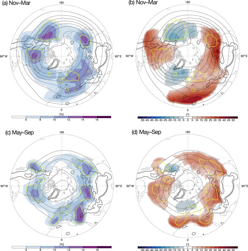
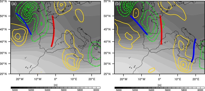
460                                                               S. Schemm et al.: Life cycle of upper-level troughs and ridges

Lackmann et al., 1997; Graf et al., 2017), rapid cyclone in-          associated with a sharpening of the PV gradient along the
tensification (Sanders and Gyakum, 1980; Wash et al., 1988;           edge of the WCB outflow, which corresponds to an accel-
Uccellini, 1990; Wernli et al., 2002; Gray and Dacre, 2006)           eration of the jet. From a momentum flux perspective, the
and enhanced precipitation (Martius et al., 2006; Massacand           center of the WCB outflow corresponds to a region of en-
et al., 2001; Martius et al., 2013) usually take place in the         hanced horizontal eddy momentum flux divergence (leading
region ahead of the upper-level trough axis.                          to a deceleration), and the edge of the WCB outflow corre-
   The shape and orientation of troughs and ridges is pivotal         sponds to a region of enhanced eddy momentum flux con-
in determining their influence on synoptic-scale flow evo-            vergence (leading to an acceleration) (Schemm, 2013). The
lution. A trough or a ridge tilts cyclonically if it forms un-        WCB outflow ahead of an upper-level trough has thus been
der cyclonic shear, while it acquires an anticyclonic orienta-        shown to accelerate downstream cyclone growth (Wernli and
tion if it forms under anticyclonic shear (Davies et al., 1991;       Davies, 1997; Pomroy and Thorpe, 2000; Grams et al., 2011;
Thorncroft et al., 1993). In the case of a pronounced equator-        Schemm et al., 2013) and can even lead to the formation of
ward (poleward) excursion of a trough (ridge), it may wrap            large-scale blocks (Pfahl et al., 2015; Steinfeld and Pfahl,
up and undergo irreversible deformation in a wave-breaking            2019). Recent studies have presented further evidence for the
event (McIntyre and Palmer, 1983; Thorncroft et al., 1993).           non-negligible role of turbulence and radiation in the diabatic
Under anticyclonic shear, the trough deforms into a narrow            modification of the life cycle of troughs and ridges (Spre-
band, called a streamer, which crosses the jet and extends            itzer et al., 2019). The dynamics of troughs and ridges thus
equatorward of the mean jet position and cut-off formation            may act as a stepping stone toward a better understanding of
may occur. During the associated wave-breaking event, the             the coupling between adiabatic and diabatic processes and
jet is pushed poleward. With cyclonic shear, wave breaking            allows for the connection of atmospheric processes from the
occurs poleward of the mean jet position, thereby pushing             planetary scale to the mesoscale.
the jet equatorward (Thorncroft et al., 1993; Lee and Feld-              In this study, a novel feature-based method is introduced
stein, 1996; Orlanski, 2003). The notion of cyclonically and          for identifying and tracking the life cycle of upper-level
anticyclonically oriented wave development is schematically           troughs and ridges, including their axes and orientations, in
summarized in Fig. 12 in Thorncroft et al. (1993). This pro-          gridded data. Feature-based methods for detecting streamers
cess, through which cyclonically or anticyclonically break-           (Wernli and Sprenger, 2007), Rossby wave initiation (Röth-
ing troughs and ridges displace the jet, is even able to excite       lisberger et al., 2016), and wave-breaking events (e.g., Pos-
positive or negative North Atlantic Oscillation events (Bene-         tel and Hitchman, 1999) are widely used research tools, and
dict et al., 2004; Franzke et al., 2004; Rivière and Orlanski,        the motivation behind this work is to extend the capability
2007). A traditional means for quantifying the influence of           of available tools and to track and characterize the entire life
upper-level troughs and ridges on the jet strength and loca-          cycle of upper-level troughs and ridges from genesis to lysis.
tion is the E vector (Hoskins et al., 1983; Trenberth, 1986).         We further aim to compare the detected life cycle character-
With anticyclonic shear, troughs and ridges acquire an anti-          istics of, for example, the trough orientation with previous
cyclonic orientation, and the E vector points equatorward,            results obtained from more traditional methods such as the
indicating poleward eddy momentum flux. With cyclonic                 aforementioned E vectors, thereby bridging gaps between
shear, a poleward-pointing E vector indicates southeast-to-           different perspectives on synoptic-scale evolution.
northwest-oriented troughs and ridges, which correspond to               The trough and ridge detection is used to derive winter
a cyclonic orientation, and the corresponding equatorward             and summer climatologies of their frequency and orienta-
eddy momentum flux pushes the jet equatorward (Hoskins                tion. Further, we address two research questions discussed
et al., 1983; Rivière et al., 2003).                                  in the recent literature. The first concerns the change in the
   Troughs and ridges actively interact with diabatic pro-            orientation of downstream propagating eddies during winters
cesses and are far from being dry adiabatic flow features.            affected by the El Niño–Southern Oscillation (ENSO): dur-
Ahead of the trough axis, where upward vertical motion                ing La Niña, eddies are assumed to acquire a more anticy-
prevails, air from the surface warm sector of a cyclone is            clonic orientation over North America, while they acquire a
lifted within the warm conveyor belt (WCB) to upper lev-              more cyclonic orientation during El Niño (Li and Lau, 2012a,
els (Harrold, 1973; Browning, 1986, 1990; Wernli, 1997).              b; Drouard et al., 2015). Previous studies used the E vector
During ascent, the air is diabatically modified – for exam-           (Hoskins et al., 1983; Trenberth, 1986) to study the eddy ori-
ple by condensation – in a way that amplifies the upper-level         entation. Here, we quantify the trough and ridge tilt using
ridge and the anticyclonic flow downstream of the surface             the automated algorithm. The second research question con-
cyclone (Stoelinga, 1996; Wernli and Davies, 1997; Grams              cerns the midwinter suppression of the North Pacific storm
et al., 2011; Schemm et al., 2013). This process also am-             track: during midwinter, the potential for cyclone growth is
plifies the streamer formation (Massacand et al., 2001) and           largest, but – in contrast to the North Atlantic – the observed
accelerates the jet. From a PV perspective, this phenomenon           storm track intensity over the Pacific is lower compared to the
is seen as a negative PV anomaly around the WCB outflow,              shoulder seasons (e.g., Nakamura, 1992). Using the trough
corresponding to enhanced anticyclonic circulation. It is also        and ridge detection, we explore potential changes in the ori-

Weather Clim. Dynam., 1, 459–479, 2020                                                    https://doi.org/10.5194/wcd-1-459-2020

S. Schemm et al.: Life cycle of upper-level troughs and ridges 461
entation of troughs and ridges because a stronger cyclonic 2.1 Trough and ridge identification
orientation is typically associated with more intense cyclones
(e.g., Fig. 4 in Thorncroft et al., 1993). More detailed liter- The identification of troughs and ridges starts with the geopo-
ature overviews are presented in the corresponding sections. tential height at, for example, 500 hPa, as seen in Fig. 1a for
Finally, we explore the possibility of using the trough and 12:00 UTC on 12 January 2010. Two distinct troughs and one
ridge objects as starting regions for air parcel trajectories in ridge can visually be identified: a northwest-to-southeast-
an effort to explore the diabatic modification of the life cycle oriented trough over the eastern North Atlantic, which is as-
of troughs and ridges. sociated with a mature low pressure system to the west of
The paper is organized as follows. Details of the algorithm Ireland; a meridionally oriented ridge, which extends from
and a case study are presented in Sect. 2. Section 3 is dedi- the Iberian Peninsula to the British Isles; and a meridion-
cated to the discussion of winter and summer climatologies ally oriented trough over the Central Mediterranean to the
and the change in the trough and ridge orientation during southeast of Italy over the Ionian Sea. The goal of an object-
ENSO-affected winters and over the Pacific in midwinter. In based trough and ridge detection is to automatically iden-
Sect. 4, we explore troughs and ridges from a Lagrangian tify these features and the corresponding axes. Several as-
viewpoint before concluding the paper in Sect. 5. pects have to be kept in mind. First, the smooth geopoten-
tial isolines shown in Fig. 1a do not reflect the underlying
1◦ × 1◦ ERA-Interim grid but are already smoothed due to
2 Data and methods the contour-drawing algorithm. Therefore, in the following
panels (Fig. 1b to f), the geopotential height is shown on
The trough and ridge identification algorithm uses 6-hourly the underlying input grid. Second, troughs and ridges may
ERA-Interim data (Dee et al., 2011) but can easily be ap- exhibit a complicated structure. For instance, the horizontal
plied to other gridded data sets. The reanalysis data are orientation can vary along a trough or ridge axis, a trough or
provided publicly by the European Centre for Mid-Range ridge can be broken into different segments, and the curva-
Weather Forecasts (ECMWF) via the following URL: https: ture of the geopotential isolines can considerably vary over
//apps.ecmwf.int/datasets/ (last access: 1 September 2020). small distances. The challenge for an automatic detection al-
More specifically, the identification is demonstrated on the gorithm is to identify all these different characteristics. In the
500 hPa geopotential height data, which are interpolated onto following, details of the proposed algorithm are described.
a regular 1◦ × 1◦ grid. Results based on the 300 hPa geopo- We suggest identifying troughs and ridges geometrically
tential height data are shown in the Supplement. The 500 hPa using the curvature of the geopotential isolines. To this end,
geopotential height has traditionally been used for analy- the change of the orientation of a vector pointing along an
sis of troughs and ridges and continues to be used for re- isoline is computed. First, at every grid point, the gradient
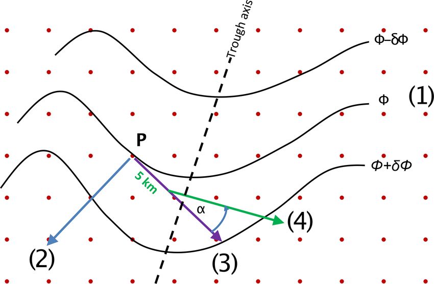
search and forecasting purposes. The presented method is, of the geopotential field is calculated and the gradient vec-
in general, also applicable to different levels or variables, tor is rotated by 90◦ , such that the rotated vector aligns with
e.g., 300 hPa geopotential height, isentropic PV or potential the geopotential isolines. Next, a new location 5 km in the
temperature on the dynamical tropopause. Depending on the direction of the aligned vector is determined, and the cor-
exact research question, the most suitable level and variable responding aligned vector at this new location is obtained
can be chosen. The investigation period is 1979–2018, and trough bilinear interpolation. Because of the curvature of the
the monthly mean trough and ridge climatologies are pub- geopotential isolines, the original vectors and those shifted
licly available (http://eraiclim.ethz.ch/, last access: 1 Septem- by 5 km are rotated against each other, and it is the angle
ber 2020; Sprenger et al., 2017). between these two vectors – normalized by the distance of
This section describes in detail how the trough and ridge 5 km – that we define as the local curvature. The curvature
axes are identified and tracked. Three distinct steps are in- field α(x, y) is available on the whole global grid and is used
volved: to identify the trough and ridge objects. These steps are sum-
marized in Fig. 2.
– identifying 2D trough and ridge objects (masks) and To identify troughs and ridges, a threshold of 0.05◦ km−1
their corresponding axes, is used to mask the curvature field (Fig. 1b). This threshold is
the main degree of freedom of the algorithm. All connected
– tracking the trough and ridge objects and quantifying points in the masked field, which form a coherent object, are
their age and overall lifetimes, clustered into one distinct 2D trough or ridge depending on
the sign of the curvature field (Fig. 1c). Grid points outside
– characterizing the horizontal orientation of each trough a coherent object are flagged with zeros, and grid points in-
and ridge axis. side are marked with ones. Time-averaging over the obtained
binary fields yields detection frequencies, which indicate the
The following subsections will address specific aspects of the fraction of time steps affected by a trough or ridge relative
algorithm, including a detailed validation. to all time steps. We selectively disregard very small features
https://doi.org/10.5194/wcd-1-459-2020 Weather Clim. Dynam., 1, 459–479, 2020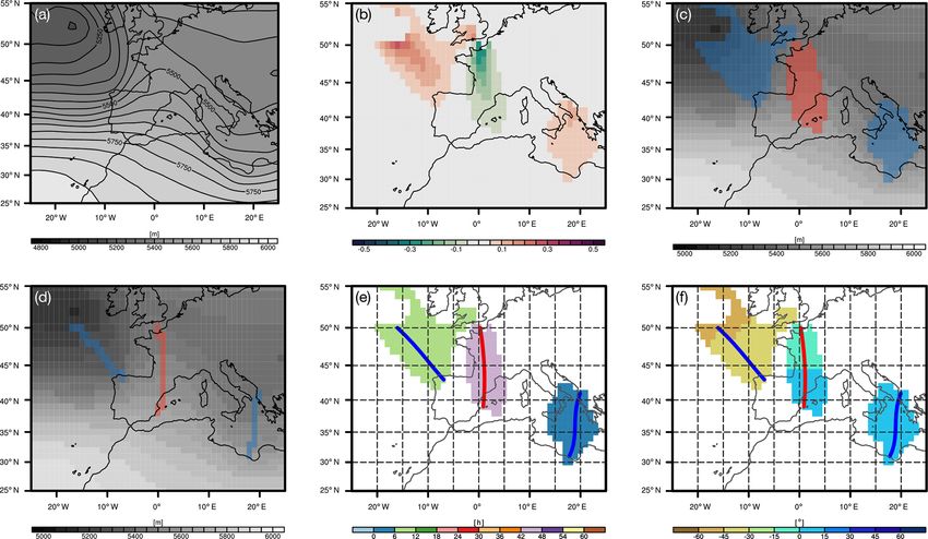
462                                                                   S. Schemm et al.: Life cycle of upper-level troughs and ridges

Figure 1. (a) The 500 hPa geopotential height (m) at 12:00 UTC on 12 January 2010. (b) Curvature of the geopotential isolines (units:
◦ km−1 ) on the 1◦ × 1◦ input grid at every grid point where the curvature is larger than 0.05◦ km−1 . (c) The 2D trough (blue) and ridge (red)
masks and geopotential height (gray shading) at every grid point. (d) The corresponding trough (blue) and ridge (red) axes, (e) Cubic-spline
interpolated trough and ridge axes and age (color; in h) of the trough and ridge features. (f) The horizontal orientation of the trough and ridge
object (in degrees; angle relative to a north–south meridian and estimated from the corresponding axis).

(< 20 × [111 km]2 ), which at this stage are unlikely to corre-               In a final step, the corresponding trough and ridge axes
spond to a significant flow deviation. Additionally, consider-             are identified. The result of this step is shown in Fig. 1d.
ation is only given to midlatitude troughs and ridges within               Algorithmically, a starting point is first selected within each
20–70◦ N, but the algorithm in general could be applied also               2D trough and ridge object; we decided to start at the high-
to polar latitudes. Figure 1 illustrates the individual steps in           est (for troughs) and lowest (for ridges) geopotential value
more details. Figure 1b shows the trough and ridge objects                 within each object. From this starting point, a line is itera-
after masking the normalized curvature field using the above               tively constructed by stepping 5 km forward parallel to the
threshold. The trough over the eastern North Atlantic is con-              geopotential gradient. The iterative extension of the axis line
nected to a mature low-pressure system, which is discernible               ends as soon as it leaves the 2D trough or ridge object. If the
from the closed 500 hPa isolines in the upper-left corner of               identified axis is shorter than 500 km, the axis and the corre-
Fig. 1a and which is also well-marked at the surface. This                 sponding 2D trough or ridge object are removed. This mini-
trough is classified as a “closed trough”. On the other hand,              mum length is the second degree of freedom in our algorithm
the trough object over the Central Mediterranean is not asso-              that the user can adjust. The final outcome of the trough and
ciated with a low-pressure system and is therefore classified              ridge identification is therefore a gridded field, correspond-
by the algorithm as an “open trough”. We decided to classify               ing to the original input grid, on which trough and ridge grid
regions inside closed geopotential contours not as part of a               cells are labeled and flagged in different ways (e.g., open or
trough or ridge object – as is the case for the trough over the            closed). For plotting purposes, it is convenient to transform
Atlantic in Fig. 1b – but rather flag the region inside a closed           the axes into 1D polylines by means of a cubic-spline inter-
geopotential contour as a distinct low- or high-pressure sys-              polation (as is done in Fig. 1e and f).
tem, as in Sprenger et al. (2017). In this way, troughs and                   The troughs and ridges are further characterized with re-
ridges can be classified as either independent of (or as linked            spect to their horizontal orientation. The horizontal orienta-
with) a low- or high-pressure system, and the troughs and                  tion (or tilt) of a trough or ridge differs from the curvature of
ridges are classified as such by the algorithm.                            the geopotential isolines. To obtain it, the angle of the trough

Weather Clim. Dynam., 1, 459–479, 2020                                                           https://doi.org/10.5194/wcd-1-459-2020
S. Schemm et al.: Life cycle of upper-level troughs and ridges                                                                        463

                                                                          overlapping objects at the other time step. For example, if
                                                                          object A(ti ) at time step ti overlaps objects B(tj ) and C(tj )
                                                                          at tj , three connections are possible: A(ti ) → B(tj ), A(ti ) →
                                                                          C(tj ) and A(ti ) → B(tj ) + C(tj ), whereby the latter would
                                                                          constitute a splitting if tj > ti and a merging if ti > tj . Sec-
                                                                          ond, each of these potential connections is assigned a prob-
                                                                          ability, which is high if the combined object size at the two
                                                                          time steps is similar and the involved objects exhibit substan-
                                                                          tial overlap over time. Third, the final connections are se-
                                                                          lected iteratively in descending order of probability, whereby
                                                                          each object can only be part of one connection. Objects for
                                                                          which no connection is found constitute the beginning or end
                                                                          of a track (or branch thereof). Further details can be found in
                                                                          Sect. 2.2 of Rüdisühli (2018). We use the tracking to identify
Figure 2. Schematic showing the different steps in determining the        young troughs or ridges, but it could also be used, for exam-
local curvature of the geopotential height isolines. The steps are        ple, to study the change in the orientation of the troughs and
as follows: (1) geopotential height isolines (black contours) at ev-      ridges during their life cycle.
ery grid value (red points), (2) local gradient vector (blue) of the
geopotential height at a specific grid point P , (3) 90◦ rotated vector   2.2   Illustrative case: downstream development over the
(purple) to get a tangent vector parallel to the geopotential height            North Atlantic–Mediterranean sector
isolines, (4) a 5 km step along the geopotential height isolines in the
direction of vector (3) and a new tangent vector (green) derived at       In this section, an illustrative example is briefly discussed.
the new position, and (5) calculating the angle α between the vec-
                                                                          Figure 3 compares two distinct time instances (06:00 and
tors labeled (3) and (4). For further details, see the text.
                                                                          12:00 UTC on 12 January 2010, in Fig. 3a and b, re-
                                                                          spectively) for a synoptic evolution over the eastern North
or ridge axis is estimated relative to a north–south meridian at          Atlantic–Mediterranean sector. At 06:00 UTC on 12 Jan-
every grid point and projected laterally to the whole 2D ob-              uary 2010 (Fig. 3a), a trough – which is connected to a ma-
ject. We refrain from attributing a unique orientation to the             ture low-pressure system over the eastern North Atlantic –
entire 2D trough or ridge object. Instead, the orientation can            is located near 20◦ W. Quasi-geostrophic (QG) forcing for
change or even reverse its sign along the axis of a trough or             downward motion (yellow contours in Fig. 3) is found up-
ridge. An example is shown in Fig. 1f. A positive angle cor-              stream of the trough axis, and forcing for upward motion
responds to a southwest–northeast orientation (anticyclonic),             (green contours in Fig. 3) is found on its downstream side.
a negative angle to a southeast–northwest orientation (cy-                The forced ω is computed at 500 hPa according to the Q-
clonic) and the orientation can change within the same ob-                vector formulation of the classical quasi-geostrophic omega
ject. Near-zero values correspond to meridionally oriented                equation in pressure coordinates,
troughs and ridges. For instance, the southeast–northwest                                 ∂ 2ω
oriented trough in the North Atlantic is tilted cyclonically              σ ∇ 2 ω + f02        = −2∇ · Q,                              (1)
                                                                                          ∂p2
by 30–45◦ relative to the north–south meridians (Fig. 1f). On
the other hand, the ridge to the south of the British Isles is            where σ denotes the static stability, f0 the Coriolis param-
very weakly tilted relative to the meridians, and marginally              eter, ω the vertical motion and Q the Q vector. For de-
changes its orientation from its northern to its southern tip.            tails of the derivation we refer to Holton (2004), and for de-
The easternmost trough over the Central Mediterranean has                 tails of this computation we refer to the supplement to Graf
a mild anticyclonic orientation (blue shading in Fig. 1f).                et al. (2017). The identified trough axis sits in the transi-
   Finally, we apply a tracking algorithm to determine the age            tion zone between downward and upward forcing, highlight-
and overall lifetime of the individual trough and ridge ob-               ing the physical relevance of the identified axis and there-
jects. An example is shown in Fig. 1e, where the trough over              fore could be used to separate the pre-trough from the post-
the eastern North Atlantic is found to be rather young (6–                trough sector. A downward and upward QG-forcing pattern
12 h) – a little older than the trough over the Central Mediter-          is also discernible over the Central Mediterranean, but a cor-
ranean (0–6 h), but younger than the ridge to the south of                responding trough axis is missing at 06:00 UTC (Fig. 3a),
the British Isles (18–24 h). Algorithmically, the tracking de-            which is related to the degree of freedom the user has in set-
termines temporal connections between trough or ridge ob-                 ting the minimum curvature and length of the axis. A total of
jects while naturally accounting for mergings and splittings.             6 h later, at 12:00 UTC (Fig. 3b), the trough axis is identified
The connections between two consecutive time steps, (ti )                 and located in-between the upward and downward forcing.
and (tj ), are found as follows. First, each object at either time        Overall, the temporal evolution of the synoptic situation is
step is paired with each unique combination of up to three                reminiscent of the situations discussed by Raveh-Rubin and

https://doi.org/10.5194/wcd-1-459-2020                                                        Weather Clim. Dynam., 1, 459–479, 2020
464 S. Schemm et al.: Life cycle of upper-level troughs and ridges
Figure 3. The 500 hPa trough (blue) and ridge (red) axes at (a) 06:00 UTC and (b) 12:00 UTC on 12 January 2010: quasi-geostrophic omega
(from 0.1 to 1 in steps of 0.1 m s−1 ; positive values in yellow indicate descent, and negative values in green indicate ascent) and geopotential
height (m; gray shading).
Flaounas (2017). It seems to follow a common pattern for at the 500 hPa level. During winter, the trough detection fre-
Mediterranean cyclogenesis: the outflows of warm conveyor quency displays four centers of action around the Northern
belts from upstream cyclones over the Atlantic Ocean tend to Hemisphere, for example, over North America downstream
amplify a ridge over the eastern Atlantic, and the consequent of the Rocky Mountains – a well known surface cyclogenesis
downstream wave development intrudes into the Mediter- region (e.g., Bannon, 1992; Hobbs et al., 1996; Hoskins and
ranean in southern latitudes, provoking cyclogenesis. Inter- Hodges, 2002) – and downstream of the Altai. The trough de-
estingly, the ridge downstream already exists for a longer tection frequency also peaks at the end of the North Pacific
time period than the upstream and downstream troughs. This storm track over the Bay of Alaska, in agreement with clima-
tends to be in agreement with the finding in Raveh-Rubin and tologies of surface cyclones (Fig. 4a in Wernli and Schwierz,
Flaounas (2017) that a series of Atlantic cyclones is neces- 2006), cyclolysis (Fig. 5d in Hoskins and Hodges, 2002)
sary to initiate Mediterranean cyclogenesis. The trough and and PV streamers on several isentropic levels (310–330 K
ridge tracking could be used to quantify the time between the in Fig. 3 in Wernli and Sprenger, 2007). It also peaks over
formation of the upstream Atlantic trough, the downstream Eastern Europe to the north of the Black Sea, which is seen
ridge, and the downstream Mediterranean trough, plus the in streamer climatologies at lower isentropic levels (310 K
typical orientation of these features preceding Mediterranean in Fig. 3b of Wernli and Sprenger, 2007). The latter maxi-
cyclogenesis. mum has an upstream branch into the Mediterranean and a
downstream branch into the Caspian Sea. Surprisingly – and
in contrast to the Rocky Mountains – there is no peak down-
3 Climatologies stream of Greenland, which is an important surface cycloge-
nesis region. Greenland surface cyclogenesis is typically pre-
In this section, the trough and ridge diagnostics presented ceded by an eastward-propagating upper-level trough–ridge
above are applied to compute climatologies for the extended train, which is seen, for example, in Fig. 4 of Schemm et al.
winter (November–March) and summer (May–September) (2018). Because detection frequencies tend to highlight re-
seasons 1979–2018 in the Northern Hemisphere. We restrict gions where troughs are stationary, it seems as if troughs
the discussion for practical reasons to the extended winter downstream of Greenland are more transient compared to
and summer seasons and the 500 hPa level, as we intend to their counterparts downstream of the Rocky Mountains. In-
present an in-depth discussion of the monthly and seasonal deed, the mean lifetime of troughs is lower in Greenland
cycles in both hemispheres in future publications. The results compared to downstream of the Rocky Mountains (Fig. S4)
for the 300 hPa level are shown in the Supplement. Furthermore, there is no center of action over the Nordic
Seas, which is one exit region of the North Atlantic storm
3.1 Extended winter (November–March) track. This is in contrast to the exit of the North Pacific storm
track and the maximum over the Bay of Alaska.
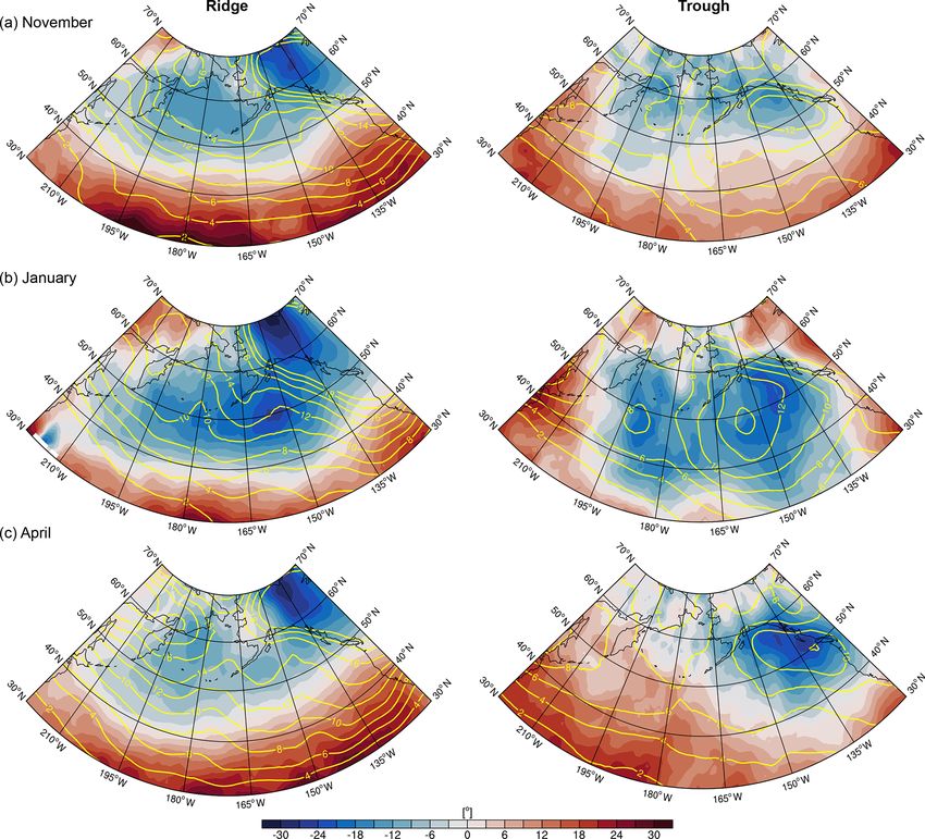
In Fig. 4a, a summary is given for the frequency of trough While all main upper-level storm tracks that are identi-
objects, the frequency of incipient trough age (yellow con- fied in earlier studies (Hoskins and Hodges, 2002) are also
tour in Fig. 4a) and the mean horizontal orientation (Fig. 4b)
Weather Clim. Dynam., 1, 459–479, 2020 https://doi.org/10.5194/wcd-1-459-2020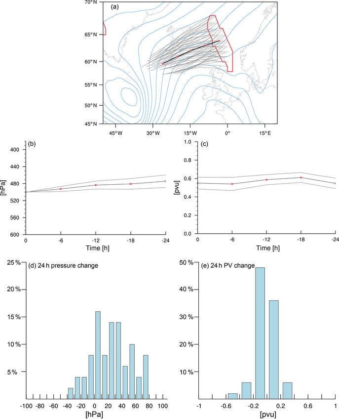
S. Schemm et al.: Life cycle of upper-level troughs and ridges                                                                            465

Figure 4. (a, c) Seasonal climatologies of the trough detection frequencies (color shading; units: %) for the cold (a; November–March) and
warm (c; May–September) seasons. Additional contours show selected frequencies of troughs with an age between 0 and 24 h (yellow).
(b, d) Seasonal climatologies of the corresponding horizontal trough orientation at the 500 hPa level (color shading; units: degrees) for the
cold (b; November–March) and warm (d; May–September) seasons. Positive values indicate anticyclonically oriented troughs. Additionally,
the yellow 0–24 h age contour, similar to that in (a, c), is shown for reference. The 1500 m height contour (black) is shown in all the panels.

successfully identified with our approach, there is surpris-              early troughs are recomputed based on the remaining trough
ingly no strong signal discernible along the southern branch              objects. These incipient troughs (yellow contour in Fig. 4a
over Eurasia highlighted by Chang and Yu (1999) and Chang                 indicates half of the maximum value in early trough de-
(2005). In principle, the algorithm is capable of picking up              tection frequency) are frequently detected downstream of
troughs and ridges near 25◦ N over Eurasia, as we confirmed               the Rocky Mountains and downstream of the Altai, sug-
by a manual inspection of cases, but the detection is less fre-           gesting that these two regions are preferred trough genesis
quent than one might expect. Potential reasons for this obser-            regions. There is also a smaller peak in the early trough
vation are discussed in the caveats section at the end of the             frequency near Greenland, suggesting that trough genesis
article.                                                                  also occurs near Greenland. However, the reduced trough
   The trough frequencies of incipient troughs are obtained               frequency compared to the Rocky Mountains suggests that
using the tracking capability of the algorithm (Sect. 2). To              Greenland troughs are indeed more transient. A second small
this end, all trough objects that are older than 1 d are re-              peak of early troughs is seen in the Gulf of Genoa, a pre-
moved from the data, and the detection frequencies of these               ferred region for Mediterranean cyclogenesis (Trigo et al.,

https://doi.org/10.5194/wcd-1-459-2020                                                       Weather Clim. Dynam., 1, 459–479, 2020
466                                                               S. Schemm et al.: Life cycle of upper-level troughs and ridges

2002). There are two additional, broader regions where early          of two compared to the trough detection frequency. For ex-
troughs are frequent and not linked to orography: the end of          ample, the ridge detection frequency downstream of Green-
the storm track over the North Pacific and over parts of north-       land with a preferred cyclonic orientation (Fig. 5b) is twice
ern Europe extending from the British Isles eastward across           as high as that for troughs. The band of enhanced ridge fre-
central Europe into Russia. It is plausible to think of these         quencies elongates downstream over the Nordic Seas, peaks
early troughs over Europe as a result of synoptic systems             over the Scandinavian Mountains and remains at a relatively
that decay upstream over the eastern North Atlantic. Wave             high level over Siberia. Upstream of the Altai, the ridge fre-
breaking and consecutive downstream developments at the               quency decreases, while downstream the trough frequency
end of a synoptic wave life cycle over the eastern North At-          peaks (Fig. 4a). Over large parts of Siberia, the ridges have
lantic then provide the seed for trough genesis further down-         no preferred orientation, while they tend to be anticycloni-
stream over Europe. Finally, a note of caution regarding the          cally oriented over East Asia. This band of higher ridge fre-
climatological trough age is in order. To obtain the age clima-       quencies might relate to the Siberian storm track – seen in
tology, the age information obtained from the trough track-           the track densities of 250 hPa meridional wind anomalies
ing is assigned to every grid point inside a two-dimensional          (Fig. 4a in Hoskins and Hodges, 2019) – while the main sur-
trough object, while points outside are labeled as missing            face storm track is located further poleward over the Barents
data. Time averaging of this field results in the mean age at         Sea region (Fig. 4a in Wernli and Schwierz, 2006). Over East
each grid point. The climatological age is therefore a func-          Asia and the western Pacific, the ridge detection frequency
tion of the trough size, and the age contours therefore enclose       is rather low, while the climatology over the Coast Moun-
smaller regions where troughs tend to be small. Furthermore,          tains of western North America is dominated by stationary
the number of troughs at each grid point varies according             ridges that preferentially have a cyclonic orientation (blue
to the trough frequency (color shading in Fig. 4a), and near          shading in Fig. 5b). Downstream of the Rocky Mountains,
the lateral boundaries of the domain a very low number of             ridge frequency is rather low. A smaller region of high early
troughs dictates the climatological mean. Late trough fre-            age ridge frequencies is found near Kamchatka (yellow con-
quencies typically encompass larger regions and extend fur-           tour in Fig. 5a), which indicates the presence of a transient
ther downstream (not shown), but the absolute frequency val-          ridge with a preferred cyclonic orientation (blue shading in
ues are considerably reduced.                                         Fig. 5b). Indeed, a local maximum in the surface cyclone fre-
   The trough orientation displays a strong zonal asymmetry.          quencies is found downstream of Kamchatka (see Fig. 4a in
Over the main oceanic storm tracks, the mean trough orienta-          Wernli and Schwierz, 2006). Overall, the trough and ridge
tion is preferentially cyclonic (blue shading in Fig. 4b). The        pattern alternates almost periodically in terms of the ampli-
cyclonic orientation increases toward the end of the storm            tude around the Northern Hemisphere.
tracks and also with latitude. Over land, the trough orien-              We further explored the role of the level and the min-
tation is preferentially anticyclonic. The anticyclonic orien-        imum lifetime of the detected features on the trough and
tation increases toward lower latitudes. This meridional de-          ridge frequencies. The trough and ridge detection patterns
pendence of the mean trough orientation is in agreement with          and the corresponding orientation at the 300 hPa level are in
the conventional interpretation of cyclonic and anticyclonic          very close agreement with the results at the 500 hPa level
wave life cycles and the associated wave breaking, which              (Fig. S1 in the Supplement). The detection frequencies are
occurs poleward (cyclonic) or equatorward (anticyclonic) of           increased everywhere by 10 %–20 %, but the main centers of
the mean jet position (Thorncroft et al., 1993). Over north-          action and the mean orientation agrees well between the lev-
ern Africa, the climatological trough orientation is strongly         els. We further computed the climatologies after removing
anticyclonic. In this region, troughs are frequently associ-          short-lived features that have a maximum lifetime of 24 h in
ated with anticyclonic wave breaking downstream of a ma-              a post-processing step (Supplementary Fig. S3). Again, the
ture extratropical cyclone situated off the Iberian Peninsula.        resulting patterns parallel those shown in Figs. 4 and 5, but
This downstream trough eventually thins and elongates equa-           the detection frequencies are reduced.
torward, corresponding to PV streamer formation. Eventu-
ally, an upper-level cutoff low forms. From the perspective           3.2   Extended summer (May–September)
of Rossby wave packets propagating along wave guides, the
anticyclonic troughs in this sector have been described as the        The pattern in the trough detection frequencies changes from
transmitters between wave packets initiated on the subtrop-           winter to summer (Fig. 4). Over North America, the main
ical wave guide (i.e., the jet over northern Africa) by wave          frequency peak is located downstream of the Great Lakes
packets that propagate along the extratropical wave guide             Region and over Newfoundland, while it was previously lo-
over the North Atlantic (Martius et al., 2010, in particular,         cated further upstream. This is in agreement with the high
their Fig. 5).                                                        surface cyclone frequencies seen in summer in this region
   In Fig. 5a, a summary is given for the number of ridges de-        (see Fig. 4c in Wernli and Schwierz, 2006). Over the North
tected during the cold season. Remarkably, the ridge detec-           Atlantic, the main frequency peak is located just off the
tion frequency over many regions is larger by almost a factor         Iberian Peninsula. There is no comparable peak in surface

Weather Clim. Dynam., 1, 459–479, 2020                                                   https://doi.org/10.5194/wcd-1-459-2020
S. Schemm et al.: Life cycle of upper-level troughs and ridges                                                                      467

Figure 5. Similar to Fig. 4 but for ridges. The dashed contour indicates the region where the ridge frequency is above the maximum global
trough detection frequency (≈ 16 %).

cyclone frequencies in this region, so the flow conditions             situation is also shown in Fig. 5.7 of Martius and Rivière
will result in the formation of a cut-off low with no well-            (2016).
marked surface signature. Surface cyclone frequencies have                Over Eurasia, a maximum in the summertime detection
a peak downstream of Greenland (see Fig. 4c in Wernli and              frequencies of troughs connects the Eastern Mediterranean
Schwierz, 2006), but there is no maximum trough frequency              with the Black Sea. This feature is not well reproduced in
there. However, upper-level storm-track measures – based               Rossby wave-breaking climatologies of which we are aware,
on, for example, track densities of 250 hPa vorticity – in-            but it is clearly seen in the upper-level track densities in vor-
deed indicate the presence of a trough-like feature off the            ticity on 250 hPa (Hoskins and Hodges, 2019). Furthermore,
Iberian Peninsula during summer (see Fig. 1c in Hoskins                this local maximum corresponds to a similar maximum seen
and Hodges, 2019). Because a similar feature is also seen              in summertime climatologies of stratospheric PV streamers
in summertime climatologies of Rossby wave breaking (see               (see Fig. 6b in Wernli and Sprenger, 2007). PV streamers
Fig. 10a in Postel and Hitchman, 1999), we expect this maxi-           form a subcategory of troughs and are best described as
mum in trough frequency to be related to anticyclonic Rossby           filament-like elongated troughs, which have a length that is
wave breaking, as described for the LC1 scenario in Fig. 12a           longer than their width (Wernli and Sprenger, 2007). Stream-
of Thorncroft et al. (1993). An example of such a synoptic             ers are associated with anticyclonic Rossby wave breaking,
                                                                       so it is not too surprising that the detection hot spots off the

https://doi.org/10.5194/wcd-1-459-2020                                                   Weather Clim. Dynam., 1, 459–479, 2020
468 S. Schemm et al.: Life cycle of upper-level troughs and ridges
Iberian Peninsula and near the Black Sea eventually become high-pass filtered wind data,
part of the same Rossby wave train (see, for example, Fig. 3
in Wernli and Sprenger, 2007, for such a synoptic situation). " #
1
v ∗2 − u∗2
A second maximum over Eurasia is located west of 90◦ E, a E= 2 , (2)
feature seen again in the streamer climatology of Wernli and −u∗ v ∗
Sprenger (2007). Further east, the maximum over East Asia
exhibits only weak changes in its location between winter where the overbar indicates a time average and the asterisks
(Fig. 4a) and summer (Fig. 4c) but appears with a reduced a deviation from the time average. The fundamental relation-
amplitude during summer. Finally, over the northeastern Pa- ships between the trough and ridge orientation and the eddy
cific, the summer maximum is shifted slightly equatorward momentum flux were discussed in the early 20th century by
compared to its position during winter. It is located off the Jeffreys (1926) and Starr (1948). As summarized in the Intro-
US west coast during summer, while it is located in the Bay duction, equatorward-pointing E vectors are assumed to in-
of Alaska during winter. This is a counterintuitive result be- dicate anticyclonically oriented eddies (Rivière et al., 2003)
cause storm tracks generally tend to shift poleward during associated with a more poleward eddy momentum flux. Dur-
summer (Hoskins and Hodges, 2019). ing El Niño, the situation is essentially the opposite: eddies
The ridge frequency pattern over North America contin- downstream of the Rocky Mountains exhibit a more cyclonic
ues to be dominated by the stationary ridges over the Coast orientation and tend to push the North Atlantic jet equa-
Mountains despite a mild reduction in the absolute detection torward, as is suggested by more poleward-oriented E vec-
frequencies (color shading in Fig. 5c). tors. The Pacific and North Atlantic jets are more zonally
Finally, we note that – as is the case for the winter season – extended, which tends to increase extratropical cyclogenesis
the results obtained at the 300 hPa level (Fig. S1) are in very over the Gulf Stream (Schemm et al., 2016). To shed further
close agreement with those at the 500 hPa level. The 300 hPa light on this, we therefore explore the ENSO climatologies
detection frequencies are moderately higher, but the patterns using troughs and ridges, which are very closely related to
are remarkably similar. the upper-level eddies described above.
In Fig. 6, anomalies in the orientation of troughs and ridges
are shown for ENSO-affected winter seasons based on the
Oceanic Niño Index (ONI) from NOAA’s Climate Predic-
3.3 ENSO-affected winter seasons tion Center. During El Niño (Fig. 6a), troughs and ridges ex-
hibit a stronger cyclonic orientation over the northeastern Pa-
cific, North America and the North Atlantic. The anomalies
The influence of the ENSO on the midlatitudes is a long- are strongest over the northeastern Pacific and off the east
standing research topic – for recent reviews, we refer the coast of the US. Over the North Atlantic, the stronger-than-
reader to publications by Liu and Alexander (2007), Stan usual cyclonic orientation is most pronounced along 30◦ N,
et al. (2017), and Yeh et al. (2018). Recently, particu- which is about the latitude of the zonally more extended jet
lar progress has been made in understanding the role of in this region during El Niño. In contrast, during La Niña,
synoptic-scale eddies in shaping the North Atlantic circula- troughs and ridges exhibit a more anticyclonic orientation
tion response to ENSO. More specifically, there is increasing over the northeastern Pacific, North America and parts of
evidence that the North Atlantic teleconnection pattern is in the North Atlantic. These results are in agreement with those
part a downstream response of the eddy-driven jet to changes from the previous studies that rely on the strength and orien-
in the orientation of synoptic-scale eddies entering the North tation of the E vectors. The results are also in good agree-
Atlantic from North America (Li and Lau, 2012a, b; Drouard ment with the findings of Shapiro et al. (2001), who noted
et al., 2015). The mechanisms can be briefly summarized more life cycles of type LC2 (cyclonic) over the Pacific dur-
as follows (for a schematic summary, see also Fig. 13 in ing El Niño and more life cycles of type LC1 (anticyclonic)
Schemm et al., 2018): in response to an amplified ridge over during La Niña. The trough and ridge detection and track-
the northeastern Pacific during La Niña, upper-level synoptic ing algorithm can thus enrich insights into the dynamics of
eddies with a more anticyclonic orientation form downstream upper-level eddies during ENSO-affected winters. For ex-
of the Rocky Mountains, where lee cyclogenesis is also en- ample, the anomalies during El Niño over the northeastern
hanced. These eddies propagate downstream over the North Pacific are predominantly due to more cyclonically oriented
Atlantic while maintaining their anticyclonic orientation un- troughs, while the anomalies over the North Atlantic have a
til anticyclonic wave breaking occurs over the eastern North stronger signal in the ridge anomalies (not shown). The more
Atlantic. Anticyclonic wave breaking pushes the eddy-driven cyclonic trough and ridge orientation over the Pacific is con-
jet poleward. Until now, the anomalous anticyclonic orienta- nected to the deepening of the Aleutian Low during El Niño,
tion and the associated more poleward eddy momentum flux whereas it is a strong Aleutian High during La Niña that is
were diagnosed using the horizontal E vectors of Hoskins in agreement with more anticyclonic troughs and ridges (Mo
et al. (1983) and Trenberth (1986), which are obtained using and Livezey, 1986).
Weather Clim. Dynam., 1, 459–479, 2020 https://doi.org/10.5194/wcd-1-459-2020S. Schemm et al.: Life cycle of upper-level troughs and ridges 469
Figure 6. Averaged orientation anomalies (units: degrees) of 500 hPa troughs and ridges during (a) El Niño- and (b) La Niña-affected winter
seasons. Negative (positive) anomalies indicate more cyclonically (anticyclonically) oriented troughs and ridges compared to the seasonal
climatology. Regions where the detection frequency is below 2 % are excluded.
3.4 The North Pacific storm track in midwinter 2013; Afargan and Kaspi, 2017). This is also the case in ide-
alized aqua planet simulations (Novak et al., 2020).
The equatorward shift of the subtropical jet over the Pa-
The midwinter suppression of the North Pacific storm track
cific changes the large-scale environment in which synoptic
intensity is another research topic that has recently received
systems grow because more systems will grow on the pole-
renewed attention. While the mean baroclinicity is largest
ward flank of the jet. The poleward flank is characterized by
during midwinter, storm track activity is reduced over the
a large-scale cyclonically sheared environment. According to
North Pacific – in contrast to the North Atlantic (Nakamura,
idealized wave life cycles (Thorncroft et al., 1993), we must
1992). As feature-based tracking statistics have shown, the
expect more cyclonic (LC2) developments during midwin-
suppression is connected to a reduced eddy intensity and
ter. Indeed, troughs and ridges at the 500 hPa level exhibit a
upper-level eddy frequency (Penny et al., 2010), while it
stronger cyclonic orientation in January (Fig. 7b) compared
does not affect the frequency of surface eddies (Schemm
to, for example, November and April (Fig. 7a and c). Not
and Schneider, 2018). Several mechanisms have been sug-
only does the mean cyclonic orientation increase during mid-
gested to contribute to the suppression, for example, a re-
winter but also wider parts of the Pacific are affected by cy-
duction in upstream seeding (Penny et al., 2010, 2011, 2013;
clonically oriented troughs and ridges. In particular, in Jan-
Chang and Guo, 2011, 2012) or an increase in the jet speed
uary, cyclonic troughs dominate the North Pacific even equa-
with a concomitant reduction in the jet width (Harnik and
torward of 40◦ N, which is not the case in November and
Chang, 2004). Recently, however, several studies have high-
April.
lighted the important role of processes internal to the North
There are several observations based on trough and ridge
Pacific storm track, such as a reduction in the lifetime of
detection that may prove useful in gaining a better under-
eddies (Schemm and Schneider, 2018) and an increase in
standing of the midwinter suppression. First, there is no
the eddy group velocity (Chang, 2001). There is growing
marked reduction in the frequency of troughs and ridges dur-
evidence that the equatorward shift in the subtropical jet is
ing midwinter, as is the case for high-pass-filtered eddies at
key for understanding the suppression (Chang, 2001; Naka-
the same height (Penny et al., 2010)1 . A local increase in
mura and Sampe, 2002; Yuval et al., 2018; Schemm and Riv-
trough frequency over the eastern Pacific is observed (yel-
ière, 2019). When the subtropical jet over the Pacific shifts
low contours in Fig. 7c, right column) and an overall pole-
equatorward, the efficiency of synoptic systems to convert
ward movement of the ridge frequencies, which otherwise do
the mean baroclinicity into eddy energy is reduced due to a
not display a well-marked reduction. Second, the preferred
change in the vertical eddy structure (Chang, 2001; Schemm
trough and ridge orientation is cyclonic during midwinter,
and Rivière, 2019). The tilt of the eddy geopotential isolines
with two maxima over the eastern and western Pacific (right
with height – which is more poleward when the eddy effi-
column in Fig. 7b), which indicates a consistent change in
ciency decreases during midwinter – is constrained by the
the character of synoptic wave life cycles during midwinter.
eddy propagation direction, which is more shifted toward the
The first maximum between 40–50◦ N, 165–180◦ E is colo-
Equator during midwinter (Schemm and Rivière, 2019; No-
vak et al., 2020); see, for example, Figs. 1 and 8 in Schemm
and Rivière (2019). Equatorward jet shifts also reduce the 1 Note that Penny et al. (2010) use a 90 d high-pass filter plus a
storm track intensity over the North Atlantic (Penny et al., spatial filter that admits only wavenumbers 5 to 42.
https://doi.org/10.5194/wcd-1-459-2020 Weather Clim. Dynam., 1, 459–479, 2020470 S. Schemm et al.: Life cycle of upper-level troughs and ridges Figure 7. Monthly mean orientation (color shading; degrees) and frequency (yellow contours, from 2 % to 14 % in steps of 2 %) of 500 hPa ridges and troughs during (a) November, (b) January and (c) April over the North Pacific. cated with the region of maximum reduction in the efficiency because – as was shown in a previous section – maxima in the of baroclinic growth (see Fig. 2b in Schemm and Rivière, trough frequency exhibit a strong agreement with maxima in 2019) and slightly upstream of the maximum in eddy ki- cyclosis (compared with, for example, Fig. 5d in Hoskins and netic energy (see Fig. 1 in Schemm and Schneider, 2018), Hodges, 2002). Thus, the conversion rates and eddy kinetic which is suppressed during midwinter. Because the cyclonic energy (EKE) are reduced downstream of the maximum cy- orientation of troughs and ridges is typically strongest dur- clonic orientation of the upper-level troughs compared to the ing the final stage of a synoptic wave life cycle, a plausible shoulder seasons. Indeed, a reduction in the lifetime of syn- – but here untested – hypothesis for the existence of the first optic systems is observed during midwinter (Schemm and maximum would be that synoptic cyclones generated east of Schneider, 2018). The second maximum is related to the de- Japan over the Kuroshio extension have an accelerated life cay of the synoptic waves at the exit of the Pacific storm track cycle with a fast and intense deepening phase followed by in the Bay of Alaska. a rapid decay, resulting in a reduced life time as found by Schemm and Schneider (2018). The enhanced lysis over the eastern Pacific is in agreement with the localized trough fre- quency maximum (yellow contours in Fig. 7c, right column), Weather Clim. Dynam., 1, 459–479, 2020 https://doi.org/10.5194/wcd-1-459-2020
S. Schemm et al.: Life cycle of upper-level troughs and ridges                                                                 471

4   Lagrangian perspective on troughs and ridges                   reflects the nature of the air mass motion inside troughs in
                                                                   which equatorward-moving air mildly descends due to the
In this section, we show how trough and ridge detection can        quasi-isentropic down-glide, while in some cases vigorous
be used to investigate trough and ridge dynamics from a            vertical motions occur – in agreement with the long tail to-
Lagrangian perspective. To this end, we couple the trough          ward positive values of the potential temperature distribution
and ridge detection with a Lagrangian analysis using LA-           (Fig. 9e and f). We refer to the descending motion as quasi-
GRANTO (Wernli and Davies, 1997; Sprenger and Wernli,              isentropic because for most trajectories a mild decrease in
2015), which we use to compute air parcel trajectories from        potential temperature between −2 and 0 K is found, likely
detected trough and ridge features.                                resulting from radiative cooling. Most of these air parcels are
   The procedure is best explained with a simple example           associated with only small changes in pressure. The overall
(Fig. 8). At 18:00 UTC on 18 January 2010, a trough is de-         asymmetry in the pressure change distribution ultimately re-
tected over the Nordic Seas downstream of a mature low-            lates to the occurrence of upward moist convection and the
pressure system south of Greenland (Fig. 8a). The trough has       impact of condensation on the vertical motion in the atmo-
a mildly cyclonic orientation and will broaden during the fol-     sphere. This skewness is thus a general feature of extratrop-
lowing days. A potential research question may be whether          ical cyclones in a moist atmosphere (O’Gorman, 2011). The
the formation of this downstream trough is predominately           skewness and asymmetry is assumed to increase in a warmer
driven by dry dynamics or considerably modified by diabatic        climate and with increasing moisture content (Booth et al.,
processes. To answer this, air parcel trajectories are released    2015; Tamarin-Brodsky and Hadas, 2019; Sinclair et al.,
from every grid point inside the trough feature (thin gray         2020). The trajectories associated with strong vertical mo-
lines in Fig. 8a), which highlight the pathway of air parcels      tion all originate in the boundary layer and first increase and
that constitute the trough at the 500 hPa level. The mean evo-     later decrease their potential vorticity (not shown), which is
lutions of pressure (Fig. 8b) and PV (Fig. 8c) along these         characteristic of a warm conveyor belt ascending ahead of
parcel trajectories suggest that the air is mostly advected hor-   the trough axis (e.g., Wernli and Davies, 1997). These cases
izontally with a minor descent of approximately 20 hPa in          exhibit a marked increase in potential temperature, which
24 h. Further, the diabatic modification of PV during the 24 h     reflects the cross-isentropic motion. For the few cases with
prior to arrival in the target region is small. The mean po-       a strong decrease larger than 200 Pa in 24 h, we find that
tential temperature (not shown) decreases during this period       the vast majority of the parcels – originating between 200–
from 297 to 295 K. While the mean values suggest only little       300 hPa – decrease their potential vorticity. Only a small
change in pressure and PV, the histograms of 24 h changes in       fraction of approximately 1 % starts with stratospheric val-
pressure and PV show that around 15 % of the air descends          ues (> 2 pvu), but we assume that this number increases
during the 24 h period by up to 60–80 hPa (Fig. 8d) and that       for 300 hPa troughs. Finally, we note that the 24 h pressure
a small fraction of less than 5 % decrease their PV by more        change for July is even more confined to values between
than 0.4 pvu2 (Fig. 8e). Thus, the dynamics underlying the         0–100 hPa, while the 24 h change in potential vorticity is
formation of this specific downstream trough at this stage of      more confined between −0.2 and 0.2 pvu, which is a result
its life cycle are mostly dry and therefore can be approxi-        that reflects the overall more intense cyclone and associated
mated by the traditional paradigm of downstream develop-           trough–ridge development and vertical motion during winter.
ment (Simmons and Hoskins, 1979; Simmons, 1999; Orlan-                For the 500 hPa ridges, the histogram of changes in pres-
ski and Chang, 1993; Papritz and Schemm, 2013). However,           sure along the flow of 24 h backward parcel trajectories is
for a small embedded fraction of air, much stronger descent        centered between −100 and 0 hPa, again with a longer tail
and diabatic PV modification than indicated by the mean are        toward negative values (Fig. 10). It is therefore shifted more
observed.                                                          toward negative values than the trough histogram, which re-
   Next, 24 h backward trajectories are released from all de-      flects the quasi-isentropic up-glide of air moving poleward
tected troughs and ridges over the North Atlantic (60–0◦ W,        and upward in a ridge. The pressure change in July is again
20–70◦ N) in 1 winter and 1 summer month: January 2010,            more shifted toward negative values (ascent) than the trough
when more than 25 000 parcel trajectories are released, and        histogram but is centered around −50 and 50 hPa. If our in-
July 2010, with more than 16 000 parcel trajectories. The          terpretation is correct, the histograms are dominated by the
binned 24 h changes for pressure, potential vorticity and          almost isentropic motion of air inside troughs and ridges, and
potential temperature are presented in Fig. 9. During Jan-         the reduced pressure change along the flow in July relative to
uary 2010, the distribution of 24 h pressure changes is cen-       January reflects the reduced baroclinicity or isentropic tilt in
tered between 0–100 hPa (corresponding to a weak descent)          summer compared to winter, in combination with a reduced
and is highly skewed toward negative values (corresponding         wind speed according to the thermal wind relationship. It is,
to a strong ascent) of up to −500 hPa, in contrast to pos-         however, important to note that the histograms of potential
itive values that do not exceed 250 hPa. This phenomenon           temperature and vorticity changes show that the motion is
                                                                   not fully dry adiabatic. The histograms of potential vorticity
    2 1 pvu = 10−6 m2 s−1 K kg−1 .                                 changes are symmetrically distributed around zero with out-

https://doi.org/10.5194/wcd-1-459-2020                                               Weather Clim. Dynam., 1, 459–479, 2020
You can also read