RECOG RL01: correcting GRACE total water storage estimates for global lakes/reservoirs and earthquakes - mediaTUM
←
→
Page content transcription
If your browser does not render page correctly, please read the page content below
Earth Syst. Sci. Data, 13, 2227–2244, 2021
https://doi.org/10.5194/essd-13-2227-2021
© Author(s) 2021. This work is distributed under
the Creative Commons Attribution 4.0 License.

           RECOG RL01: correcting GRACE total water storage
          estimates for global lakes/reservoirs and earthquakes
             Simon Deggim1 , Annette Eicker1 , Lennart Schawohl1 , Helena Gerdener2 , Kerstin Schulze2 ,
               Olga Engels2 , Jürgen Kusche2 , Anita T. Saraswati3 , Tonie van Dam4 , Laura Ellenbeck5 ,
          Denise Dettmering5 , Christian Schwatke5 , Stefan Mayr6 , Igor Klein6 , and Laurent Longuevergne7
                 1 Geodesy    & Geoinformatics, HafenCity University Hamburg, 20457 Hamburg, Germany
                   2 Institute of Geodesy and Geoinformatics, University of Bonn, 53012 Bonn, Germany
                   3 Department of Engineering, University of Luxembourg, 4364 Luxembourg, Luxembourg
         4 Interdisciplinary Centre for Security, Reliability and Trust, University of Luxembourg, 1359 Luxembourg,

                                                           Luxembourg
        5 Deutsches Geodätisches Forschungsinstitut, Technical University of Munich (DGFI-TUM), 80333 Munich,

                                                             Germany
               6 Earth Observation Center, German Aerospace Center (DLR), 82234 Oberpfaffenhofen, Germany
                    7 CNRS, Geosciences Rennes – UMR 6118, Université de Rennes, 35000 Rennes, France

                 Correspondence: Simon Deggim (simon.deggim@hcu-hamburg.de) and Annette Eicker
                                              (annette.eicker@hcu-hamburg.de)

                                 Received: 28 August 2020 – Discussion started: 22 October 2020
                            Revised: 12 April 2021 – Accepted: 14 April 2021 – Published: 21 May 2021

      Abstract. Observations of changes in terrestrial water storage (TWS) obtained from the satellite mission
      GRACE (Gravity Recovery and Climate Experiment) have frequently been used for water cycle studies and
      for the improvement of hydrological models by means of calibration and data assimilation. However, due to a
      low spatial resolution of the gravity field models, spatially localized water storage changes, such as those occur-
      ring in lakes and reservoirs, cannot properly be represented in the GRACE estimates. As surface storage changes
      can represent a large part of total water storage, this leads to leakage effects and results in surface water signals
      becoming erroneously assimilated into other water storage compartments of neighbouring model grid cells. As
      a consequence, a simple mass balance at grid/regional scale is not sufficient to deconvolve the impact of sur-
      face water on TWS. Furthermore, non-hydrology-related phenomena contained in the GRACE time series, such
      as the mass redistribution caused by major earthquakes, hamper the use of GRACE for hydrological studies in
      affected regions.
         In this paper, we present the first release (RL01) of the global correction product RECOG (REgional COrrec-
      tions for GRACE), which accounts for both the surface water (lakes and reservoirs, RECOG-LR) and earthquake
      effects (RECOG-EQ). RECOG-LR is computed from forward-modelling surface water volume estimates derived
      from satellite altimetry and (optical) remote sensing and allows both a removal of these signals from GRACE and
      a relocation of the mass change to its origin within the outline of the lakes/reservoirs. The earthquake correction,
      RECOG-EQ, includes both the co-seismic and post-seismic signals of two major earthquakes with magnitudes
      above Mw 9.
         We discuss that applying the correction dataset (1) reduces the GRACE signal variability by up to 75 %
      around major lakes and explains a large part of GRACE seasonal variations and trends, (2) avoids the in-
      troduction of spurious trends caused by leakage signals of nearby lakes when calibrating/assimilating hy-
      drological models with GRACE, and (3) enables a clearer detection of hydrological droughts in areas af-
      fected by earthquakes. A first validation of the corrected GRACE time series using GPS-derived vertical
      station displacements shows a consistent improvement of the fit between GRACE and GNSS after apply-

Published by Copernicus Publications.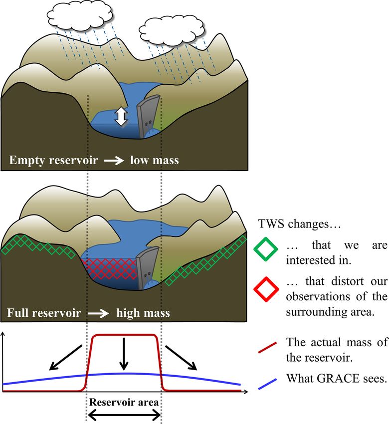
2228                                                              S. Deggim et al.: GRACE correction product RECOG RL01

       ing the correction. Data are made available on an open-access basis via the Pangaea database (RECOG-
       LR: Deggim et al., 2020a, https://doi.org/10.1594/PANGAEA.921851; RECOG-EQ: Gerdener et al., 2020b,
       https://doi.org/10.1594/PANGAEA.921923).

1   Introduction

The dynamic global water cycle influences our everyday
lives by affecting freshwater availability, weather/climate
fluctuations and trends, seasonal variations, anthropogenic
water use, and single extreme events such as floods and
droughts. Understanding how water is transiently stored and
exchanged among the different compartments (groundwater,
surface water, soil moisture, etc.) with the help of hydrologi-
cal models is, therefore, of major societal importance. How-
ever, large model uncertainties caused by errors in climate
forcings and an incomplete realism of process representa-
tions limit the models’ ability to accurately simulate water
storages and fluxes, making independent observations indis-
pensable for model validation/calibration and data assimila-
tion.
   Since 2002 measurements of time-variable gravity ob-
tained from the twin-satellite mission GRACE (Gravity Re-
covery and Climate Experiment; Tapley et al., 2004) and its
successor mission GRACE-Follow-On (GRACE-FO; Flecht-
ner et al., 2016; Kornfeld et al., 2019) have allowed for the
determination of column-integrated terrestrial water storage
(TWS) changes on a global scale with uniform data coverage         Figure 1. Overview of the lake leakage problem with localized
(e.g. Pail et al., 2015). However, several challenges are in-      changes in water level of the lake/reservoir influencing the esti-
volved with using GRACE for improving hydrological mod-            mated water storage in surrounding areas.
els, among them (1) the low spatial resolution of GRACE,
integrating spatially over regions as large as ∼ 200 000 km2
and hampering the representation of concentrated and sub-          at the location of their origin and with the correct magnitude.
scale water storage changes, and (2) the fact that gravity         Thus they can distort the water storage estimate for neigh-
observations also contain non-hydrology-related mass vari-         bouring areas or the average over a river basin, as shown in
ations.                                                            Fig. 1.
   The first problem is caused by the GRACE orbit configu-            This sub-scale mass variability impacts GRACE am-
ration in combination with unmodelled short-periodic mass          plitudes up to 20 % averaged over basins as large as
changes, resulting in the gravity field models being strongly      ∼ 200 000 km2 (Longuevergne et al., 2013; Farinotti et al.,
corrupted by spatially correlated noise. The necessary spa-        2015). Although the issue of concentrated hydrological mass
tial filtering approach (e.g. Kusche, 2007) inevitably leads to    variations is not limited to surface waterbodies (e.g. Castel-
signal loss and to leakage effects resulting in a rather coarse    lazzi et al., 2018), dam operations and impoundment have a
spatial resolution of the gravity field models of a few hundred    large impact on the water cycle and on continent–ocean ex-
kilometres.                                                        changes (Chao et al., 2008). Therefore, several publications
   This limits the investigation of mass variations to rather      have focused on removing the impact of surface waterbod-
large-scale processes (Longuevergne et al., 2013), even            ies from GRACE total water storage changes. For example,
though small-scale mass variations, whose typical size is          Grippa et al. (2011) removed the influence of surface wa-
smaller than GRACE resolution but large enough in mag-             ter storage in the Niger River (derived from altimetry and
nitude, can have a strong influence on the total mass              remotely sensed surface water extent) from GRACE TWS
change signal (Frappart et al., 2012). Examples are human-         estimates to better be able to compare them to hydrological
controlled reservoirs or natural lakes with strong (seasonal)      model output. Tseng et al. (2016) determined mass changes
variations and/or trends. Even though GRACE can “see”              in two Tibetan lakes, combining altimetry, remote sensing,
these mass changes, they do not necessarily appear exactly         and GRACE estimates, and Zhang et al. (2017) estimated

Earth Syst. Sci. Data, 13, 2227–2244, 2021                                          https://doi.org/10.5194/essd-13-2227-2021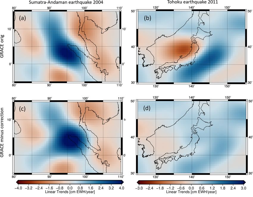
S. Deggim et al.: GRACE correction product RECOG RL01                                                                        2229

water volume changes for 96 % of the lake area on the Ti-          sensing data (e.g. Schwatke et al., 2020; Busker et al., 2019;
betan Plateau by combining an average of ICESat-derived el-        Crétaux et al., 2011).
evation changes from a number of larger lakes with Landsat            To account for the second challenge in using GRACE
lake area changes for smaller lakes. Ni et al. (2017) removed      data for hydrological studies, namely the removal of all non-
the leakage error in GRACE estimates over Lake Volta in            hydrology-related mass variations, some effects are typically
Ghana using constrained forward modelling. All these stud-         subtracted using geophysical models either during the com-
ies represent regional test cases, but a global assessment of      putation of the gravity field solutions (e.g. Earth tides, ocean
the influence of surface waterbody mass change on GRACE            tides, and oceanic/atmospheric mass variations) or in post-
data is missing.                                                   processing (e.g. glacial isostatic adjustment (GIA)). How-
   Using GRACE data for the evaluation of (global) hydro-          ever, in addition to this, the mass redistribution caused by
logical models or for combining models and observations by         the crustal deformation following large earthquakes is also
model calibration (Werth and Güntner 2010) and data assimi-        contained in the GRACE observations masking hydrologi-
lation (C/DA; Zaitchik et al., 2008; Eicker et al., 2014) with-    cal phenomena in the affected regions. Several studies have
out accounting for localized surface water storage can lead        highlighted GRACE’s usefulness for estimating large earth-
to two different kinds of errors. (i) Many global hydrologi-       quakes (Mw > 9.0; e.g. Panet et al., 2007; Broerse, 2014;
cal models do not include a surface water storage compart-         Einarsson et al., 2010; Einarsson, 2011; L. Wang et al., 2012)
ment at all (Scanlon et al., 2017), and assimilating GRACE         and have also identified co- and post-seismic earthquake sig-
TWS into a model that does not explicitly include surface          nals in GRACE data with a lower magnitude (e.g. Han et
waters will inevitably result in other storage compartments        al., 2016; Zhang et al., 2016), down to magnitude 8.3 (Chao
(such as soil moisture or groundwater) becoming distorted          and Liau, 2019). For example, the onset of the Sumatra–
by absorbing the observed surface water mass change. Even          Andaman earthquake in December 2004 (magnitude 9.1) was
if a model such as WaterGAP (Müller Schmied et al., 2014)          analysed using, among others, differences of monthly grav-
does include a surface water compartment, it might not repre-      ity solutions (Han et al., 2006), wavelet analysis (Panet et
sent the realistic behaviour of, for example, human-operated       al., 2007), Bayesian approaches (Einarsson et al., 2010), or
reservoirs, and it might be preferable to exclude the reservoir    normal modes (Cambiotti et al., 2011). At time of writing,
storage from the assimilation. (ii) The leakage effect of lo-      the German GeoForschungsZentrum in Potsdam (GFZ) is
calized surface waterbodies might cause an assimilation of         the only processing centre that provides a total water stor-
the surface water mass change into neighbouring grid cells         age (level 3) dataset corrected for earthquakes (Boergens et
that should not be affected by it. To our knowledge, no inves-     al., 2019); however, a data-based global earthquake correc-
tigation so far has studied the effects of surface waterbodies     tion for different GRACE solutions is not available yet.
on GRACE model calibration or data assimilation and how               To account for both the localized surface water storage
they can best be handled in order to not distort the C/DA          in lakes/reservoirs and the earthquake signal, we present the
results. Having a global correction dataset to clear GRACE         first release of a new global correction dataset, RECOG (RE-
water mass changes of the influence of large surface water-        gional COrrections for GRACE) RL01, which can be used
bodies (here, lakes and reservoirs) will be immensely helpful      for disaggregation of the integral GRACE water storage es-
for making GRACE estimates more consistent with model              timates in addition to applying standard corrections such as
output.                                                            GIA models and the atmosphere/ocean de-aliasing products.
   Today, extensive information on surface water variations is     The term RECOG refers to the fact that all effects included
available from satellite remote sensing. For almost 30 years,      in the data product are localized phenomena that neverthe-
satellite altimetry has been providing water levels of large       less influence a larger region around them. The surface wa-
and medium lakes and reservoirs on a global scale (e.g. Bir-       ter correction (RECOG-LR) was computed from forward-
kett, 1995; Berry et al., 2005; Göttl el al., 2016). Several       modelling altimetry and remote sensing observations and can
databases make these time series freely available for hydro-       be used (a) to subtract the lake/reservoir storage from the
logical applications, among them the Database for Hydrolog-        GRACE time series (removal approach) and (b) to relocate
ical Time Series of Inland Waters (DAHITI; Schwatke et al.,        the surface water storage at its exact location of origin (relo-
2015). In addition, optical satellite images are used to derive    cation approach). The earthquake correction (RECOG-EQ)
surface extent of lakes and reservoirs (e.g. Pekel et al., 2016;   was estimated from GRACE monthly solutions using the
Klein et al.,2017; Schwatke et al., 2019). Time series from        Bayesian approach provided in Einarsson et al. (2010) and
optical sensors can reach a length of up to almost 40 years        takes into account both the co-seismic and the post-seismic
with a spatial resolution of 250 (MODIS, since 1999), 30           signal.
(Landsat, since 1982), and 10 m (Sentinel-2, since 2015) as           This paper is organized as follows: Sect. 2 describes the
well as a high temporal resolution with revisit time from 14       input data and processing steps, presents the resulting cor-
(Landsat), over 5 (Sentinel-2), and up to 1 d (MODIS). By          rection products, and visualizes some of its key character-
combining height and surface area information, time series         istics. In Sect. 3 we then show different exemplary applica-
of storage changes can be derived purely based on remote           tions of the dataset in order to illustrate its impact and to

https://doi.org/10.5194/essd-13-2227-2021                                         Earth Syst. Sci. Data, 13, 2227–2244, 2021
2230                                                              S. Deggim et al.: GRACE correction product RECOG RL01

demonstrate its value: influence of RECOG on GRACE time            an extended outlier detection before and after data combina-
series including a short discussion of the impact on data as-      tion, including an optional classification of the radar echoes.
similation into a global hydrological model, the detection of      The temporal resolution of the time series differs depending
drought indices in an earthquake-affected region, and a val-       on the size of a lake. Small lakes that are only covered by
idation of the correction product using GNSS-observed sta-         one single satellite track can be measured every 35 or 10 d
tion displacements. This is followed by a discussion of the        (depending on the mission), whereas for large lakes a height
benefits and limitations of the correction product in Sect. 4,     can be derived almost every day. Moreover, information can
before Sect. 5 summarizes the findings and gives an outlook        only be provided for those waterbodies located directly be-
on further development options.                                    neath a satellite’s tracks (Dettmering et al., 2020), prevent-
                                                                   ing the creation of water level time series of small lakes lo-
                                                                   cated between the satellites’ ground tracks. In addition, for
2     Methods and results                                          small lakes or lakes surrounded by large topography no reli-
                                                                   able height information might be created due to corrupted or
In this section we describe the various input data and their       too-noisy radar echoes.
sources (Sect. 2.1.1 and 2.1.2) that were used to perform the         The quality of the DAHITI water level time series depends
forward modelling (Sect. 2.1.4) of the surface waterbodies         on various criteria, mainly on the size of the lake and the
and its necessary pre-processing steps (Sect. 2.1.3). The re-      length of the crossing satellite track as well as the surround-
sulting lake/reservoir correction dataset, RECOG-LR, is dis-       ing topography. Comparison with in situ data show RMSE
cussed in Sect. 2.1.5. The processing steps for computing the      of a few centimetres for larger lakes and RMSE of some
earthquake correction are described in Sect. 2.2.1, followed       decimetres for river crossings (Schwatke et al., 2015).
by the results of RECOG-EQ (Sect. 2.2.2).

                                                                   2.1.2   Creating lake shapes from remote sensing
2.1     Lake/reservoir correction, RECOG-LR
                                                                   Based on MODIS optical satellite data, daily surface water
The lake/reservoir correction is based on a subset of currently    extents are provided by the DLR’s Global WaterPack (GWP)
283 of the largest surface waterbodies monitored with satel-       product (Klein et al., 2017). To receive reliable estimates of
lite altimetry (see Supplement S1 for a complete list). The        the extent of large global lakes and reservoirs, daily obser-
lake water volume variations product is designed around (1)        vations are aggregated to obtain maximum waterbody ex-
monthly water level time series from a global multi-satellite      tents for the years 2003 to 2018. To capture coherent water-
product and (2) the (static) surface water extent area for each    bodies, a pixel-based region-growing algorithm is applied,
lake.                                                              using ancillary information of the temporal static Hydro-
                                                                   LAKES dataset (Messager et al., 2016) for waterbody iden-
2.1.1    Lake level time series from altimetry                     tification. Hereby, every water pixel in the aggregated GWP
                                                                   raster layer that spatially overlaps with the original Hydro-
Satellite altimetry measures the distance between the satel-       LAKES shape file is assigned to the lake ID given by the
lite and the Earth surface (i.e. the range) by analysing the       HydroLAKES database. Subsequently, a seed point in ev-
transmitted and received radar echo after it has been reflected    ery designated waterbody is determined, from which 8-pixel
by the Earth’s surface. Originally, the technique was devel-       growth of the search window region is initiated, thus iden-
oped for open-ocean applications. However, if the data are         tifying neighbouring water pixels. This ensures that water-
carefully pre-processed, they can also be used for estimat-        bodies are represented by coherent pixel groups only. After
ing the height of inland waterbodies, such as lakes and reser-     the growing process is finished, results are vectorized. With
voirs. Since the inland signals are frequently contaminated        this dynamic approach, the risk of over- or underestimation
by land reflections, a rigorous outlier detection (Schwatke et     of the actual water surface extent is reduced (see Fig. S2 in
al., 2015) as well as a dedicated retracking (e.g. Gommengin-      the Supplement for further details).
ger et al., 2011; Passaro et al., 2018) is mandatory.
   In this study, time series created by DAHITI (Schwatke          2.1.3   Data pre-processing
et al., 2015) are used. DAHITI provides water level time
series of more than 2000 globally distributed inland tar-          The input data were combined taking into account several
gets (i.e. lakes, rivers, and reservoirs) in a period between      pre-processing steps: water level observations were aver-
1992 and today, depending on the satellite mission cover-          aged to a monthly mean for consistency with the tempo-
ing the waterbody. Data from altimeter missions TOPEX,             ral resolution of the GRACE gravity field models. Miss-
Jason-1/-2/-3, ERS-2, Envisat, SARAL, Sentinel-3A/-3B,             ing months were linearly interpolated. The water level time
ICESat, and Cryosat-2 are combined in a Kalman filter ap-          series were cut to the investigation period (January 2003–
proach after being retracked with the Improved Threshold           December 2016) and then reduced by their respective means.
retracker (Bao et al., 2009). A key element of the approach is     To ensure a quick update of the correction product when new

Earth Syst. Sci. Data, 13, 2227–2244, 2021                                         https://doi.org/10.5194/essd-13-2227-2021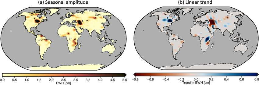
S. Deggim et al.: GRACE correction product RECOG RL01                                                                            2231

lakes will be added to the source databases or when their             are available upon request. This gives us the idealized sig-
time series will be updated, the algorithm for matching wa-           nal that GRACE would measure if it were influenced by the
ter level time series with their respective lake surface area         changing mass in the lakes/reservoirs only. For a grid-based
(as well as most of the following workflow) was automated.            evaluation (0.5◦ × 0.5◦ grid) a recomputation using Eq. (2) is
The first step for the combination was an automatically gen-          necessary to calculate the lake water storage 1TWSF (θ, λ)
erated data table with global common lake IDs. Where no               for every grid cell after filtering (Wahr et al., 1998), again up
IDs were available, matching was achieved by comparing                to degree and order 96:
names while making sure that no double naming occurred
in the input data. If that was not possible or no names were                                 96 Xn
                                                                              F        M X           2n + 1
given, matches were found using a very strict search algo-            1TWS (θ, λ) =      2
                                                                                                            · Pnm (cos θ ) (2)
                                                                                     4π R ρ n=0 m=0 1 + kn
rithm for the nearest lake shape to a given time series. If
none of the above methods was successful, the respective                                  F              F
                                                                                    · 1Cnm cos (mλ) + 1Snm sin(mλ) .

lake was dismissed and not included in the correction. In to-
tal, matches for 283 lakes/reservoirs were found for RECOG-
LR RL01 (see Fig. 2); a detailed list is provided in the Sup-         Here we included the density of water ρ (1025 kg m−3 ) to
plement (Sect. S1). The surface waterbody shapes were then            obtain a lake water storage result in metres of equivalent wa-
discretized on a fine-resolution, 0.025◦ grid to be able to cap-      ter heights (EWHs), corresponding to the input variations in
ture long but narrow reservoirs in valleys. As in our algo-           water storage from the water level time series.
rithm grid cells are only assigned to belong to a waterbody if
their midpoint lies within the lake polygon, small waterbod-          2.1.5   Results for RECOG-LR
ies would otherwise be missed completely. Multiplication
with the altimetry-derived water height resulted in water vol-        The resulting product for the lake and reservoir correc-
ume estimates for each of the grid cells. These water volumes         tion consists of two different parts, namely (1) the forward-
were subsequently distributed proportionally over a lower-            modelled lake water correction to be subtracted from the
resolution, 0.5◦ grid to save computation time in the forward         GRACE data to remove the influence of lakes/reservoirs (re-
modelling and because a 0.5◦ resolution is more than suffi-           moval approach). It is provided both on a spherical har-
cient for applications to GRACE. The resulting global grids           monic level (coefficients 1Cnm   F and 1S F ) and as a grid-
                                                                                                                  nm
of lake/reservoir-related water height anomalies for each of          ded data product (1TWSF (θ, λ) from Eq. 2). The second
the 168 months of our investigation period then entered the           part consists of (2) the altimetry-derived monthly water lev-
forward-modelling algorithm.                                          els for each 0.5◦ grid cell that can be used to re-add the mea-
                                                                      sured lake volume to its actual area (relocation approach).
2.1.4     Forward modelling                                           Figure 2 highlights each grid cell that includes surface wa-
                                                                      terbodies with data used for the correction. Note that, al-
The localized altimetry/remote-sensing-derived surface wa-            though most of the major lakes and reservoirs are covered,
ter variations have to be converted to the GRACE spatial res-         some had to be excluded from the dataset for reasons ex-
olution before they can be subtracted from monthly GRACE              plained further in Sect. 4. Figures showing an exemplary
gravity field estimates. In this forward-modelling step, the          seasonal cycle of RECOG-LR can be found in the Supple-
gridded values were expanded into spherical harmonic coef-            ment (Fig. S3), and an animation of the monthly changes
ficients up to degree (n) and order (m) 96 according to               of the lake/reservoir water storage for the full time series is
                                                                      provided in the “Video supplement” section (Deggim et al.,
                             Zπ Z2π
              R 2 kn + 1                                              2020b; https://doi.org/10.5446/48188).

    1Cnm
           =     ·                   1TWS (θ, λ)                (1)      Figure 3a shows the mean amplitudes of the seasonal vari-
    1Snm      M 2n + 1
                             0 0                                      ations of the correction for each grid cell. The most promi-
                                                                      nent features are the Caspian Sea in Asia and the Great Lakes

                               cos (mλ)
             · Pnm (cos θ ) ·              · sin(θ ) · dλ · dθ,       in North America with amplitudes of about 10 cm. However,
                                sin (mλ)
                                                                      peaks for individual months can reach as much as 30 cm
with 1Cnm and 1Snm being the spherical harmonic co-                   of TWS correction, as shown for exemplary time series in
efficients (at degree n and order m), R the radius of the             Fig. S3. Most of the other lakes and reservoirs have mean
Earth, M the mass of the Earth, kn the load Love numbers              correction amplitudes in the area of 0 to 3 cm. Figure 3b dis-
(Farrell, 1972), 1TWS(θ λ) the changes in altimetry-derived           plays the linear trend of the lake correction product. Again,
water storage in relation to colatitude θ and longitude λ,            the most distinctive features are a strong negative trend of
and Pnm the Legendre functions. Subsequently a standard               the Caspian Sea and a strong water storage increase in the
GRACE filter was applied for smoothing (DDK3; Kusche,                 Great Lakes (altimetry time series shown in Fig. S4 in the
2007; Kusche et al., 2009). The filtered coefficients are then        Supplement for comparison). Strongly visible is also a posi-
denoted by 1Cnm F and 1S F . Differently filtered corrections         tive trend (mass increase) in Lake Victoria accompanied by a
                          nm

https://doi.org/10.5194/essd-13-2227-2021                                            Earth Syst. Sci. Data, 13, 2227–2244, 2021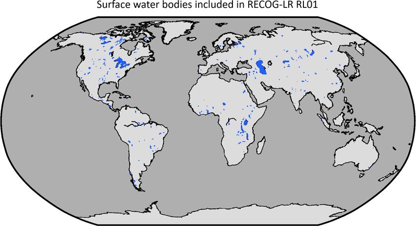
2232                                                                    S. Deggim et al.: GRACE correction product RECOG RL01

Figure 2. Overview of all 283 lakes/reservoirs in the dataset (blue areas) given on a 0.5◦ grid.

Figure 3. RECOG-LR on a global scale with its (a) mean seasonal amplitude and (b) trend.

clear mass loss in the nearby Lake Malawi. However, it also               cal harmonic coefficients have to be backward-modelled to
becomes evident that some surface waterbodies can have a                  gridded geoid changes by
rather prominent trend signal without having a strong sea-
sonality, as for example Lake Oahe in South Dakota, or ex-
hibit a strong seasonality without any long-term trend, such
as Lake Chad in Africa or Lake Guri and Tucurui Reservoir
in South America. In other surface waterbodies, such as the
                                                                                            96 X
                                                                                               n
artificial reservoir Lake Volta, the time series is dominated                               X
by a strong inter-annual signal (Ni et al., 2017), which does             1GC (θ, λ) = R              Pnm (cos θ )                  (3)
                                                                                            n=0 m=0
not show up prominently in Fig. 3 but is very much visible in
the total temporal variability shown in Fig. 5 below.                                     · (1Cnm cos (mλ) + 1Snm sin(mλ))

2.2     Earthquake correction, RECOG-EQ

2.2.1    Processing of RECOG-EQ

Different from the lake/reservoir correction, which is com-               to be able to apply the Bayesian approach provided in Einars-
puted by forward modelling using independent datasets (al-                son et al. (2010).
                                                                                            The total geoid changes for a specific
timetry/remote sensing), the earthquake correction is derived             location θi , λj can be subdivided into a bias (1GCbias ),
by fitting a parametric function to monthly GRACE data                    trend (1GCtrend ), annual- (1GCann ) and semi-annual signal
along the following processing line: in a first step, spheri-             (1GCsemiann ), S2 aliasing period of 161 d (1GCN2 ), and the

Earth Syst. Sci. Data, 13, 2227–2244, 2021                                                 https://doi.org/10.5194/essd-13-2227-2021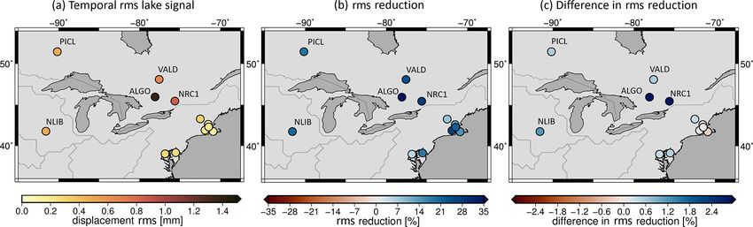
S. Deggim et al.: GRACE correction product RECOG RL01                                                                         2233

earthquake signal (1GCEQ ) as                                        2.2.2   Results for RECOG-EQ
                                                                     The correction is provided equivalently to the lake correc-

1GC θi , λj , t = 1GCbias θi , λj , t                         (4)
                                                                    tion: the dataset is processed on a global 0.5◦ grid using
                     + 1GCtrend θi , λj , t
                                                                    spherical harmonic coefficients up to degree and order 96, is
                     + 1GCann θi , λj , t                            DDK3-filtered (different filters are available upon request),

                     + 1GCsemiann θi , λj , t                        and covers the period 2003 to 2016.
                                                                        The correction only shows differences over the regions of

                     + 1GCS2 θi , λj , t + 1GCEQ θi , λj , t ,
                                                                     the 2004 Sumatra–Andaman earthquake (Fig. 4a) and the
which contains the model coefficients Cbias , Ctrend , Cann ,        2011 Tohoku earthquake (Fig. 4b) because we only corrected
φann , Csemiann , φsemiann , CS2 , and φS2 . The earthquake signal   for these two earthquakes. For the Sumatra–Andaman region
included here is described by a co-seismic and a post-seismic        the linear trends of the correction reach from about −2.7
component modelled as                                                to 1.1 cm EWH per year. Negative linear trends of down to
                                                                   −2.7 cm EWH per year can be found north of Indonesia and
1GCEQ θi , λj , t = Cvco θi , λj Htv (t)                       (5)   west of peninsular Malaysia, while positive trends are visible

                        + Cvpost θi , λj Htv (t)                     in the Indian Ocean close the coast of Sumatra. Considering
                                    t−tv (θ ,λ )
                                                 !                   Tohoku, the linear trends range from about −2.5 to 1.4. The
                                  − τ (θ ,λi )j
                        · 1−e            i j       .                 dominant negative part can be found to the west of the To-
                                                                     hoku region, while the positive parts are apparent in the Pa-
Cvco and Cvpost describe coefficients for the co- and post-          cific Ocean, southeast of Tohoku. These results suggest that
seismic component of the respective earthquake v, Htv (t) is         uncorrected TWS changes might hinder the correct analysis
the Heaviside step function at time tv , and τ is the decay          of the data for hydrological studies, because the post-seismic
rate. All coefficients are then estimated using Monte Carlo          part of the earthquake might falsely be interpreted as a linear
integration for quasi-linear models and are used to estimate         trend in the uncorrected TWS changes. This is particularly
the total earthquake signal. This signal is then removed from        relevant when the earthquake occurs at the beginning of the
the total geoid changes for each considered earthquake to            time series as is the case for the Sumatra–Andaman earth-
derive an earthquake-corrected dataset. Furthermore, we ap-          quake. The results shown here are derived from the ITSG-
plied a spatial radial Gaussian window with a radius (half           Grace2018 solutions (Kvas et al., 2019). Earthquake correc-
width) of 157 km to consider only regions that were af-              tions derived from other GRACE solutions provide similar
fected by earthquakes. The centre of the Gaussian window is          findings; for completeness they are attached in the Supple-
placed in the epicentre of the respective earthquake. Einars-        ment (Figs. S5 and S6). We do not apply geophysical for-
son’s approach is, as recommended, consecutively applied             ward modelling since these models heavily depend on dislo-
to earthquakes with a magnitude that is larger than or equal         cation parameters, fault geometry, and background rheology,
to 9.0, which is a criterion met by the Sumatra–Andaman              and parameters are typically tuned to fit seismic and GNSS
earthquake (M9.1) in December 2004 and the Tohoku earth-             measurements but do not fit observed gravity changes.
quake (M9) in March 2011. Einarsson (2011), for example,
showed that earthquakes with a magnitude larger than 9.0 are         3   Applications and validation
clearly visible in GRACE data, while earthquakes with lower
magnitude cannot always be clearly separated. For more in-           In this section we would like to show the influence and ben-
formation about the approach see Einarsson et al. (2010)             efit of the correction datasets. For this purpose, in Sect. 3.1
and Einarsson (2011). To derive TWS anomalies, the geoid             we first illustrate the impact of subtracting the two correc-
changes are forward-modelled to spherical harmonic coeffi-           tions RECOG-LR and RECOG-EQ from the GRACE time
cients similar to Eq. (1) by                                         series in terms of change in signal variability and trends.
                                                                     This includes a short discussion of the benefit of RECOG-
               Zπ Z2π                                             LR for data assimilation into hydrological models, one of
    1Cnm       1
           =             1TWS (θ, λ) · Pnm (cos θ )           (6)    the main target applications of the corrected GRACE dataset.
    1Snm      R
                  0 0
                                                                     The comparison to GNSS surface displacements (Sect. 3.2)
                                                                  not only shows the influence of the surface water correction
                 cos (mλ)
             ·              · sin(θ ) · dλ · dθ                      on geometrical surface deformations even several hundreds
                 sin (mλ)
                                                                     of kilometres around lakes/reservoirs but also represents a
and again backward-modelled to TWS changes as described              first validation of the corrected GRACE time series using in-
in Eq. (2). The final earthquake correction product, RECOG-          dependent observations. Finally, the influence of removing
EQ, is then derived by computing the difference between              earthquake signals (RECOG-EQ) for hydrological drought
the uncorrected and earthquake-corrected TWS anomalies               detection is described in Sect. 3.3.
(TWSA).

https://doi.org/10.5194/essd-13-2227-2021                                           Earth Syst. Sci. Data, 13, 2227–2244, 2021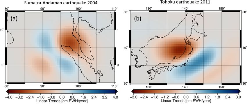
2234 S. Deggim et al.: GRACE correction product RECOG RL01
Figure 4. Linear trends (January 2003–December 2016) of TWS changes (cm EWH yr−1 ) of the earthquake correction that includes the (a)
Sumatra–Andaman earthquake from 2004 and the (b) Tohoku earthquake from 2011.
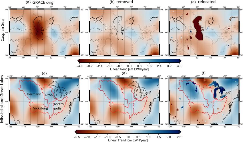
3.1 Influence of RECOG RL01 on a global GRACE time covered after subtracting the correction, should not be com-
series pletely ruled out, e.g. in the case of water transfer between
compartments as from glacier/snow to lake water (Castel-
3.1.1 Influence of lake/reservoir correction, RECOG-LR, lazzi et al., 2019).
on GRACE Figure 6 shows the influence of the lake correction on the
linear trend in the GRACE time series for two detailed exam-
We first investigate the influence of subtracting the ples; a global map can additionally be found in the Supple-
lake/reservoir correction dataset from a global GRACE time ment (Fig. S7). In the area around the Caspian Sea (Fig. 6a–
series. For this purpose, we derive gridded TWSA from the c), a very strong negative trend of around −3 cm yr−1 in
ITSG-Grace2018 (Mayer-Gürr et al., 2018; Kvas et al., 2019) the original GRACE time series (a) is almost completely re-
spherical harmonic expansion up to degree and order 96 con- moved by the lake correction (b). The relocation approach
sidering corrections for low-degree coefficients (Swenson et then restores the altimetry-derived lake water variation to
al., 2008; Cheng et al., 2011; Sun et al., 2016), glacial iso- the lake area (c). The second example shows the Mississippi
static adjustment (A et al., 2013), and applying the DDK3 Basin (Fig. 6d–f). Even though the Great Lakes are not part
filter (Kusche, 2007). of the basin, they still have an effect, particularly on subbasin
For the removal approach, we then reduce the lake cor- Alton (upstream from Alton, Illinois, USA), which is clos-
rection (Sect. 2.1.5) from the GRACE-derived TWSA grids. est to the Great Lakes. Influences of the lake variations on
For the relocation approach, we re-add the altimetry-derived the GRACE basin average of this subbasin can reach values
monthly water mass estimates. This leads to three global of up to 5 cm in TWS for some months. This example also
TWSA datasets: (1) GRACE-based only, (2) GRACE TWSA shows that a positive trend visible in the original GRACE
after removing altimetry-based lake/reservoir storage, and data can mainly be attributed to surface water change and
(3) GRACE TWS with relocated altimetry-based lake signal. can be levelled by the correction. Subtracting the lake correc-
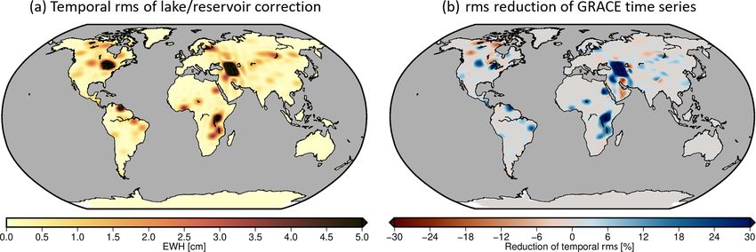
Figure 5a shows the temporal root means square (rms) of tion also reduces the positive trend partly caused by smaller
the lake correction for each grid cell. Subtracting this cor- lakes/reservoirs (e.g. Lake Oahe and Lake Sakakawea) in the
rection reduces the temporal rms variability in the GRACE Hermann subbasin in the northwest of the Mississippi.
time series (Fig. 5b) by up to 75 % around the Caspian Sea The importance of correcting the signal in the nearby
in Asia and 50 % around Lake Victoria in Africa, compared Great Lakes and the smaller lakes/reservoirs within the sub-
to the original variability in ITSG-Grace2018. Values around basins can also be detected when assimilating GRACE-
the other lakes vary between 0 and 30 % with a few negative derived TWSA into a hydrological model. The original and
values in the area south of the Caspian Sea and in Canada. the RECOG-corrected, subbasin-averaged GRACE TWSA
The latter can most likely be attributed to Gibbs oscillations of the Mississippi River basin were assimilated into the Wa-
by the bandlimited spectral representation of the data and/or ter – Global Assessment and Prognosis (WaterGAP; Döll et
to being spuriously introduced by the non-isotropic DDK3 al., 1999; Alcamo et al., 2003; Müller Schmied et al., 2014)
filter applied to the lake signals. However, the option that the hydrological model, which has a 0.5◦ × 0.5◦ grid spatial res-
lake signal was hiding another impact, which can only be re-
Earth Syst. Sci. Data, 13, 2227–2244, 2021 https://doi.org/10.5194/essd-13-2227-2021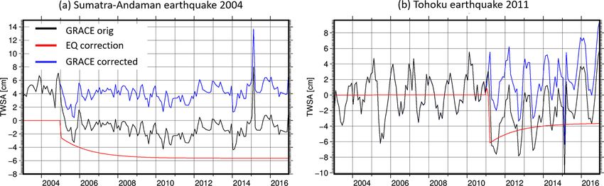
S. Deggim et al.: GRACE correction product RECOG RL01                                                                                 2235

Figure 5. Temporal root mean square (rms) of the lake/reservoir correction time series for each grid cell (a) and the relative reduction in
temporal rms when subtracting the correction (removal) from the original GRACE TWS time series (b).

Figure 6. Linear trend of GRACE TWS anomalies (January 2003–December 2016) in the Caspian Sea region (a–c) and in the Mississippi
Basin and around the Great Lakes (d–f) without any correction (a, d), after removing the influence of lakes (b, e), and after relocating the
lake signal (c, f). Please note that the Aral Sea has been excluded from RECOG-LR RL01 due to its strongly varying surface area, which is
not yet captured in the database.

olution. Our assimilation theory follows Eicker et al. (2014)           fore assimilation reduces the linear trend in the subbasin to
and Schumacher et al. (2015, 2016); for more information                0.9 mm EWH yr−1 and thus prevents the spurious trend from
see the Supplement (Sect. S8).                                          appearing in the model output. This can also be confirmed
   In the Alton subbasin, the assimilation of the original              on the grid cell level with a trend reduction in 53 % of the
GRACE observations introduces a spurious positive mass                  grid cells in the Alton subbasin, 40 % of them by more than
trend of 2.5 mm EWH yr−1 not present in the original Wa-                80 % compared with the results of assimilating the original
terGAP version. This trend is assumed to not originate from             TWSA. The strongest reductions appear in the northeastern
storage increase within the subbasin itself but to be caused            part of the basin, e.g. from 12.3 to 3.5 mm EWH yr−1 in a
by leakage due to a water storage increase in the Great Lakes           grid cell in close proximity to the Great Lakes (lat 46.25◦ ,
(see Fig. 6), particularly in the nearby Lake Superior and              long −90.25◦ ). In grid cells directly affected by lake water
Lake Michigan. Applying the RECOG correction dataset be-                storage the effect can be even larger; e.g. for Lake Sakakawea

https://doi.org/10.5194/essd-13-2227-2021                                                Earth Syst. Sci. Data, 13, 2227–2244, 2021
2236                                                               S. Deggim et al.: GRACE correction product RECOG RL01

(lat 48.25◦ , long −103.25◦ ) the trend in the assimilation re-     post-seismic relaxation afterwards, but in this case the relax-
sults changes from 493.5 to 8 mm EWH yr−1 , and the signal          ation is slowly decreasing the amount of correction. How-
rms from 2548 to 120 mm. The results reveal the importance          ever, both examples clarify that uncorrected GRACE data
of applying a lake water correction to GRACE data before            could lead to wrong conclusions about the underlying signals
data assimilation not only for areas covered by waterbod-           as the apparent trends can, for instance, hamper the identifi-
ies but also for neighbouring grid cells affected by strong         cation of drier and wetter years in the GRACE time series.
leakage-in effects.
                                                                    3.2   Validation of RECOG-LR with GNSS
3.1.2   Influence of earthquake correction, RECOG-EQ,
        on GRACE
                                                                    Global Navigation Satellite System time series contain
                                                                    signals resulting from surface mass redistribution: atmo-
This section presents the application of the earthquake cor-        spheric pressure, non-tidal oceanic loading, and hydrologi-
rection (Sect. 2.2) to the GRACE data. Linear trends for            cal changes. Vertical displacement due to hydrological load-
the period 2003 to 2016 are derived from (1) the original           ing can be predicted by calculating the elastic response of
GRACE TWSA and (2) the corrected TWSA after applying                an Earth model to the TWS changes. Previous studies have
RECOG-EQ. The correction changes the spatial pattern of             shown good agreement between modelled deformation from
the linear trend in the Sumatra–Andaman region (Fig. 7a and         GRACE TWS and vertical displacement observed by GNSS
c), and the magnitude of positive trends increases by about         (e.g. Springer et al., 2019; Tregoning et al., 2009; van Dam
0.5 cm EWH yr−1 from 4.2 to 4.7 cm EWH yr−1 . The spatial           et al., 2007), while horizontal displacements due to hydro-
extension of the positive trends in the corrected data (Fig. 7c)    logical loadings are much smaller than the vertical ones and
reaches to peninsular Malaysia. Thus, the former slightly           have been found to be systematically underpredicted and out
negative trends of about −1 cm EWH yr−1 identify a smaller          of phase (Chanard et al., 2018).
magnitude or even slightly positive values in the earthquake-          Here we use vertical displacement residuals from the
corrected dataset. The change in trends might bias the correct      ITRF2014 stacking (Altamimi et al., 2016) resulting from the
analysis of linear trends for this region.                          second reprocessing campaign (repro2) by the International
   When analysing the Tohoku earthquake results (Fig. 7b            GNSS Service (IGS) (Rebischung et al., 2016) to validate
and 7d), we also see that the magnitude and spatial pattern of      the GRACE lake/reservoir correction data product RECOG-
the trends change. In this case, the difference between orig-       LR. The station velocities and discontinuities have been care-
inal and corrected GRACE data is more obvious than in the           fully removed from the GNSS time series. To be consistent
Sumatra–Andaman region: the original dataset shows posi-            with GRACE TWS, the effects of atmospheric and non-tidal
tive linear trends of about 2 cm EWH yr−1 in the west of To-        oceanic loading are subtracted from the time series using the
hoku, while negative trends of about −2 cm EWH yr−1 can             AOD1B product (Dobslaw et al., 2017). The displacements
be found in the Pacific Ocean along the southeastern coast.         due to non-tidal oceanic and atmospheric loading are cal-
These trend signals vanish almost completely after subtract-        culated at daily epochs to be consistent with the GNSS ob-
ing the earthquake correction, confirming our assumption            servations. GRACE TWS anomalies are converted into dis-
made in Sect. 2.2.2: the post-seismic earthquake component          placements in the spatial domain using spatial convolution
was identified as linear trends in the original GRACE data          of a point mass load Green’s function (Farrell, 1972) in the
and has clearly biased the trend analysis, leading to misinter-     centre-of-figure frame using a set of high-degree load Love
pretation of the trends, especially for the Tohoku region.          numbers determined by H. Wang et al. (2012) for the Pre-
   To analyse the effect of earthquakes on TWS changes in           liminary Reference Earth Model (PREM) (Dziewonski and
more detail and over land, spatially averaged TWS anoma-            Anderson, 1981). Finally, the daily GNSS displacements are
lies are compared for peninsular Malaysia in Fig. 8a and for        averaged to monthly intervals before removing the tempo-
Japan in Fig. 8b. Additional figures showing the signal in          ral mean and linear trend from both GNSS-observed and
the epicentre of the two earthquakes are shown in the Sup-          GRACE-derived (modelled) displacements. Exemplary time
plement (Fig. S9). Regarding peninsular Malaysia, the un-           series for GNSS-observed and GRACE-modelled displace-
corrected TWSA (black) show a strong decrease in TWS                ments at different stations in the Great Lakes, Lake Victo-
changes beginning in 2004, which results from the Sumatra–          ria, and Caspian Sea regions are shown in the Supplement
Andaman earthquake. After applying the correction (blue),           (Fig. S10). Here the GNSS time series are used to assess
this strong decrease is removed. The correction (red) shows         the impact of the lake/reservoir correction on GRACE data.
nicely the co-seismic component of about −2.5 cm EWH as             To get an idea of the magnitude of its influence, we first
a jump between December 2004 and January 2005 and a fol-            show the temporal rms of the forward-modelled RECOG-
lowing post-seismic relaxation, which increases the total cor-      LR signal (Fig. 9a) for ITRF2014 GNSS sites around the
rection towards −6 cm. Similar findings can be observed for         Great Lakes. This represents the signal variability of mod-
the results for Japan and the Tohoku earthquake: the correc-        elled station displacements caused only by the surface water
tion contains a co-seismic component down to −6 cm with             variations described in RECOG-LR. The rms of the vertical

Earth Syst. Sci. Data, 13, 2227–2244, 2021                                          https://doi.org/10.5194/essd-13-2227-2021
S. Deggim et al.: GRACE correction product RECOG RL01 2237
Figure 7. Linear trends (January 2003–December 2016) of TWS changes (cm EWH yr−1 ) before and after removing earthquake signals of
the Sumatra–Andaman earthquake from 2004 (a, before; c, after) and the Tohoku earthquake from 2011 (b, before; d, after).
Figure 8. Spatially averaged GRACE TWS anomalies for the original (black) and earthquake-corrected (blue) GRACE data and its correction
(red) for (a) peninsular Malaysia (West Malaysia) and (b) Japan.
displacements amounts to up to 1.4 mm for station ALGO To investigate the agreement of observed (GNSS) and
(∼ 190 km away from the lake shore) and can reach higher GRACE-derived displacement time series, we compute the
values for other stations provided by NGL (Blewitt et al., reduction in temporal rms after subtracting the modelled
2018) (not shown), such as 2.3 mm at station BAKU close to displacements from the observed time series. For this we
the Caspian Sea and 2.5 mm at CHB5 directly at the shore of first compute the signal variability rmsGNSS of the ob-
Lake Huron. served station displacements and subsequently the variabil-
ity rmsGNSS-GRACE of the GNSS time series after subtracting
https://doi.org/10.5194/essd-13-2227-2021 Earth Syst. Sci. Data, 13, 2227–2244, 20212238 S. Deggim et al.: GRACE correction product RECOG RL01
Figure 9. Temporal rms of the vertical displacement caused by the forward-modelled lake/reservoir signal of RECOG-LR (a), reduction
of rms of GNSS time series after subtracting modelled deformation (b), and difference in rms reduction when subtracting GRACE after
removing and relocating RECOG-LR vs. using the uncorrected GRACE signal (c).
GRACE-derived station movements. The relative reduction Here it should be noted that these stations are not located
in the rms is given by the following equation: close to the shore but between 100–400 km away from the
lakes, yet they are still affected by the correction of the lake
rmsGNSS − rmsGNSS-GRACE signal. To put these numbers of up to 6 % improvement into
rmsreduction (%) = × 100. (7)
rmsGNSS perspective, a change in the Earth model used for the con-
version of TWS to deformation, which has previously been
This relative reduction in rms is shown in Fig. 9b, and it can found to be relevant for GNSS analysis (Karegar et al., 2017),
be observed that, by removing the modelled displacement has a much smaller influence. The differences in rms reduc-
based on GRACE from the GNSS time series, all stations tion using, for example, different sets of load Love num-
around the Great Lakes have their rms reduced, indicated bers amount to only < 0.4 %. Thus, from the above results,
by positive rms reductions. This means for ITRF2014 GNSS we are confident that correcting for the leakage effect of
sites around the Great Lakes we can explain some of the ob- lake/reservoir water storage in GRACE time series can have
served vertical displacement by TWS changes at most of the a considerable positive effect on the comparison of GRACE
stations, with a stronger agreement at stations closer to the and GNSS observations.
Great Lakes (ALGO and NRC1 stations).
To assess the influence of RECOG-LR on these reduc-
tions, we compute two different versions of Eq. (7): we com-
pare the rms reductions using (1) the original (unmodified) 3.3 Hydrological drought detection with earthquake
GRACE data and (2) GRACE after subtracting and relocat- correction, RECOG-EQ
ing the lake signal. The difference between these two rms re-
ductions is plotted in Fig. 9c. A positive value means that the Hydrological drought detection using GRACE data has been
RECOG-corrected GRACE signal explains a better portion applied in various studies, for example in Houborg et al.
of the observed GNSS station displacements than the uncor- (2012), Thomas et al. (2014), Zhao et al. (2017), Boergens
rected GRACE signal. All but one of the stations around the et al. (2020), and Gerdener et al. (2020a) for many regions of
Great Lakes show a positive effect of the lake correction. The the Earth. Removing the earthquake signal before the anal-
only station unimproved is located quite far from the lakes, ysis might lead to a change in the drought detection results,
directly at the coast of the ocean, and might primarily be in- which could have a significant impact on, for example, the
fluenced by oceanic leakage as discussed in van Dam, et al. decisions of policy makers. In this section, we show an exam-
(2007). The largest improvements can be observed at stations ple of the influence of the earthquake correction (Sect. 2.2)
ALGO (6.1 %) and NRC1 (4.3 %), both around 180–200 km for detecting drought events in peninsular Malaysia. To show
away from Lake Huron. In the time series plot in Fig. S10 the longer-term behaviour of droughts, the drought severity
of the Supplement this improvement is indicated by a better index using accumulation (DSIA) used in Gerdener et al.
fit of the corrected GRACE time series with the GNSS ob- (2020a) is computed. As typically done with meteorological
servations. Also for other ITRF2014 stations in the area of indicators, the observable is accumulated for a chosen pe-
large surface waterbodies we find a systematic improvement riod q (1TWS+ i,j,q ) before its computation because we refer
of the rms reduction when applying RECOG-LR. Examples it to a duration of drought. For example, if the accumulation
are stations around the Caspian Sea (NSSP: 0.2 % improve- period q is set to 3 months, the accumulated TWS changes
ment; TEHN: 0.3 % improvement) and around Lake Victoria for March 2003 will be the sum of TWS changes of January,
(NURK: 1.4 % improvement; RCMN: 2.7 % improvement). February, and March. The accumulation also serves as a run-
Earth Syst. Sci. Data, 13, 2227–2244, 2021 https://doi.org/10.5194/essd-13-2227-2021S. Deggim et al.: GRACE correction product RECOG RL01 2239
ning mean. The DSIA is then computed by also Sect. 2.1.1). More generally, we only consider surface
waterbodies that can be captured by satellite altimetry and
1TWS+ +
i,j,q − 1TWSj,q this way underestimate the impact of surface water storage
DSIAi,j,q = + , (8) in regions with a large number of small lakes and dams, e.g.
σj,q
in the US or in India.
Additionally, changes in surface water volume also affect
where 1TWS+
i,j,q is the accumulated TWS changes in year surrounding groundwater storage (and thus GRACE data) by
i and month j = 1, . . ., 12; 1TWS+ j,q is the mean monthly groundwater–surface water interactions (e.g. Bierkens and
accumulated TWS change, e.g. the mean over all Januar- Wada 2019), which have not yet been considered in our data
+
ies; and σj,q is the monthly standard deviation. Here, it is product. Steric effects caused by the thermal expansion of
used to identify hydrological drought events for an accumu- water have an influence on the altimetry-derived water levels
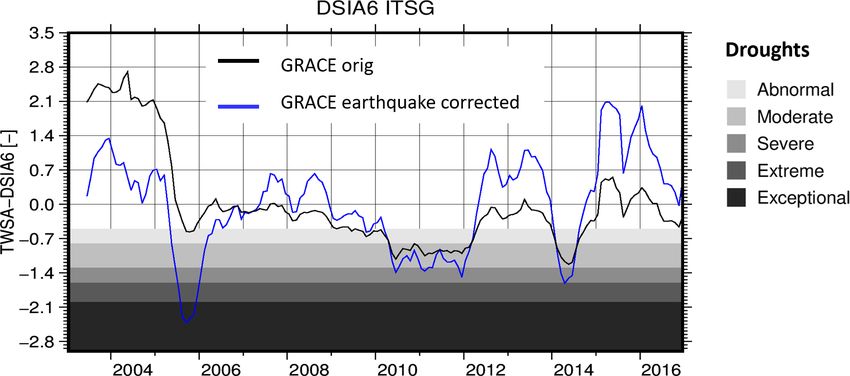
lation period of 6 months (DSIA6) over peninsular Malaysia. in large surface waterbodies, which have not been accounted
Figure 10 shows the resulting DSIA6 time series using cor- for in the conversion from water volume to mass change.
rected (blue) and uncorrected (black) TWS changes. The un- Studies only exist for very large lakes, such as the Caspian
corrected DSIA6 identifies a mainly moderate dry period in Sea, where the steric water level change was found to amount
2010 and 2011 and a severe period at the beginning of 2014. to about 1/3 of the seasonal amplitude (Chen et al., 2017;
Both periods are also identified using the corrected DSIA6 Loomis and Luthcke, 2017). We expect this to be an extreme
but with different intensity. The period 2010/11 is slightly case, with the influence on smaller waterbodies being consid-
more intense now, and the drought in 2014 is extreme (e.g. erably smaller. However, since the necessary temperature and
Tan et al., 2017). Furthermore, the corrected DSIA6 shows salinity profiles are not available on a global scale including
exceptional drought in 2005, which was not identified with smaller waterbodies, no steric correction has been included
the uncorrected DSIA6. These findings are supported by, in RECOG-LR.
for example, the EM-DAT database (EM-DAT, 2020) and
Hashim et al. (2016), who also identified a drought over
peninsular Malaysia in 2005. However, in March 2005, a 5 Code availability
second earthquake (Nias earthquake) also occurred close to
The GROOPS software toolkit has been used. It is available
the Sumatra–Andaman region with a magnitude of M8.6. As
on GitHub: https://github.com/groops-devs/groops/commit/
stated by, for example, Broerse (2014), earthquakes with a
a52631fc1817acdc4b40e1caae546254f36a2653 (last access:
lower magnitude are not always clearly visible in the data,
6 November 2020; Mayer-Gürr et al., 2020).
but it should be noticed that the Nias earthquake might still
have possible influences on the time series analysis.
6 Data availability
4 Limitations
RECOG includes (1) RECOG-LR with (1a) global gridded
As mentioned in Sect. 2.1, static lake shapes were used to time series for the given time span with the correction
determine the lake volume and subsequently the mass esti- values in total water storage for each grid cell and month,
mates in this first release of RECOG. In contrast to monthly (1b) the same values in SH coefficients of degree and order
or daily lake shapes, these are not (or much less) impacted 96, and (1c) the monthly gridded altimetry-derived water
by cloud coverage in the optical satellite images and, thus, height for the relocation approach and (2) RECOG-EQ
more reliable. This approximation works for most of the with the monthly gridded earthquake correction for TWS
lakes with shores that are not too flat. Estimated errors caused changes, containing the 2004 Sumatra–Andaman and the
by ignoring the changing surface area revealed numbers be- 2011 Tohoku earthquake. The data have been uploaded
tween 3–15 % for exemplary surface waterbodies (Semmel- to the PANGAEA database: RECOG-LR: Deggim et
roth, 2019). Extreme cases with either very flat shores and al. (2020a), https://doi.org/10.1594/PANGAEA.921851;
high water level variations or strong trends such as the Aral RECOG-EQ: Gerdener et al. (2020b),
Sea in Asia, whose surface area shrunk to a fraction of its https://doi.org/10.1594/PANGAEA.921923.
original size in the last couple of decades, have been omitted
in the correction. 7 Conclusions and outlook
Though RECOG-LR covers most of the major lakes
around the world, some are not yet implemented in the Leakage effects of surface waterbodies and non-hydrology-
dataset due to failed automatic matching between water level related mass change signals have a strong influence on water
time series and lake surface area (e.g. Lake Athabasca, see storage estimates from GRACE, complicating its use for hy-
also Sect. 2.1.3), insufficient water level time series due to drological studies and specifically for calibration and data as-
ice coverage for major parts of the year (e.g. Lake Taymyr) similation. Volume change estimates from combining satel-
or missing flyovers by altimeter satellites (e.g. Dead Sea; see lite altimetry with remote sensing information can be used to
https://doi.org/10.5194/essd-13-2227-2021 Earth Syst. Sci. Data, 13, 2227–2244, 20212240 S. Deggim et al.: GRACE correction product RECOG RL01
Figure 10. GRACE-derived TWSA DSIA6 over peninsular Malaysia (West Malaysia) shown without (black) and with (blue) earthquake
correction.
remove (or at least strongly reduce) the effect of lakes and in peninsular Malaysia, which a GRACE-based drought in-
reservoirs from the GRACE data on a global scale, with par- dicator would otherwise have missed without first correcting
ticular benefit in regions close to big lakes/reservoirs or in for the earthquake signal. Therefore, depending on the ap-
regions with many smaller lakes and reservoirs. The earth- plication at hand, we recommend applying both RECOG-LR
quake signal (co-seismic and post-seismic), which masks hy- (globally) and RECOG-EQ (especially when research is per-
drological variations in the vicinity of large earthquakes, can formed in areas that underlie large earthquakes) as a standard
be extracted directly from the GRACE time series. post-processing step for analysing GRACE data.
In this contribution, we introduced the first release of a Future improvements of the correction data product will
new global correction dataset, RECOG RL01, for removing introduce dynamic lake shapes replacing the static lake sur-
both the lake/reservoir storage (RECOG-LR) and the earth- face areas used so far, which will enable the inclusion of sur-
quake signal (RECOG-EQ) from the GRACE time series, face waterbodies with major area changes, such as the Aral
while also offering the possibility to relocate the altimetry- Sea. Alternatively, pre-processed volume change time series
derived mass change to its original surface waterbody out- of DAHITI (Schwatke et al., 2020) can be introduced for
line. lakes for which they are already provided. The GRACE time
Exemplary applications show that the correction product series continues thanks to GRACE-Follow-On, and it is thus
can reduce the signal variability (rms) of the GRACE sig- important to also provide a continuously updated surface wa-
nal by up to 75 % for the most prominent example of the terbody correction which will rely on continuously updated
Caspian Sea and that affected areas not only include the lake source data. An extension of the RECOG-LR to include fur-
areas themselves but can also extend for tens to hundreds ther surface waterbodies and a closure of existing data gaps
of kilometres around the waterbodies due to leakage. Spe- as soon as new data are added to DAHITI will easily be pos-
cial precaution has to be taken when assimilating GRACE sible thanks to a largely automated process of matching lake
data into hydrological models in the proximity of large sur- IDs in the altimetry database with corresponding lake shapes
face waterbodies. In this context, the correction product is and forward-modelling the water volume to filtered GRACE-
particularly valuable for models that do not include a sur- like TWS. Thus RECOG-LR can be updated as soon as new
face water compartment at all, but the reduction of the leak- data become available.
age effect can also make it beneficial for models that do. So far, RECOG-LR focusses on lakes and reservoirs.
For the example of the Alton subbasin of the Mississippi However, there are other forms of surface waterbodies whose
the leakage signal of the Great Lakes would cause an ar- effects on GRACE data are still disregarded and not yet cov-
tificial mass increase in the assimilated model runs of Wa- ered by any correction. An example for this are rivers, espe-
terGAP, which can be prevented by subtracting and relocat- cially river deltas of big river basins (e.g. Mississippi, Ama-
ing the surface water storage before assimilation. A valida- zon, Congo) that are highly influenced by strong seasonal
tion of the corrected GRACE signal using observed vertical variations in water flux as well as influences by tides in the
GNSS station displacements shows an improvement of the estuary. Such a correction would be especially interesting for
fit between GRACE and GNSS of up to 6 % for stations at hydrological modelling.
around 180–200 km distance from the Great Lakes. Apply- The correction data product can also be extended to cover
ing the earthquake correction allows for the determination of additional geophysical phenomena. For example, since most
several severe and one exceptionally severe drought events hydrological models do not include an explicit glacier com-
Earth Syst. Sci. Data, 13, 2227–2244, 2021 https://doi.org/10.5194/essd-13-2227-2021You can also read


