Long-term variance of heavy precipitation across central Europe using a large ensemble of regional climate model simulations - KIT
←
→
Page content transcription
If your browser does not render page correctly, please read the page content below
Earth Syst. Dynam., 11, 469–490, 2020
https://doi.org/10.5194/esd-11-469-2020
© Author(s) 2020. This work is distributed under
the Creative Commons Attribution 4.0 License.

                     Long-term variance of heavy precipitation
                   across central Europe using a large ensemble
                       of regional climate model simulations
                       Florian Ehmele, Lisa-Ann Kautz, Hendrik Feldmann, and Joaquim G. Pinto
         Institute of Meteorology and Climate Research, Department Troposphere Research (IMK-TRO), Karlsruhe
        Institute of Technology (KIT), Hermann-von-Helmholtz-Platz 1, 76344 Eggenstein-Leopoldshafen, Germany
                                  Correspondence: Florian Ehmele (florian.ehmele@kit.edu)

                                  Received: 26 August 2019 – Discussion started: 2 September 2019
                             Revised: 9 March 2020 – Accepted: 26 April 2020 – Published: 26 May 2020

       Abstract. Widespread flooding events are among the major natural hazards in central Europe. Such events are
       usually related to intensive, long-lasting precipitation over larger areas. Despite some prominent floods during the
       last three decades (e.g., 1997, 1999, 2002, and 2013), extreme floods are rare and associated with estimated long
       return periods of more than 100 years. To assess the associated risks of such extreme events, reliable statistics
       of precipitation and discharge are required. Comprehensive observations, however, are mainly available for the
       last 50–60 years or less. This shortcoming can be reduced using stochastic data sets. One possibility towards this
       aim is to consider climate model data or extended reanalyses. This study presents and discusses a validation of
       different century-long data sets, decadal hindcasts, and also predictions for the upcoming decade combined to a
       new large ensemble. Global reanalyses for the 20th century with a horizontal resolution of more than 100 km have
       been dynamically downscaled with a regional climate model (Consortium for Small-scale Modeling – CLimate
       Mode; COSMO-CLM) towards a higher resolution of 25 km. The new data sets are first filtered using a dry-day
       adjustment. Evaluation focuses on intensive widespread precipitation events and related temporal variabilities
       and trends. The presented ensemble data are within the range of observations for both statistical distributions
       and time series. The temporal evolution during the past 60 years is captured. The results reveal some long-
       term variability with phases of increased and decreased precipitation rates. The overall trend varies between the
       investigation areas but is mostly significant. The predictions for the upcoming decade show ongoing tendencies
       with increased areal precipitation. The presented regional climate model (RCM) ensemble not only allows for
       more robust statistics in general, it is also suitable for a better estimation of extreme values.

1   Introduction                                                   decreases in extreme precipitation events (Field et al., 2012).
                                                                   This is attributed to their rare occurrence, the general high
Ongoing climate change affects not only the global scale but       spatial variability of precipitation, and a lack of long-term
also impacts the regional climate. Regarding air temperature,      high-quality observations.
there is a more or less clear trend in the recent past, which         Magnitude and sign of heavy precipitation trends strongly
reveals a clear anthropogenic signal. However, various cli-        depend on various factors such as the regarded area or the
mate simulations show distinct differences for precipitation       considered time period (e.g., Easterling et al., 2000). Global
trends, especially for heavy precipitation (e.g., Moberg et al.,   tendencies towards more intense precipitation throughout the
2006; Zolina et al., 2008; Toreti et al., 2010). A review of ob-   20th century between summer and winter seasons also ac-
served variability and trends in extreme climate events states     count for precipitation trends. For example, Moberg and
that it is difficult to find significant relations between the     Jones (2005) found an increase in winter precipitation across
greenhouse-gas-enhanced climate change and increases or            central and western Europe between 1901 and 1999, while

Published by Copernicus Publications on behalf of the European Geosciences Union.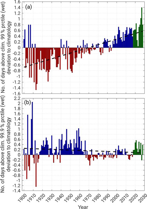
470                                                                   F. Ehmele et al.: Heavy precipitation in central Europe

Pal et al. (2004) found a decrease in summer precipitation for    underestimated. A possible reason is the decreasing number
the period 1951–2000. Dittus et al. (2016) found an increas-      and quality of observations early in the century and therefore
ing trend between 1951 and 2005 in extreme total precipi-         a lack of assimilation data. The suitability of reanalysis data
tation amounts for Europe in global climate model (GCM)           to investigate extreme precipitation for England and Wales
simulations (Coupled Model Intercomparison Project phase          was investigated by Rhodes et al. (2015). While time series
5; CMIP5). Similar trends were found in global reanalyses         of daily precipitation totals are well represented in both data
(e.g., ERA-20C; Poli et al., 2016) but not in observations. In    sets, timing errors of heavy precipitation events were identi-
contrast, Primo et al. (2019) found positive trends for two       fied as one of the major problems. Stucki et al. (2012) inves-
ground-based observational stations in Germany using ex-          tigated historical flooding events in Switzerland and indicate
treme precipitation indices.                                      that the reanalyses underestimate precipitation in Switzer-
   Model resolution is another crucial factor. The use of high-   land which may result from the insufficient representation of
resolution regional climate models (RCMs) instead of global       the alpine topography. The timing and the exact location of
data sets revealed a more detailed and orographically re-         heavy precipitation were also found to be inaccurate.
lated spatial structure of the precipitation fields and trends       As shown by van der Wiel et al. (2019) or Martel et al.
(e.g., Feldmann et al., 2013). An increase of both areal mean     (2020), large ensembles can have an added value for flood
precipitation and extremes in central Europe on the order         risk estimation and for the calculation of return periods
of 5 %–10 % was found in RCM simulations by Feldmann              of heavy precipitation. van der Wiel et al. (2019) found a
et al. (2013), which will continue with almost same magni-        clear benefit in using an ensemble approach for the esti-
tude for the next decade. Differences in precipitation trends     mation of changes in hydrological extremes including com-
also stem from varying definitions of extreme events such as      pound events compared to traditional approaches. Martel
certain thresholds, percentile-based indices, or return periods   et al. (2020) found similar results, namely a reduction in the
(e.g., Maraun et al., 2010). While most of these studies show     projected return period of 100-year annual maximum precip-
trends in daily precipitation, just a few deal with subdaily      itation with the different ensembles, albeit having different
trends. Barbero et al. (2017), for instance, compared trends      model structures and resolutions. Furthermore, it was em-
in subdaily and daily extremes. Although significant increas-     phasized that a higher resolution is advantageous to predict
ing trends were found for both time ranges, trends in daily       climate change signals over complex terrain. Other studies
extremes are better detected than in subdaily extremes.           also highlighted the improvements of using high-resolution
   Spatially extended intensive rainfall events are frequently    RCMs for the investigation of climate extremes (e.g., Feser
related to widespread flooding along the main river networks      et al., 2011; Feldmann et al., 2008, 2013; Schewe et al.,
of central Europe causing major damage on the order of sev-       2019), especially over complex terrain (e.g., Torma et al.,
eral billion euros (EUR) per event (e.g., Uhlemann et al.,        2015).
2010; Kienzler et al., 2015; Schröter et al., 2015; MunichRe,        The studies mentioned above document partly contrasting
2017). A prominent example of such an extreme and devas-          results and demonstrate the challenges arising when dealing
tating event is the flood in 2012 along the Elbe and Danube       with extreme precipitation and related phenomena. In this
rivers (Ulbrich et al., 2003a, b). Such outstanding events are    study, a set of different realizations with one RCM is used
by definition extremely rare, which makes the risk estima-        and combined to the new LAERTES-EU (LArge Ensemble
tion difficult or almost impossible due to the limited time pe-   of Regional climaTe modEl Simulations for EUrope), which
riod with available area-wide observations (e.g., Pauling and     can be used for more profound statistical analyses. The ba-
Paeth, 2007; Hirabayashi et al., 2013). However, trend anal-      sis is the global 20th Century Reanalysis (20CR) data set
yses of such extreme events and the related risks during the      (Compo et al., 2011), which was dynamically downscaled for
past and for the future are of great importance for insurance     Europe. LAERTES-EU consists of a handful of 20th century
purposes or flood protection (e.g., Merz et al., 2014; Schröter   reanalysis data sets and a large ensemble of decadal hindcast
et al., 2015; Ehmele and Kunz, 2019).                             simulations mainly for the second half of the century. Al-
   A possible way of dealing with the unsatisfactory data         though all simulations were performed with the same RCM
availability is through century-long simulations using cli-       version and setup, LAERTES-EU is a combination of differ-
mate models (e.g., Stucki et al., 2016) or stochastic ap-         ent external forcings, boundary conditions, and/or assimila-
proaches (e.g., Peleg et al., 2017; Singer et al., 2018; Ehmele   tion. Predictions for the upcoming decade will round up our
and Kunz, 2019). The currently used GCMs were found to            analysis. The investigative focus lies on daily values of inten-
be in good agreement with the available but limited observa-      sive areal precipitation which can be associated with major
tions (Fischer and Knutti, 2016). Brönnimann et al. (2013)        flood events in central Europe. As demonstrated, for exam-
and Brönnimann (2017) analyzed historical extreme events          ple, by Schröter et al. (2015), severe flood events along the
using century-long reanalysis data sets and concluded that        major river networks in central Europe are related to long-
the quality of the reanalyses strongly depends on the num-        lasting and widespread precipitation events of mainly strat-
ber and type of the assimilated observations. The investigated    iform origin with embedded convective precipitation. Typi-
historical events were reproduced, but the magnitudes were        cally, intensities do not reach the most extreme rates of the

Earth Syst. Dynam., 11, 469–490, 2020                                                https://doi.org/10.5194/esd-11-469-2020
F. Ehmele et al.: Heavy precipitation in central Europe                                                                            471

distribution but are characterized by high spatial mean val-        is a land-only data set and ocean grid points are set to a miss-
ues.                                                                ing value. Haylock et al. (2008) stated that rainfall totals in E-
   LAERTES-EU is validated in terms of coincidence with             OBS are reduced by up to almost one-third compared to the
observations regarding temporal variability, statistical dis-       raw station data at the corresponding grid cells. Regarding
tributions, and possible long-term trends. The following re-        extremes, the deviation of E-OBS is even more pronounced
search questions will be addressed.                                 (Hofstra et al., 2009). Nevertheless, both studies stated that
                                                                    the spatial mean precipitation in E-OBS is very close to other
    1. How well is extreme areal precipitation represented in       observations.
       the RCM ensemble LAERTES-EU?                                    Although E-OBS has some limitations, we use it as the
    2. What are potential benefits of LAERTES-EU compared           main reference for this study, as there is no other compara-
       to other available data sets?                                ble high-resolution daily precipitation data set available that
                                                                    covers entire Europe for a long time period. Other products
    3. Which temporal evolution and variability of extreme          like satellite data with a very limited time frame are not help-
       areal precipitation over central Europe have manifested      ful and also have limitations. There are single ground-based
       during the past?                                             observations with very long time series, but as the focus of
                                                                    this study is on intensive areal precipitation, these data are of
    4. Which tendency is expected for the upcoming decade?
                                                                    limited usefulness for validation.
A better interpretation of RCM data and a more profound                In addition to E-OBS, we compare the RCM simulations
understanding of extreme areal precipitation may have sev-          with the central European high-resolution gridded daily data
eral applications such as risk assessments. Although they are       sets (HYdrological RASter data sets; HYRAS) provided by
relevant, we do not handle the potential mechanisms behind          the German Weather Service (DWD; Rauthe et al., 2013).
temporal variance and trends as well as spatial and seasonal        HYRAS is a gridded precipitation data set with a horizontal
differences as this goes beyond the scope of this study.            resolution of up to 1 km for the time period 1951–2006 and
   This paper is structured as follows. The data sets which         covers Germany and the surrounding river catchments. The
were used in this study are introduced in Sect. 2. Section 3        HYRAS algorithm also uses ground-based measurements
sums up the methods used for the analysis and the validation.       and interpolates the point observations to the regular grid.
In Sect. 4, LAERTES-EU is validated with observations for a         For this study, the HYRAS data were first aggregated to the
reference period. The investigation of temporal variabilities       E-OBS/RCM 25 km grid. HYRAS hereafter refers to this ag-
and trends is given in Sect. 5. Finally, Sect. 6 gives a sum-       gregated 25 km data set.
mary and lists our conclusions.
                                                                    2.2   Regional climate model simulations
2     Data sets
                                                                    LAERTES-EU combines a large number of regional dynam-
Two different types of data sets are applied in this study:         ical downscaling simulations for Europe performed with a
gridded precipitation data based on observations and partly         single RCM. The used RCM is the non-hydrostatic model
century-long climate model simulations (LAERTES-EU).                of the Consortium for Small-scale Modeling (COSMO) CLi-
The observational data sets are primarily available for the         mate Mode (CLM) version 5 (CCLM5; Rockel et al., 2008),
second half of the 20th century and serve as reference data         which has a spatial resolution of 0.22◦ (≈ 25 km). The model
for the validation of the ensemble. Furthermore, we compare         covers the European domain of the Coordinated Downscal-
LAERTES-EU with the forcing global model and also with              ing Experiment (EURO-CORDEX)1 (Jacob et al., 2014).
the global 20CR data set (Compo et al., 2011), which were           Overall, the simulations use the same domain, model ver-
used as initial data for some of the simulations.                   sion, and setup, which was adapted from EURO-CORDEX
                                                                    (Kotlarski et al., 2014). According to Feldmann et al. (2008),
2.1    Observations                                                 a dry-day correction is important as climate models tend to
                                                                    overestimate the number of wet days with low intensities be-
The European observational data set (E-OBS) version 17 in-          low 0.1 mm, known as the drizzle effect (Berg et al., 2012).
cluding daily precipitation (Haylock et al., 2008; van den          In order to reduce this typical bias, a dry-day adjustment was
Besselaar et al., 2011) is a gridded data set with a horizon-       first applied to LAERTES-EU. The E-OBS data were used
tal resolution of 0.22◦ (≈ 25 km) covering the years 1950           for this correction, as they have the same spatial extension
to 2017. This version shows some improvements towards               and resolution as the CCLM simulations. All simulations are
older versions, since updated algorithms and new stations           performed within the BMBF (Federal Ministry of Education
have been included in some areas (e.g., for Poland). The E-         and Research of Germany) MiKlip II 2 project (Marotzke
OBS algorithm interpolates observations from weather sta-
tions to a regular grid using geostatistical methods (e.g., Jour-      1 http://www.euro-cordex.net (last access: 20 May 2020).
nel and Huijbregts, 1978; Goovaerts, 2000). Note that E-OBS            2 https://www.fona-miklip.de/ (last access: 20 May 2020).

https://doi.org/10.5194/esd-11-469-2020                                                 Earth Syst. Dynam., 11, 469–490, 2020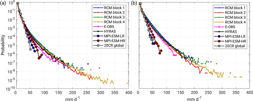
472                                                                     F. Ehmele et al.: Heavy precipitation in central Europe

et al., 2016) to create and test a decadal prediction system        ditional simulations cover the period 1960–2005 (46 years
including a regional downscaling component for Europe.              each).
   For all downscaling simulations, the boundary conditions            Data blocks 2 and 4 consist of initialized decadal simula-
were derived from the Max Planck Institute of Meteorology           tions (type III). The starting conditions are derived from an
coupled Earth System Model (MPI-ESM). This global model             observed state (Müller et al., 2012; Marotzke et al., 2016).
consists of an atmospheric component (ECHAM6) (Stevens              For each starting year, an ensemble of decadal simulations is
et al., 2013), an ocean component (MPI-OM) (Jungclaus               generated and then, the initialization point is shifted by 1 year
et al., 2013), and a land-surface model (JSBACH) (Hage-             (e.g., 1961–1970, 1962–1971, and so on). Due to the overlap,
mann et al., 2013).                                                 a specific calendar year may be covered by several decadal
   LAERTES-EU is divided into four different data blocks            hindcasts with different starting years. These decadal hind-
(Table 1) depending on the setup of the forcing MPI-ESM             and forecasts thus represent the current state of the major
ensemble simulations. The differences between the four data         modes of climate variability compared to the so-called unini-
blocks stem from the setup, external forcing, and initializa-       tialized historical simulations (data block 3). The downscal-
tion of the MPI-ESM simulations. Data blocks 1 and 2 of             ing procedure, the skill, and the added value are described
the RCM ensemble (compare Table 1) obtained the boundary            in Mieruch et al. (2014), Feldmann et al. (2019), and Reyers
values from the MPI-ESM-LR simulations using a T63 res-             et al. (2019).
olution and 47 vertical layers. Data blocks 3 and 4 used the           In data block 2, the starting conditions of the three decadal
MPI-ESM-HR version (Müller et al., 2018) as their driving           hindcast members with MPI-ESM-LR are derived from the
model. In this version, the horizontal resolution is T127 and       assimilation experiments in data block 1. The starting years
95 vertical layers are applied. Three types of forcing ensem-       of the CCLM downscaling range from 1910 to 2009. This
bles can be distinguished:                                          means the last simulated year is 2019.
                                                                       Data block 4 consists of two parts. Both of them use the
  i. MPI-ESM assimilates reanalysis data for long-term              MPI-ESM-HR version. The so-called preop-ensemble has
     simulations (data block 1);                                    five members. The external climate forcing is derived from
                                                                    CMIP5. The starting years range from 1960 to 2016 (last
 ii. long-term historical-type simulations, according to the        simulated year is 2026). The so-called dcppA-hindcast en-
     CMIP5 specifications (data block 3; Taylor et al., 2012);      semble has 10 members and uses the external forcing for
     and                                                            CMIP6 (Eyring et al., 2016). The global simulations are
                                                                    a contribution to the Decadal Climate Prediction Project
 iii. initialized decadal (10-year) hind- and forecast simula-
                                                                    of CMIP6 (DCPP; Boer et al., 2016). The starting years
      tions (data blocks 2 and 4).
                                                                    are 1960 to 2018 (last simulated year is 2028).
   In data block 1, the first type (I) is applied. Here, the 20CR      In total, LAERTES-EU consists of 1183 simulation runs
data (Compo et al., 2011) are assimilated into the MPI-ESM-         (sample size) with approximately 12 500 simulated years.
LR (Müller et al., 2014). The 20CR data set has a spatial res-      The number of ensemble members for a specific year varies
olution of approximately 2◦ (T62) and was generated using           from six at the beginning of the century to a maximum of
the Global Forecast System (GFS; Kanamitsu et al., 1991;            188 members between 1970 and 2000 (see Fig. S1 in the
Moorthi et al., 2001) of the National Centers for Environ-          Supplement). The simulations in all four data blocks are af-
mental Prediction (NCEP)3 . It used a 56-member ensem-              fected by the observed external climate forcing, but they dif-
ble Kalman filter approach to assimilate surface pressure,          fer with respect to the representation of the observed climate
monthly sea surface temperature, and sea-ice observations.          variability; whereas data block 1 uses assimilated 20CR data,
Three of the 20CR members are assimilated into MPI-ESM              data blocks 2 and 4 contain initialized hindcasts, which to
to provide long-term (110 years each) climate reconstruction        some degree follow the observed low-frequency variability,
simulations over the period 1900–2009 (Müller et al., 2014).        and data block 3 only uses the external forcing information.
Afterwards, a downscaling with CCLM uses these global               Nonetheless, the four groups of downscaling simulations can
simulations as boundary conditions (e.g., Primo et al., 2019).      be grouped into a large ensemble, since the regional simula-
   Data block 3 consists of the second type (II), where five so-    tions were all performed with the same setup of the RCM.
called historical simulations of MPI-ESM-HR with CMIP5              Despite the same initial conditions and model setup, the tem-
observed natural and anthropogenic external climate forc-           poral evolution of the day-to-day weather is (statistically) in-
ing (Taylor et al., 2012) are used as boundary conditions for       dependent between the members after a few weeks. This is
CCLM. The ensemble was generated by starting the MPI-               an advantage, since the data set is homogeneous over time
ESM from arbitrary dates in a pre-industrial control simula-        but also covers uncertainties in the observations including
tion (Müller et al., 2014). Three of the five CCLM members          unknown and not-yet-observed events. The validity of this
cover the period 1900–2005 (106 years each). The two ad-            combination approach is tested within Sect. 4.

   3 http://www.ncep.noaa.gov/ (last access: 20 May 2020).

Earth Syst. Dynam., 11, 469–490, 2020                                                  https://doi.org/10.5194/esd-11-469-2020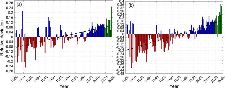
F. Ehmele et al.: Heavy precipitation in central Europe                                                                            473

Table 1. Overview of the RCM ensemble LAERTES-EU with the name of the simulation within the MiKlip project, the classification into
data blocks, the underlaying setup (experiment), the covered time period, and the number of simulation years; XX stands for the ensemble
number and YYYY stands for the initialization year.

    Name                   Block    Experiment                           Period      Years     Comment
    as20ncepXX               1      20CR via MPI-ESM-LR                1900–2009       330     3 members of 110 years each
    decXXoYYYY               2      MPI-ESM-LR DROUGHTCLIP             1911–2019     3000      3 members with 100 decades each
                                                                                               run 1–3 each with 106 years,
    historical_rXi1p1-HR     3      MPI-ESM-HR HISTORICAL              1900–2005       410
                                                                                               run 4–5 each with 46 years (1960–2005)
    preop                    4      MPI-ESM-HR CMIP5                   1961–2026     2850      5 members with 57 decades each
    dcppA-hindcast           4      MPI-ESM-HR CMIP6                   1961–2028     5900      10 members with 59 decades each

3     Methods                                                         values |1Cr | over the entire precipitation range as defined by
                                                                      Déqué (2012) or Wahl et al. (2017). The better both density
The ability of LAERTES-EU to simulate realistic precipita-            functions coincide, the lower the value of Lr . According to
tion amounts and distribution is an important requirement.            Eq. (A2), Lr is always positive. The ensemble mean is given
Moreover, temporal variability and possible trends should             by L (Eq. A3).
also be well represented for trustworthy data sets. The meth-            The internal variability of LAERTES-EU on different time
ods were applied to different investigation areas and time pe-        intervals is compared to that of the observations. Given that
riods. Equations and additional information can be found in           the focus of this study is on intensive widespread precipita-
Appendix A–C. As the focus of this study is intensive areal           tion, this analysis is performed using spatial mean precipita-
precipitation, we concentrate on high percentiles of spatially        tion amounts averaged over the investigation areas. First, the
aggregated daily rainfall totals, namely 99 %, and 99.9 %.            time series of daily spatial means are aggregated over differ-
The percentiles are based on wet days only. First, a spatial          ent intervals, namely monthly, seasonal, and yearly precipi-
aggregation of daily precipitation values was applied. After-         tation sums, as well as 5-, 10-, or 30-year running means. In
wards, the percentiles of these areal precipitation were cal-         a second step, the standard deviation of a gamma distribu-
culated for each year separately. In all data sets, ocean grid        tion σ0 is calculated for each of these interval series (see Ap-
cells were set to a missing value and therefore neglected.            pendix A; Eq. A4), for every single member of LAERTES-
                                                                      EU, and for the observations. Finally, the ensemble mean of
3.1    Validation methods                                             the four data blocks and of the complete ensemble is built.
                                                                      This method enables the analysis of how well the internal
LAERTES-EU is analyzed and validated using various meth-              variability on different timescales is captured by LAERTES-
ods. The intensity spectrum gives the statistical probability         EU.
of each precipitation amount by taking into account all grid             The quantile–quantile (Q–Q) plot compares the simulated
points and all time steps within the investigation area and           distribution with the observed one using different percentiles
without any aggregation. Therefore, the range of occurred             of daily spatial mean precipitation. The Q–Q distributions
values is divided into evenly spaced histogram classes, which         are used to calculate the coefficient of determination R 2 with
then are normalized with the total sample size. The result-           R being the Pearson correlation coefficient (Eq. A5).
ing intensity–probability curve (IPC) is a good indicator of             The added value of the ensemble size is analyzed by us-
whether the model is capable to simulate realistic precipita-         ing the signal-to-noise ratio (S2N) (Eq. A6). Therefore, we
tion intensity distributions.                                         determine a Gumbel distribution (cf. Appendix A) for dif-
   As an extension to the IPCs, the linear error in probabil-         ferent sample sizes and the corresponding 90 % confidence
ity space L (cf. Eqs. A1–A3) is analyzed (e.g., Ward and              interval. The S2N is then the ratio of the return value of the
Folland, 1991; Potts et al., 1996). Therefore, empirical cu-          Gumbel distribution divided by the 90 % confidence interval
mulative density functions (ECDFs) are calculated for each            (Früh et al., 2010).
simulation run and for the observations. The data basis is the
same as for the IPCs. The value 1Cr (Eq. A1) is defined as            3.2   Decadal variability and trend analysis
the difference between the ECDF of a model run r and that of
the observation (difference of probabilities) up to a specific        For the analysis of the temporal evolution of heavy precip-
precipitation intensity. It is therefore a measure for the over-      itation, we use time series of different percentiles of spa-
or underestimation of the model. Using 1Cr , the linear error         tial mean precipitation and quantities introduced and recom-
in probability space (Lr ; Eq. A2) is the mean of the absolute        mended by the Expert Team on Climate Change Detection

https://doi.org/10.5194/esd-11-469-2020                                                      Earth Syst. Dynam., 11, 469–490, 2020
474 F. Ehmele et al.: Heavy precipitation in central Europe
The data sets are investigated on different time peri-
ods (TPs): TP1 covers the past from 1900 to 2017, which
is divided into a subperiod (TP1b) only containing the pe-
riod 1951 to 2006, with both observations (E-OBS and
HYRAS) being available. TP2 is used for the predictions
from 2018 to 2028. Note that the simulations were performed
within the MiKlip project back in 2018 (using observations
until 2017), which is the reason why the prediction period
starts in 2018.
For climatological aspects, we use the time period
of 1961–1990, hereafter referred to as climTP. A couple of
studies (e.g., Cahill et al., 2015; Folland et al., 2018) showed
that the climate change signal for global mean temperature
significantly increased since the early 1980s. Therefore, us-
ing the time period of 1981–2010 as reference would possi-
bly include a strong changing signal to the analysis. Using
1961–1990 reduces the influence of these effects, as this pe-
Figure 1. Topographic map of Europe at model resolution 0.22◦
(in meters above mean sea level; m a.m.s.l.) with the PRUDENCE riod shows more stable conditions to a certain degree. This
regions Mid-Europe (ME; dark red box) and the Alps (AL; gray also permits more room for the interpretation of the future
box), state borders (black contours), and the HYRAS area (light red predictions.
contour). Ocean grid cells are set to a missing value.
4 Validation of the RCM ensemble
and Indices (ETCCDI; Karl et al., 1999; Peterson, 2005). In the following, the above-described methods are applied
Currently, 27 indices for temperature and precipitation are in order to validate LAERTES-EU concerning its represen-
defined by the ETCCDI. These indices can be used from tativeness with observations. With this aim, data for the in-
local to global scales. Additionally, they combine extremes vestigation period TP1b are used, and the boxes ME and AL
with a mean climatological state (Zwiers et al., 2013). In (cf. Fig. 1) are limited to the HYRAS area (ME∗ and AL∗ ).
this study, we use the two indices (R95pTOT and R99pTOT;
Eqs. B1 and B2), which indicate the amount of precipitation
4.1 Statistical distributions and frequencies
above the 95th or 99th percentile, respectively.
In terms of trend analysis, a Mann–Kendall test (Mann, The IPCs give the range of simulated (observed) precipita-
1945; Kendall, 1955) is performed with related significance tion intensities at any grid point within the investigation area
investigations (Appendix C). Regarding possible oscilla- and its corresponding probability (Fig. 2). For both investi-
tions, the complete time series is split into subseries with gation areas, the IPCs reveal a distinct added value of the
a minimum length of 10 years and up to 130 years (trend RCM compared to the global model. Due to the coarse res-
matrix). The Mann–Kendall test is applied to each of these olution, intensities greater than approximately 100 mm d−1
subseries. are not found in the GCMs, which underestimate by a large
degree the probability of the high intensities. The same ap-
3.3 Investigation areas and time periods plies for the global reanalysis 20CR. On the other hand, the
RCM tends to overestimate the probability for precipitation
The focus of this study is central Europe, implying the coun- intensities above a threshold of approximately 50 mm d−1
tries Germany, Switzerland, the Netherlands, Belgium, Lux- but covers the entire range of values as the observations. The
embourg, and parts of France, Poland, Austria, the Czech wider range of intensities at the upper tail of the distribution
Republic, and Italy. Following Christensen and Christensen may include possibly not-yet-observed events.
(2007), these countries are mostly coincident with two of For ME∗ , the IPCs of the RCM are close to HYRAS, but
the areas defined in the PRUDENCE (prediction of regional there is a systematic difference between HYRAS and E-OBS
scenarios and uncertainties for defining European climate (Fig. 2a). As already mentioned by Haylock et al. (2008),
change risks and effects) project, namely the PRUDENCE E-OBS has a certain negative bias up to −30 % when using
regions (PRs) Mid-Europe (ME) and the Alps (AL; Fig. 1). grid-point-based quantities. The given deviation of HYRAS
Although these boxes contain both land and ocean, the latter and E-OBS is within this range. Similar results can be found
was set to a missing value and neglected. During validation, for AL∗ (Fig. 2b). The differences between the RCM simula-
ME and AL were reduced to the HYRAS grid cells lying tions and the observations at a given probability are slightly
within the corresponding box, hereafter referred to as ME∗ less than those for ME∗ . For both areas, the range of sim-
and AL∗ . ulated values is much higher (up to 400 mm d−1 ). Naturally,
Earth Syst. Dynam., 11, 469–490, 2020 https://doi.org/10.5194/esd-11-469-2020F. Ehmele et al.: Heavy precipitation in central Europe 475 Figure 2. Intensity–probability curves (IPCs) of daily rainfall totals of the RCM simulations (dry-day adjusted), observations (E-OBS and HYRAS), GCM simulations (forcing MPI-ESM data at two resolutions – LR and HR), and global reanalysis data (20CR) for (a) Mid- Europe (ME∗ ) and (b) the Alps (AL∗ ), both limited to the HYRAS area during the investigation period TP1b (1951–2006). For the IPCs, every grid cell value at every time step was taken into account without any aggregation. higher intensities are more likely in the mountainous AL∗ re- LAERTES-EU and the observations can be an indicator of a gion. possibly systematic bias in this region. In contrast to the grid-point-based IPCs, Fig. 3 shows The Q–Q plots of daily spatial mean precipitation fields the mean standard deviation of a gamma distribution for both investigation areas are shown in Fig. S2. Gener- (cf. Sect. 3.1 and Appendix A) for the time series of spa- ally speaking, the distribution of the RCM is similar to those tial mean precipitation amounts aggregated over different of the observations, at least to E-OBS, with little deviations time intervals. For both areas, there is an expectable con- from the optimum (diagonal line) for most of the spectrum tinuous decrease of internal variability towards longer peri- and differences at around 10 % for the upper part of the distri- ods for all data sets/data blocks. For ME∗ , LAERTES-EU bution. In comparison to HYRAS, the maximum deviation is is in good agreement with both observations at least up to higher at around 20 %. For AL∗ , the differences between the a yearly perspective. For longer time periods, data block 1 RCM and HYRAS are larger than for ME∗ (Fig. S2). Even shows a slightly different behavior compared to the other though HYRAS was aggregated to the E-OBS/RCM grid, data blocks and observations. Nevertheless, data blocks 2–4 the more pronounced differences especially for the extremes and the ensemble mean continue to match with the observa- might be a result of the higher resolution of the HYRAS data, tions up to the 10-year running mean. Note that it is not pos- which, in particular, is of greater relevance in the mountain- sible to estimate the 30-year running mean for the decadal ous region of AL∗ . simulations of data blocks 2 and 4 given the data availability. The findings of Fig. S2 are confirmed by the determination For data block 3, only an external climate forcing was used, coefficients R 2 (Table 2). For both E-OBS and HYRAS, the meaning these so-called historicals are free runs in terms of coefficient is very high with R 2 > 0.98. There is a slightly daily weather evolution. Therefore, it is not expected that the higher R 2 for E-OBS than for HYRAS, which is an artificial multi-decadal variability is in phase to the observed circula- effect of the data resolution. The region AL∗ shows a min- tion after a certain time, which can be a reason for slightly imal higher skill compared to ME∗ in E-OBS and slightly higher differences of data block 3 compared to the observa- lower values in HYRAS. Table 2 also reveals higher correla- tions at the longest timescale. Furthermore, note that the re- tions of the CCLM simulations driven by the high-resolution sults of Fig. 3 do not indicate a perfect match of LAERTES- MPI-ESM-HR data compared to those driven by the lower- EU in terms of absolute values, but rather that the internal resolved MPI-ESM-LR data. Even though this seems to be variability (spread) of spatial mean precipitation totals is well systematic, the differences are marginal. captured. For the mountainous AL∗ region, the internal vari- Table 2 also contains the mean linear error in probabil- ability is higher and all data blocks have a higher standard ity space L for the different data blocks. Again, the differ- deviation at all time intervals. This means that the spread ences between the data blocks are marginal with all cases of simulated precipitation amounts is increased compared to being close to L = 0, which indicates good agreement of that of the observation. A possible reason for this difference LAERTES-EU with observations. In contrast to R 2 , L has can emerge from sparse measurements in that region consid- lower values for the simulations driven by MPI-ESM-LR. ered for both E-OBS and HYRAS, especially for long-term For all data blocks, L is considerably higher for the moun- observations. The more or less constant difference between tainous AL∗ region. Note that both quantities being close to https://doi.org/10.5194/esd-11-469-2020 Earth Syst. Dynam., 11, 469–490, 2020
476                                                                           F. Ehmele et al.: Heavy precipitation in central Europe

Figure 3. Mean standard deviation σ0 in mm (mean over data blocks) of spatially averaged precipitation aggregated over different time
intervals: daily (day), monthly (month), seasonal (seas), yearly (years), and 5-/10-/30-year running mean (5 yr/10 yr/30 yr) for (a) ME∗ and
(b) AL∗ (TP1b; 1951–2006). The four data blocks of LAERTES-EU are considered separately; RCM mean stands for the complete ensemble
mean (gray). The results for E-OBS and HYRAS are given in black and magenta. Note that it is not possible to estimate the 30-year values
for the decadals of data blocks 2 and 4.

Table 2. Coefficients of determination R 2 (top number) for the         tional data sets have a high year-to-year variability with sim-
quantile–quantile contemplation of Fig. S2 and linear error in prob-    ilar shape. The ensemble mean value of LAERTES-EU is
ability space L (bottom number) between the RCM and both ob-            higher, with a relative deviation of 1 %–10 % (TP1b average
servations (E-OBS and HYRAS) for Mid-Europe (ME∗ ) and the              is 7 %). The spread of both observational data sets is cov-
Alps (AL∗ ), always using HYRAS grid cells only. Both quantities        ered by the ensemble spread (minimum to maximum values)
are based on daily spatial mean precipitation amounts.                  of LAERTES-EU except for few extreme peaks (e.g., 1985).
                                                                        In AL∗ , the E-OBS mean is about 5 % higher than HYRAS
      RCM                  E-OB                  HYRAS                  but both time series have again a similar shape (Fig. S3).
                      ME∗       AL∗           ME∗        AL∗            The ensemble mean again is higher with relative deviations
                                                                        of 12 %–23 % (16 % on average) to E-OBS and 18 %–29 %
                     0.9914    0.9924        0.9876    0.9835
      Data block 1                                                      (21 % on average) to HYRAS. The ensemble spread also cov-
                     0.0016    0.0058        0.0027    0.0080
                                                                        ers the observed variability.
                     0.9914    0.9925        0.9878    0.9848              Regarding more extreme values, namely the 99.9th per-
      Data block 2
                     0.0009    0.0037        0.0021    0.0058           centile, similar results can be found (Figs. S4 and S5). Again,
                     0.9963    0.9976        0.9936    0.9930           E-OBS and HYRAS show a similar behavior for both areas
      Data block 3                                                      with mean value differences of less than 1 %. The ensem-
                     0.0017    0.0062        0.0029    0.0083
                                                                        ble mean shows a mostly positive bias with deviations of less
                     0.9966    0.9981        0.9943    0.9938
      Data block 4                                                      than 10 % (6 % on average during TP1b) compared to E-OBS
                     0.0011    0.0038        0.0023    0.0059
                                                                        for ME∗ and 6 %–18 % (average of 10 %) for AL∗ . Further-
                                                                        more, there is a distinctly higher spread and variability of the
                                                                        99.9 % for both the observations and LAERTES-EU. Except
their optimum values does not indicate a perfect model. It              for a few peaks, LAERTES-EU covers the spread of the ob-
rather means that the overall statistics regarding the entire           servations.
range of intensities to a high degree coincide with the obser-
vations.
                                                                        4.3    Added value of the sample size

4.2    Time series
                                                                        In order to demonstrate the added value of the presented
                                                                        LAERTES-EU, we use the S2N (Eq. A6) for different sam-
Besides overall statistics, other properties of LAERTES-EU              ple sizes and return periods (cf. Appendix A). Sample size, in
like the temporal variability should cover the range of ob-             this case, means the number of simulation runs. Note that the
servations as well. Therefore, we analyze the time series of            simulations vary in length (number of years) with a minimum
yearly values of different percentiles of the spatial mean pre-         length of 10 years and a maximum of 110 years. In order to
cipitation for the investigation areas. In Fig. 4, the time se-         reduce the influence of the sample length on the results, the
ries of the 99th percentile for ME∗ is shown. Both observa-             single simulation runs of LAERTES-EU were randomly con-

Earth Syst. Dynam., 11, 469–490, 2020                                                       https://doi.org/10.5194/esd-11-469-2020
F. Ehmele et al.: Heavy precipitation in central Europe 477
Figure 4. Time series of the yearly 99th percentile (wet days and
HYRAS area only) of daily spatial mean precipitation values for
Mid-Europe (ME∗ ) during TP1b (1951–2006) of the LAERTES-
EU ensemble mean (black), the ensemble spread (minimum to max-
imum; gray), E-OBS (red), and HYRAS (blue). The dotted lines
symbolize the mean values of the observations throughout TP1b.
catenated using a 100-fold permutation. Observations have
a sample size of 1. Again, S2N is calculated for daily spa-
tial mean precipitation amounts during TP1b only using the
HYRAS area.
For both ME∗ and AL∗ , S2N steadily increases with sam-
ple size for all calculated return values, indicating a more Figure 5. S2N ratio for different return periods T (colored lines)
statistically robust estimate of the return values (Fig. 5). Fur- of daily spatial mean precipitation dependent on the sample size for
thermore, the S2N is lower for higher return periods which is (a) ME∗ and (b) AL∗ . The LAERTES-EU members were randomly
a result of the increasing uncertainty of the best estimate due stringed together permuting the order a hundred times. The shown
to fewer or even no data points for very high return periods. S2N is the mean of this permutation.
However, S2N also increases with sample size for the very
high return periods. The robustness of a 2-year return value
estimate of a sample of size 1 is about the same as the 1000- namely medians, interquartile ranges, and upper whiskers,
year estimate for a sample of size 20. This means that even only small variance can be found between the different
for extremes, which have not been observed yet, some robust decades, which means that there is almost no change for
statistical analysis can be carried out. the majority of the precipitation amounts. Nevertheless, a
marked positive trend for the uppermost extremes of the dis-
5 Long-term variability and trends tributions appears with maximum values around 18 mm d−1
at the beginning of the 20th century and about 24 mm d−1
The temporal evolution and variability of extreme precipita- in the 21st century. The distribution for the upcoming
tion throughout the past time period (TP1; 1900–2017) and decade (2020–2028) shows only small differences to that of
also for the predictions (TP2; 2018–2028) are evaluated in the present decade (since 2010), with an almost equal median
this section. Besides time series of percentiles, we use cli- and interquartile range but slightly higher maximum values
mate change indices and statistical distributions. In this sec- (Fig. 6, green boxplot). Note that the decade of 2010–2019
tion, all land grid cells within the investigation areas ME and contains the years 2018 and 2019 from the predictions, and
AL are used for calculating the daily areal mean precipitation that the last “decade” 2020–2028 is shorter with 9 years.
amounts. The boxplot for AL is shown in Fig. S6 and illustrates that
not only the high percentiles reveal a decrease in the mid-
5.1 Precipitation distributions
dle of the century, but the entire distribution is shifted to-
wards lower values. Nevertheless, there is no clear tendency
Figure 6 shows the evolution of the distribution of areal for the maximum values. For the upcoming decade, the dis-
mean precipitation throughout TP1 and TP2 by treating tribution is similar to that of the present decade in the case
each decade independently. For the core of the distributions, of the median and the upper part of the distribution (Fig. S6,
https://doi.org/10.5194/esd-11-469-2020 Earth Syst. Dynam., 11, 469–490, 2020478 F. Ehmele et al.: Heavy precipitation in central Europe
Table 3. Overall trend of daily spatial mean precipitation during
TP1 and TP2 (1900–2028) using a linear regression of the yearly
series of the 99th and 99.9th percentile (Pct; wet days only) for ME
and AL. Given are absolute values and the relative changes (RCs)
compared to the climatological mean (climTP; 1961–1990) for the
ensemble minimum (min), the ensemble mean, and the ensemble
maximum (max) percentile values within LAERTES-EU, and the
related significance (p value; α = 0.05).
Area Pct Variable Trend RC climTP pα
(mm) (%) (mm)
min −0.4 −4.6 7.8 0.9387
ME 99 mean 0.8 7.8 10.3 1.0000
max 2.6 19.0 13.9 1.0000
min −1.0 −10.9 9.0 0.9974
Figure 6. Boxplot of the distribution of daily spatial mean precipi- ME 99.9 mean 1.1 8.4 13.5 1.0000
tation values (including dry days) for ME. Each decade was consid- max 6.7 31.0 21.6 1.0000
ered separately. The centerline of a box marks the median; the lower
and upper ends of the box mark the 25th and 75th percentiles (in- min −2.6 −17.1 15.4 1.0000
terquartile range); the whiskers represent approximately the 99.9th AL 99 mean 0.1 0.4 21.0 0.7208
percentile; the prediction part is marked in green. max 5.4 18.9 28.4 1.0000
min −4.3 −23.9 17.8 1.0000
AL 99.9 mean −0.0 −0.0 27.3 0.0000
green boxplot). The interquartile range is reduced due to a max 9.0 20.0 44.7 1.0000
increased lower boundary of the boxplot.
5.2 Temporal evolution of yearly percentiles
5.2.1 Overview
The overall trend during TP1 and TP2 using a linear regres-
sion for both areas and percentiles is given in Table 3. While
the ensemble mean shows a significant positive trend for ME
for both percentiles, a small but significant negative trend can
be found for the 99th percentile of AL, while there is almost
no change in the 99.9th percentile of AL. In all cases, the
ensemble spread increases due to both a decrease of the min-
imum values and an increase of the maximum values both
being highly significant. The change of the maximums is
stronger than the reduction of the minimums and more pro-
nounced in AL than in ME.
Analogous to Table 3, we analyze the trend for TP1b only
(Table S1 in the Supplement). The tendencies are the same Figure 7. Time series of the yearly 99th percentile of daily spatial
for all cases but less pronounced, except for the mean 99.9 % mean precipitation (wet days only) for Mid-Europe (ME; land only)
of AL where the negative trend during TP1b is slightly of the LAERTES-EU ensemble mean (solid line), and the ensem-
stronger than for the whole time series. ble spread (minimum to maximum; dots and shaded area) during
Figure 7 shows the temporal evolution of the 99th per- TP1 (1900–2017; black/gray) and TP2 (2018–2028; reddish).
centile during the 20th and the beginning of the 21st century
for the whole LAERTES-EU. As given in Table 3, the lower
boundary changes are small, while there is a visible positive Some differences emerge for AL (Fig. S7). At first, there
trend of the ensemble mean and the upper boundary of the is a distinct decrease of the ensemble mean between 1960
ensemble spread. Note that the larger spread from the 1960s and 1970, which might be revealed from the rising number
onwards might be artificial due to the decisively larger num- of members. As the ensemble matches well with the obser-
ber of members of data block 4. Nevertheless, there is a clear vations, we presume an overestimation of precipitation in the
consistency in the time series for ME. first half of the 20th century in that region, which could be
a result of missing data for the applied dry-day correction.
Due to the more complex terrain, the structure of the precip-
Earth Syst. Dynam., 11, 469–490, 2020 https://doi.org/10.5194/esd-11-469-2020F. Ehmele et al.: Heavy precipitation in central Europe 479
Table 4. Climatological mean (climTP; 1961–1990) of days per
year exceeding the 99th and 99.9th percentiles (Pct; wet days only)
for ME and AL, linear regression (LR) and relative change (RC)
compared to climTP for different TPs, and related significance
(p value; α = 0.05).
Area Pct climTP TP LR RC pα
ME 99 3.20 1+2 1.25 39 % 1.0000
1b 0.76 24 % 1.0000
99.9 0.60 1+2 0.36 60 % 1.0000
1b 0.19 32 % 1.0000
AL 99 3.11 1+2 −0.17 −6 % 0.8262
1b −0.37 −12 % 0.9251
99.9 0.62 1+2 −0.02 −2 % 0.7084
1b −0.04 −6 % 0.2973
itation fields is more complex and therefore more sensitive
for different types of effects such as the dry-day correction.
The results for the 99.9th percentile are similar for both
areas (Figs. S8 and S9). The positive trend for ME is even
more pronounced, while the drop in the 1960s for AL is less
visible, and therefore the time series is more constant.
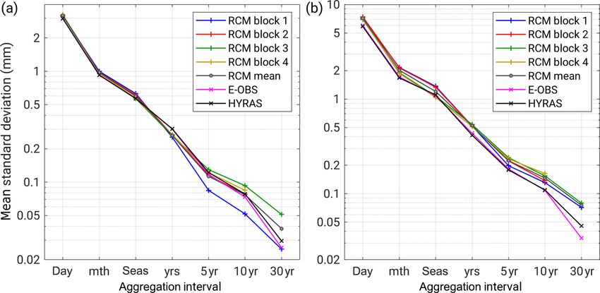
For ME, the evolution of the number of days exceeding
the climatological mean percentile reveals a strong positive
and significant trend for both the 99th (Fig. 8, top) and 99.9th
percentile (Fig. S10). The exact values of the climTP mean,
the linear regression, the relative change, and the significance
can be found in Table 4 (top numbers). For AL, the year-to-
year variability is higher and the overall trend is slightly neg- Figure 8. Deviation of the LAERTES-EU ensemble mean of
ative (Figs. 8, bottom, and S11) and at least significant for the the yearly number of days above the 99th percentile (wet days
only) of daily spatial mean precipitation compared to the clima-
99th percentile. Again, we analyze the trend for TP1b sepa-
tology (climTP; 1961–1990) for (a) Mid-Europe (ME) and (b) the
rately (Table 4, bottom numbers). The tendencies for TP1b Alps (AL). Red bars indicate negative anomalies (less days);
are the same but less pronounced except for the days exceed- blue bars indicate positive anomalies (more days). The predictions
ing the 99th percentile in AL, where there is a stronger trend (TP2; 2018–2028) are given in green. The black line indicates a lin-
signal in TP1b compared to the whole time series, which is ear regression.
also significant to a high degree.
5.2.2 Past trends and periodic oscillations in Fig. 9), some oscillations appear with phases of increasing
and decreasing precipitation. This signal might be smoothed,
For a more detailed analysis of trends, the Mann–Kendall as it is not expected that the decadal simulations of data
test described in Sect. 3.2 is applied to the time series of blocks 2 and 4 cover the natural variability at this timescale in
daily spatial mean precipitation percentiles. Figure 9a shows detail. Furthermore, these simulations are not expected to be
the relative number of LAERTES-EU members that show in phase with the long-lasting simulations of data blocks 1
a positive or negative trend of the 99th percentile for ME. and 3. The trends on this timescale reach rates of up to
Only cases in which more than 60 % of the complete ensem- 0.1 mm a−1 or 1 mm per decade, respectively. The overall
ble members reveal the same tendency are then considered trend is weaker with a rate of 0–0.02 mm a−1 or 0–2 mm per
for further investigation. For these cases, the ensemble mean century, respectively. Positive trends are more often signif-
trend is calculated (Fig. 9b) and the relative amount of signif- icant than the negative, while only a small part of the en-
icant members is displayed (Fig. 9c). All cases in which the semble shows significant trends. Similar results can be found
ensemble reveals ambiguous tendencies are neglected (gray for AL (Fig. S12). The trends on the decadal timescale reach
areas). higher rates but the oscillation is less pronounced than in ME.
To a high degree, the single members show the same be- Again, most of the positive trends are significant, while just
havior, especially for the longer time series where positive a few members with negative trends are significant.
trends are dominant. On a decadal timescale (diagonal line
https://doi.org/10.5194/esd-11-469-2020 Earth Syst. Dynam., 11, 469–490, 2020480 F. Ehmele et al.: Heavy precipitation in central Europe
Figure 9. Trend analysis of the 99th percentile (wet days only) of daily spatial mean precipitation for ME with (a) the relative amount of
members of LAERTES-EU with a positive (blue) or negative (red) trend; (b) the trend in millimeters per year averaged over the members
from panel (a), and (c) relative amount of members from panel (a) with a significant trend; cases with no distinct number (less than 60 %) of
members with same trend sign are marked in gray in panels (a)–(c).
For the 99.9th percentile of ME, large parts of LAERTES- Nevertheless, a more detailed trend analysis illustrated in
EU show positive trends (Fig. S13). On the decadal Fig. 9 and also Figs. S12–S14 reveals that LAERTES-EU
timescale, a clear sequence of positive and negative trends shows no clear tendency for the 99 % during TP2. Just in
is visible. Both the increases and decreases are more pro- a few cases, more than 60 % of the members have a simi-
nounced than for the 99th percentile but only a few members lar mainly positive trend signal, which, however, is not sig-
are significant. For AL, even more parts of the ensemble have nificant. In the case of the 99.9th percentile, 60 %–70 %
the same tendency of heavy precipitation and a higher num- of the members show a strong positive trend of more than
ber of members have a significant trend (Fig. S14). These 0.1 mm a−1 with 20 %–40 % of them being significant. Al-
trends exceed rates of decisively more than ±0.1 mm a−1 . In though the tendency for TP2 is ambiguous and less signifi-
contrast to the results above, the 99.9th percentile for AL cant, it shows continuity to the present decade.
seems to have a multidecadal oscillation, while the overall
trend of the complete time series is negative. 5.3 Climate change indices
The results described in the previous sections also manifest
5.2.3 Future predictions
in the considered ETCCDI climate change indices (Table 5).
With respect to the upcoming decade (TP2; 2018–2028), R95pTOT shows a positive trend for ME (Fig. 10a) with a
LAERTES-EU predicts a continuation of the current trend relative change of about 18 % and a strong negative trend of
with an increase especially for the 99.9th percentile (Figs. 7 approximately −15 % for AL (Fig. S15). Remarkably, there
and S6–S8; reddish area). In comparison to the last is a high positive deviation in the first half of the 20th cen-
decade (2007–2017), the RCM mean of the 99th percentile tury compared to the climTP amount for AL which might be
increases of about 0.6 % for ME and about 2.1 % for AL. The artificial due to the mentioned problems of the dry-day cor-
99.9th percentile increases about 2.0 % for ME and 3.0 % rection. R99pTOT shows a positive change for ME (Fig. 10b)
for AL. and a slightly negative trend for AL (Fig. S16). The overes-
Further to this absolute change, the number of days ex- timation for AL in the early century is less pronounced for
ceeding the climatological 99th percentile shows an increase this index. Considering only the TP1b, the tendencies are
of 4.9 % for ME and 8.4 % for AL, and 6.7 % (ME) and the same in all cases. The positive trends for ME are less
22.4 % (AL) in the case of the 99.9 % compared to the mean pronounced, while the negative trends for AL are stronger.
of 2007–2017. This also manifests in the relative anomaly The estimated trends are highly significant, except for the
(Figs. 8 and S10–S11; green bars). R99pTOT of AL for the whole time series.
Earth Syst. Dynam., 11, 469–490, 2020 https://doi.org/10.5194/esd-11-469-2020F. Ehmele et al.: Heavy precipitation in central Europe 481
Figure 10. Relative deviation of (a) the R95pTOT index and (b) the R99pTOT index of the LAERTES-EU ensemble mean of daily spatial
mean precipitation (wet days and land only) compared to the climatology (climTP; 1961–1990; Table 5) for Mid-Europe (ME). Red bars
indicate negative (dry) anomalies; blue bars indicate positive (wet) anomalies. The predictions (TP2; 2018–2028) are given in green. The
black line indicates a linear regression.
Table 5. Climatological mean (climTP; 1961–1990) of ETCCDI setup of the COSMO model remained the same for all simu-
quantities for Mid-Europe (ME) and the Alps (AL), linear regres- lations. In total, the presented LAERTES-EU consists of over
sion (LR) and relative change (RC) compared to climTP for differ- 1100 simulation runs with approximately 12 500 simulated
ent TPs, and related significance (p value; α = 0.05). Both indices years on a 25 km horizontal resolution.
are based on wet days only of daily spatial mean precipitation (land The focus of investigation was laid on the PRUDENCE re-
only).
gions Mid-Europe (ME) and the Alps (AL). Regarding inten-
sive areal precipitation, we concentrated on high percentiles,
Area ETCCDI climTP TP LR RC pα
namely 99 % and 99.9 %, of spatially averaged daily precipi-
(mm) (mm) (%)
tation amounts. Note that it was not expected that LAERTES-
ME R95pTOT 157.5 1+2 28.4 18 1.0 EU was able to reproduce historical precipitation events on a
1b 20.1 13 1.0 daily base in detail but have a more accurate performance re-
R99pTOT 43.8 1+2 15.6 36 1.0
garding long-term variations and statistical distributions on a
1b 12.2 28 1.0
larger scale perspective. Furthermore, the given resolution re-
AL R95pTOT 306.7 1+2 −46.3 −15 1.0 stricts the consideration of convective processes, so we con-
1b −54.3 −18 1.0 centrated on larger-scale phenomena.
R99pTOT 88.5 1+2 −4.5 −5 0.8953
With respect to our initial research questions, the follow-
1b −10.8 −12 0.9891
ing main conclusions can be drawn and summed up out of
the presented results, which will be discussed in more detail
afterwards:
Compared to the present decade, the predictions show a
continuation of the positive trend for ME with an increase of 1. LAERTES-EU is capable of representing the range of
2 % for R95pTOT and 5 % for R99pTOT. In contrast, both extreme areal precipitation similar to the used observa-
indices show a positive trend for AL with an increase of 7 % tional data sets and also fits into the range of previous
for R95pTOT and 8 % for R99pTOT, which is a complete studies (e.g., Früh et al., 2010). The four data blocks are
reversal of the overall trend. consistent and have similar precipitation distributions.
The ensemble also covers the observed temporal evolu-
tion.
6 Summary and conclusions
2. The benefits of the large ensemble size manifest in a
We have presented the novel LAERTES-EU ensemble com- strong increase of the signal-to-noise ratio beyond the
bining various regional climate model simulations done with typically used ensemble sizes and in high statistical sig-
COSMO-CLM to analyze long-term variability and trends of nificance of estimated trends for the ensemble mean.
flood-related intensive areal precipitation across central Eu- Furthermore, the distribution of precipitation totals is
rope. The whole RCM ensemble was divided into four data represented in a more concise way, taking the limita-
blocks depending on forcing data, assimilation schemes, or tions of the considered observations into account.
the initialization of the driving global model MPI-ESM. The
https://doi.org/10.5194/esd-11-469-2020 Earth Syst. Dynam., 11, 469–490, 2020You can also read