Analyses of temperature and precipitation in the Indian Jammu and Kashmir region for the 1980-2016 period: implications for remote influence and ...
←
→
Page content transcription
If your browser does not render page correctly, please read the page content below
Atmos. Chem. Phys., 19, 15–37, 2019
https://doi.org/10.5194/acp-19-15-2019
© Author(s) 2019. This work is distributed under
the Creative Commons Attribution 4.0 License.

Analyses of temperature and precipitation in the Indian Jammu and
Kashmir region for the 1980–2016 period: implications for remote
influence and extreme events
Sumira Nazir Zaz1 , Shakil Ahmad Romshoo1 , Ramkumar Thokuluwa Krishnamoorthy2 , and
Yesubabu Viswanadhapalli2
1 Department   of Earth Sciences, University of Kashmir, Hazratbal, Srinagar, Jammu and Kashmir 190006, India
2 National   Atmospheric Research Laboratory, Dept. of Space, Govt. of India, Gadanki, Andhra Pradesh 517112, India

Correspondence: Ramkumar Thokuluwa Krishnamoorthy (tkram@narl.gov.in)

Received: 23 February 2018 – Discussion started: 22 May 2018
Revised: 19 November 2018 – Accepted: 26 November 2018 – Published: 2 January 2019

Abstract. The local weather and climate of the Himalayas          decreases in spring precipitation. In the present study, the ob-
are sensitive and interlinked with global-scale changes in cli-   served long-term trends in temperature (◦ C year−1 ) and pre-
mate, as the hydrology of this region is mainly governed          cipitation (mm year−1 ) along with their respective standard
by snow and glaciers. There are clear and strong indica-          errors during 1980–2016 are as follows: (i) 0.05 (0.01) and
tors of climate change reported for the Himalayas, particu-       −16.7 (6.3) for Gulmarg, (ii) 0.04 (0.01) and −6.6 (2.9) for
larly the Jammu and Kashmir region situated in the west-          Srinagar, (iii) 0.04 (0.01) and −0.69 (4.79) for Kokarnag,
ern Himalayas. In this study, using observational data, de-       (iv) 0.04 (0.01) and −0.13 (3.95) for Pahalgam, (v) 0.034
tailed characteristics of long- and short-term as well as lo-     (0.01) and −5.5 (3.6) for Kupwara, and (vi) 0.01 (0.01)
calized variations in temperature and precipitation are an-       and −7.96 (4.5) for Qazigund. The present study also re-
alyzed for these six meteorological stations, namely, Gul-        veals that variation in temperature and precipitation during
marg, Pahalgam, Kokarnag, Qazigund, Kupwara and Srina-            winter (December–March) has a close association with the
gar during 1980–2016. All of these stations are located in        North Atlantic Oscillation (NAO). Further, the observed tem-
Jammu and Kashmir, India. In addition to analysis of sta-         perature data (monthly averaged data for 1980–2016) at all
tions observations, we also utilized the dynamical down-          the stations show a good correlation of 0.86 with the re-
scaled simulations of WRF model and ERA-Interim (ERA-I)           sults of WRF and therefore the model downscaled simula-
data for the study period. The annual and seasonal tempera-       tions are considered a valid scientific tool for the studies
ture and precipitation changes were analyzed by carrying out      of climate change in this region. Though the correlation be-
Mann–Kendall, linear regression, cumulative deviation and         tween WRF model and observed precipitation is significantly
Student’s t statistical tests. The results show an increase of    strong, the WRF model significantly underestimates the rain-
0.8 ◦ C in average annual temperature over 37 years (from         fall amount, which necessitates the need for the sensitivity
1980 to 2016) with higher increase in maximum tempera-            study of the model using the various microphysical param-
ture (0.97 ◦ C) compared to minimum temperature (0.76 ◦ C).       eterization schemes. The potential vorticities in the upper
Analyses of annual mean temperature at all the stations re-       troposphere are obtained from ERA-I over the Jammu and
veal that the high-altitude stations of Pahalgam (1.13 ◦ C)       Kashmir region and indicate that the extreme weather event
and Gulmarg (1.04 ◦ C) exhibit a steep increase and statis-       of September 2014 occurred due to breaking of intense at-
tically significant trends. The overall precipitation and tem-    mospheric Rossby wave activity over Kashmir. As the wave
perature patterns in the valley show significant decreases and    could transport a large amount of water vapor from both the
increases in the annual rainfall and temperature respectively.    Bay of Bengal and Arabian Sea and dump them over the
Seasonal analyses show significant increasing trends in the       Kashmir region through wave breaking, it probably resulted
winter and spring temperatures at all stations, with prominent    in the historical devastating flooding of the whole Kashmir

Published by Copernicus Publications on behalf of the European Geosciences Union.
16                         S. N. Zaz et al.: Analyses of temperature and precipitation in Jammu-Kashmir for 1980–2016

valley in the first week of September 2014. This was ac-          balanced-atmospheric-background condition, can be derived
companied by extreme rainfall events measuring more than          from PV and boundary conditions (Hoskins et al., 1985).
620 mm in some parts of the Pir Panjal range in the south            Divergence of the atmospheric air flows near the upper tro-
Kashmir.                                                          posphere is larger during precipitation, leading to increases
                                                                  in the strength of PV. Because of this, generally there will
                                                                  be a good positive correlation between variations in the
                                                                  strength of PV in the upper troposphere and precipitation
                                                                  over the ground, provided that the precipitation is mainly
1    Introduction                                                 due to the passage of large-scale atmospheric weather sys-
                                                                  tems like western disturbances and monsoons. Wind flows
Climate change is a phenomenon affecting the Earth’s atmo-        over topography can significantly affect the vertical distri-
sphere and surface which has in recent decades been shown         bution of water vapor and precipitation characteristics. Be-
to have significant effects on all spheres of life almost ev-     cause of this, positive correlation between variations in PV
erywhere in the world. Extreme weather events like anoma-         and precipitation can be modified significantly. These facts
lously large floods and unusual drought conditions associated     need to be taken into account while finding long-term varia-
with changes in climate play havoc with livelihoods of citi-      tions in precipitation near mountainous regions like the west-
zens even of developed societies, particularly in coastal and     ern Himalaya. The interplay between the flow of western dis-
mountainous areas. Jammu and Kashmir, India, located in           turbances and topography of the western Himalaya compli-
the western Himalayan region, is one such cataclysmically         cates further the identification of source mechanisms of ex-
formed mountainous region where the significant influence         treme weather events (Das et al., 2002; Shekhar et al., 2010)
of climate change on local weather has been observed for          like the ones that occurred in the western Himalayan region:
the last few decades: (1) shrinking and reducing glaciers,        Kashmir floods in 2014, Leh floods in 2010 in the Jammu
(2) devastating floods, (3) decreasing winter duration and        and Kashmir region, and Uttrakhand floods in 2013. Kumar
rainfall, and (4) increasing summer duration and temperature      et al. (2015) also noted that major flood events in the Hi-
(Solomon et al., 2007; Kohler and Maselli, 2009; Immerzeel        malayas are related to changing precipitation intensity in the
et al., 2010; Romshoo et al., 2015, 2017). Western distur-        region. This necessitates making use of proper surrogate pa-
bances (WDs) are considered one of the main sources of win-       rameters like PV and distinguishing between different source
ter precipitation for the Jammu and Kashmir region, which         mechanisms of extreme weather events associated with both
brings water vapor mainly from the tropical Atlantic Ocean,       the long-term climatic impacts of remote origin and short-
Mediterranean Sea, Caspian Sea and Black Sea. Though              term localized ones like organized convection (Romatschke
WD is perennial, it is most intense during northern winter        and Houze, 2011; Rasmussen and Houze, 2012; Rasmussen
(December–February). Planetary-scale atmospheric Rossby           and Houze Jr., 2016; Martius et al., 2012).
waves (RWs) have the potential to significantly alter the dis-       The main aim of the present study is to investigate long-
tribution and movement of WD according to their intensity         term (climate) variation in surface temperature and precip-
and duration (from a few to tens of days). Since WD is con-       itation over the Jammu and Kashmir region (western Hi-
trolled by planetary-scale Rossby waves in the whole tropo-       malayas) of India in terms of its connections with NAO and
sphere of the subtropical region, diagnosing different kinds      atmospheric Rossby wave activity in the upper troposphere.
of precipitation characteristics is easier with the help of po-   Since PV is considered a measure of Rossby wave activity,
tential vorticity (PV) at 350 K potential temperature (PT)        the present work analyses in detail, for a period of 37 years
and 200 hPa pressure surface (PS) as they are considered          during 1980–2016, monthly variation in PV (ERA-interim
proxies for Rossby wave activities (Ertel, 1942; Bartels et       reanalysis data, Dee et al., 2001) in the upper troposphere
al., 1998; Hunt et al., 2018a). Henceforth, it will be simply     (at 350 K and 200 hPa surfaces) and compares it with ob-
called PV at 350 K and 200 hPa surfaces. For example, Pos-        served surface temperature and rainfall (India Meteorolog-
tel and Hitchman (1999) and Hunt et al. (2018b) studied the       ical Department, IMD) at six widely separated mountainous
characteristics of Rossby wave breaking (RWB) events oc-          locations with variable orographic features (Srinagar, Gul-
curring at 350 K surfaces transecting the subtropical west-       marg, Pahalgam, Qazigund, Kokarnag and Kupwara). There
erly jets. Similarly, Waugh and Polvani (2000) studied RWB        exist several reports on climatological variation in meteoro-
characteristics at 350 K surfaces in the Pacific region during    logical parameters in various parts of the Himalayas. For ex-
northern fall–spring, with an emphasis on their influence on      ample, Kumar and Jain (2010) and Bhutiyani et al. (2010)
westerly ducts and their intrusion into the tropics. Since PV     found an increase in the temperature in the north-western
is a conserved quantity on isentropic and isobaric surfaces       Himalayas with significant variations in precipitation pat-
when there is no exchange of heat and pressure respectively,      terns. Archer and Fowler (2004) examined temperature data
it is widely used for investigating large-scale dynamical pro-    of seven stations in the Karakoram and Hindu Kush moun-
cesses associated with frictionless and adiabatic flows. More-    tains of the Upper Indus River Basin (UIRB) in search of
over, all other dynamical parameters, under a given suitable      seasonal and annual trends using statistical tests like regres-

Atmos. Chem. Phys., 19, 15–37, 2019                                                  www.atmos-chem-phys.net/19/15/2019/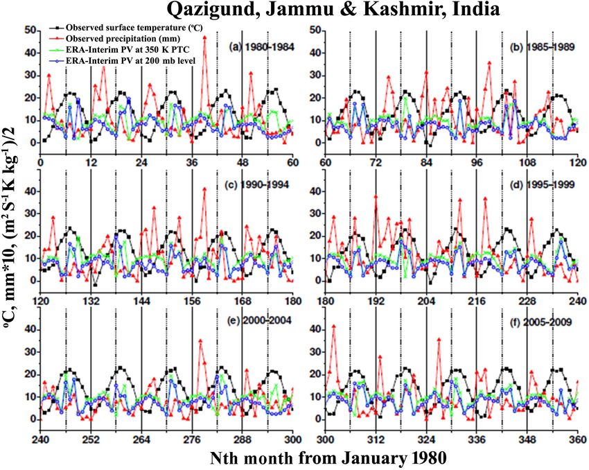
S. N. Zaz et al.: Analyses of temperature and precipitation in Jammu-Kashmir for 1980–2016                                           17

Figure 1. Geographical setting of the Kashmir valley (b) inside the Jammu and Kashmir state (a) of India (c) along with marked locations
of six meteorological observation stations: Srinagar, Gulmarg, Pahalgam, Kokarnag, Qazigund and Kupwara.

sion analysis. Their results revealed that mean winter max-           2   Geographical setting of Kashmir
imum temperature has increased significantly while mean
summer minimum temperature declined consistently. On the
                                                                      The mountainous valley of Kashmir has a unique geograph-
contrary, Liu et al. (2009) examined long-term trends in min-
                                                                      ical setting and it is located between the Greater Himalayas
imum and maximum temperatures over the Tibetan moun-
                                                                      in the north and Pir Panjal range in the south, roughly within
tain range during 1961–2003 and found that minimum tem-
                                                                      the latitude and longitude ranges of 33◦ 550 to 34◦ 500 N
perature increases faster than maximum temperature in all
                                                                      and 74◦ 300 to 75◦ 350 E respectively (Fig. 1). The heights
months. Romshoo et al. (2015) observed changes in snow
                                                                      of these mountains range from about 3000 to 5000 m and
precipitation and snowmelt runoff in the Kashmir valley and
                                                                      the mountains strongly influence the weather and climate
attributed the observed depletion of stream flow to the chang-
                                                                      of the region. Generally the topographic setting of the six
ing climate in the region. Bolch et al. (2012) reported that the
                                                                      stations, though variable, could be broadly categorized into
glacier extent in the Karakoram mountain range is increasing.
                                                                      two groups: (1) stations located on plains (Srinagar, Kokar-
   These contrasting findings of long-term variations in tem-
                                                                      nag, Qazigund and even Kupwara) and (2) those located in
perature and precipitation in the Himalayas need to be veri-
                                                                      the mountain setting (Gulmarg, Pahalgam). Physiographi-
fied by analyzing long-term climatological data available in
                                                                      cally, the valley of Kashmir is divided into three regions:
the region. However, the sparse and scanty availability of
                                                                      the Jhelum valley floor, Greater Himalayas and Pir Panjal.
regional climate data pose challenges in understanding the
                                                                      In order to represent all the regions of the valley, six meteo-
complex microclimate in this region. Therefore, studying the
                                                                      rological stations located widely with different mean sea lev-
relationship of recorded regional (Jammu and Kashmir) cli-
                                                                      els (m.s.l.), namely, Gulmarg (2740 m), Pahalgam (2600 m),
matic variations in temperature and precipitation with remote
                                                                      Kokarnag (2000 m), Srinagar (1600 m), Kupwara (1670 m)
and large-scale weather phenomena such as the NAO and
                                                                      and Qazigund (1650 m), were selected for analyses of ob-
El Niño Southern Oscillation (ENSO) is necessary for un-
                                                                      served weather parameters.
derstanding the physical processes that control the locally
                                                                         The Kashmir valley is one of the important watersheds
observed variations (Ghasemi, 2015). Archer and Fowler
                                                                      of the upper Indus basin, harboring more than 105 glaciers,
(2004) and Iqbal and Kashif (2013) found that large-scale
                                                                      and it experiences the mediterranean type of climate with
atmospheric circulation like NAO significantly influences
                                                                      marked seasonality (Romshoo and Rashid, 2014). Broadly,
the climate of the Himalayas. However, detailed informa-
                                                                      four seasons (Khattak et al., 2011; Rashid et al., 2015) are
tion about the variation in temperature and precipitation and
                                                                      defined for the Kashmir valley: winter (December to Febru-
its teleconnection with observed variations in NAO is inade-
                                                                      ary), spring (March to May), summer (June to August) and
quately available for this part of the Himalayan region (Kash-
                                                                      autumn (September to November). It is to be clarified here
mir Valley).
                                                                      that while defining the period of NAO (Fig. 4) considered

www.atmos-chem-phys.net/19/15/2019/                                                          Atmos. Chem. Phys., 19, 15–37, 2019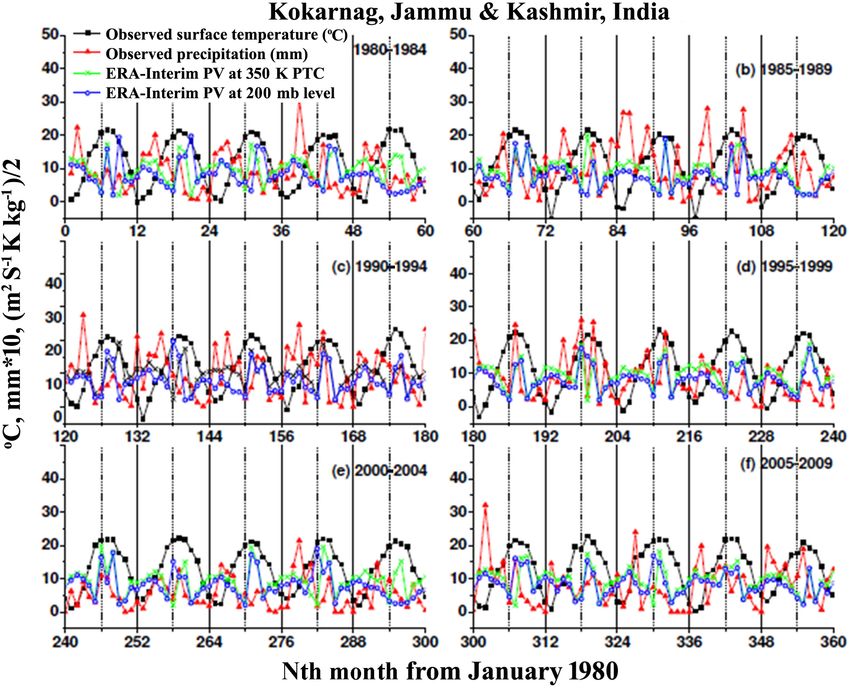
18                         S. N. Zaz et al.: Analyses of temperature and precipitation in Jammu-Kashmir for 1980–2016

December–March to be winter months as defined by Archer           in time series of temperature and precipitation was identified
and Fowler (2004) and Iqbal and Kashif (2013) and in all          using cumulative deviation test and Student’s t test (Pettitt,
other parts of the paper it is December–February as per the       1979). This method detects the time of significant change in
IMD definition. The annual temperature in the valley varies       the mean of a time series when the exact time of the change
from about −10 to 35 ◦ C. The rainfall pattern in the valley is   is unknown (Gao et al., 2011).
dominated by wintertime precipitation associated with west-          Winter NAO index during 1980–2010 were obtained for
ern disturbances (Dar et al., 2014) while the snow precipita-     further analyses from Climatic Research Unit through the
tion is received mainly in winter and early spring (Kaul and      web link https://www.cru.uea.ac.uk/data, last access: 17 De-
Qadri, 1979).                                                     cember 2018. The winter (December–March) NAO index is
                                                                  based on difference of normalized sea level pressure (SLP)
                                                                  between Lisbon, Portugal and Iceland, which is available
3     Data and methodology                                        from 1964 onwards. Positive NAO index is associated with
                                                                  stronger-than-average westerlies over the middle latitudes
The India Meteorological Department provided 37 years             (Hurrell and van Loon, 1997). The correlation between mean
(1980–2016) of data of daily precipitation, maximum and           (December–March) temperature, precipitation and NAO in-
minimum temperatures for all six stations. Monthly aver-          dex was determined using the Pearson correlation coefficient
aged data were further analyzed to find long-term variations      method. To test whether the observed trends in winter tem-
in weather parameters. Statistical tests including Mann–          perature and precipitation are enforced by NAO, linear re-
Kendall, Spearman’s rho, cumulative deviation and Student’s       gression analysis (forecast) was performed (Fig. 4e and f).
t test were performed to determine long-term trends and           The following algorithm calculates or predicts a future value
turning points of weather parameters with statistical signifi-    by using existing values. The predicted value is a y value
cance. Similar analyses and tests were also performed for the     for a given w value. The known values are existing w values
Weather and Research Forecasting (WRF) model-simulated            and y values, and the new value is predicted by using linear
and ERA-Interim reanalysis data (0.75◦ by 0.75◦ spatial res-      regression.
olution in the horizontal plane, monthly averaged time reso-         The syntax is as follows:
lution) of same weather parameters and for the NAO index.
A brief description of these data sets is provided below.         FORECAST(x, known_y’s, known_w’s).

3.1    Measurements and model simulations                         W is the data point for which we want to predict a value.
                                                                  Known_y’s is the dependent array or range of data (rainfall
The obtained observational data are analyzed carefully for        or temperature), and Known_w’s is the independent array or
homogeneity and missing values. Analyses of ratios of tem-        range of data (time).
perature from the neighboring stations with the Srinagar sta-        The equation for FORECAST is a + bw, where
tion were conducted using a relative homogeneity test (World                            X                   X
                                                                  a = ŷ − bŵ and b =    (w − ŵ)(y − ŷ)/  (w − ŵ)2 (1)
Meteorological Organization, 1970). It is found that there
is no significant inhomogeneity and data gap for any sta-         and where ŵ and ŷ are the sample means AVERAGE
tion. Few missing data points were linearly interpolated and      (known_w’s) and AVERAGE (known y’s).
enough care was taken not to make any meaningful inter-
pretation during such short periods of data gaps in the ob-       3.2   WRF model configuration
servations. Annual and seasonal means of temperature and
precipitation were calculated for all the stations and years.     The Advanced Research WRF version 3.9.1 model simula-
To compute seasonal means, the data were divided into the         tion was used in this study to downscale the ERA-Interim
following seasons: winter (December to February), spring          (European Centre for Medium-Range Weather Forecasts re-
(March to May), summer (June to August) and autumn                analysis) data over the Indian monsoon region. The model
(September to November). Trends in the annual and sea-            is configured with 2 two-way nested domains (18 and 9 km
sonal means of temperature and precipitation were deter-          horizontal resolutions), 51 vertical levels and model top at
mined using Mann–Kendall (nonparametric test) and linear          10 hPa level. The model first domain extends from 24.8516◦
regression tests (parametric test) at the confidence levels of    to 115.148◦ longitude and from −22.1127 to 46.7629◦ lat-
S = 99 % or (0.01), S = 95 % or 0.05 and S = 90 % or 0.1.         itude while the second domain covers from 56.3838◦ to
These tests have been extensively used in hydrometeorolog-        98.5722◦ longitude and from −3.86047 to 38.2874◦ latitude.
ical data analyses as they are less sensitive to heterogeneity       The initial and boundary conditions supplied to the WRF
of data distribution and least affected by extreme values or      model are obtained from ERA-Interim 6-hourly data. The
outliers in data series. Various methods have been applied to     model physics used in the study for boundary layer processes
determine change points of a time series (Radziejewski et al.,    is Yonsei University’s nonlocal diffusion scheme (Hong et
2000; Chen and Gupta, 2012). In this study, a change point        al., 2006), the Kain–Fritsch scheme for cumulus convec-

Atmos. Chem. Phys., 19, 15–37, 2019                                                  www.atmos-chem-phys.net/19/15/2019/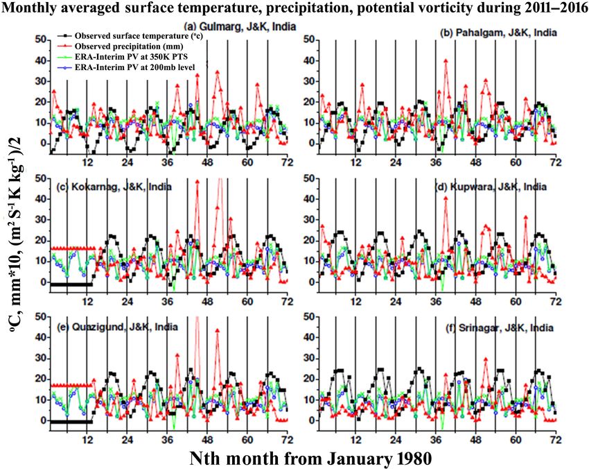
S. N. Zaz et al.: Analyses of temperature and precipitation in Jammu-Kashmir for 1980–2016                                                 19

Figure 2. Trends in surface temperature (◦ C) at the six interested locations of the Kashmir valley (a) for annual mean temperature, (b) maxi-
mum temperature, (c) minimum temperature, (d) winter mean temperature during December–February, (e) spring mean temperature (March–
May), (f) summer mean temperature (June–August) and (g) autumn mean temperature (September–November).

tion (Kain and Fritsch, 1993), Thomson scheme for micro-                 ulated temperature against the observed temperature data of
physical processes, the Noah land surface scheme (Chen and               IMD.
Dudhia, 2001) for surface processes, Rapid Radiation Trans-
fer Model (RRTM) for long-wave radiation (Mlawer et al.,
1997), and the Dudhia (1989) scheme for short-wave radia-                4     Results and discussion
tion. The physics options configured in this study are adopted
based on the previous studies of heavy rainfall and monsoon              4.1    Trend in annual and seasonal temperature
studies over the Indian region (Srinivas et al., 2013, 2018;
Madala et al., 2014; Priyanka et al., 2016).                             Tables 1 and 2 show the results of statistical tests (Mann–
   For the present study, the WRF model is initialized on a              Kendall and linear regression, cumulative deviation and Stu-
daily basis at 12:00 UTC using ERA-Interim data and inte-                dent’s t) carried out on the temperature and precipitation
grated for a 36 h period using the continuous re-initialization          data respectively. All the parametric and nonparametric tests
method (Lo et al., 2008; Langodan et al., 2016; Viswanad-                carried out for the trend analysis and abrupt changes in
hapalli et al., 2017). Keeping the first 12 h as model spin-up           the trend showed almost similar results. Table 1 therefore
time, the remaining 24 h daily simulations of the model are              shows results of representative tests where higher values
merged to get the data during 1980–2016. To find out the skill           of statistical significance between Mann–Kendall–linear re-
of the model, the downscaled simulations of the WRF model                gression test and cumulative deviation–Student’s t test are
are validated for six IMD surface meteorological stations.               considered. It is evident that there is an increasing trend
The statistical skill scores such as bias, mean error (ME) and           at different confidence levels in annual and seasonal tem-
root mean square error (RMSE) were computed for the sim-                 peratures of all six stations (Pahalgam, Gulmarg, Kokar-

www.atmos-chem-phys.net/19/15/2019/                                                              Atmos. Chem. Phys., 19, 15–37, 2019
20                                     S. N. Zaz et al.: Analyses of temperature and precipitation in Jammu-Kashmir for 1980–2016

Table 1. Annual and seasonal temperature trends in the Kashmir Valley during 1980–2016.

   Stationsa                   Temperature trends         Annual          Min        Max        Winter      Spring     Summer     Autumn       Abrupt change
   (Mann–Kendall test)                                                                                                                       (Student’s t test)
   Gulmarg                     Increasing trend           S = 0.01        S = 0.01   S = 0.1    S = 0.05    S = 0.01   NS         S = 0.05                1995
                               Z statistics               3.976           3.059      1.564      2.43        2.806      0.486      2.159
   Pahalgam                    Increasing trend           S = 0.01        S = 0.01   S = 0.01   S = 0.01    S = 0.01   S = 0.1    S = 0.05                1995
                               Z statistics               4.119           3.6        3.519      3.118       3.438      1.71       2.416
   Srinagar                    Increasing trend           S = 0.05        S = 0.1    S = 0.01   S = 0.05    S = 0.05   S = 0.1    NS                      1995
                               Z statistics               2.108           1.392      2.804      1.992       2.413      0.374      0.198
   Kupwara                     Increasing trend           S = 0.01        S = 0.1    S = 0.01   S = 0.05    S = 0.01   S = 0.1    S = 0.1                 1995
                               Z statistics               3.433           1.819      3.246      1.988       2.719      1.78       1.865
   Kokarnag                    Increasing trend           S = 0.01        S = 0.05   S = 0.01   S = 0.01    S = 0.01   S = 0.1    S = 0.1                 1995
                               Z statistics               3.467           2.363      3.11       3.195       3.195      1.46       0.68
   Qazigund                    Increasing trend           S = 0.1         S = 0.1    S = 0.1    S = 0.05    S = 0.05   NS         S = 0.1                 1995
                               Z statistics               1.717           1.77       1.68       2.026       2.236      −0.714     −1.501

a Critical values: a = 0.10 (1.654); a = 0.05 (1.96); a = 0.01 (2.567).

Table 2. Annual and seasonal precipitation trends in Kashmir valley during 1980–2016.

           Stationsa                       Precipitation trends           Annual      Winter     Spring       Summer      Autumn       Abrupt change
           (Mann–Kendall test)                                                                                                       (Student’s t test)
           Gulmarg                         Decreasing trend               S = 0.05    S = 0.1    S = 0.01     NS          NS                      1995
                                           Z statistics                   −1.988      −1.53      −2.515       −0.445      −0.394
           Pahalgam                        Decreasing trend               S = 0.1     S = 0.1    S = 0.05     NS          NS                      1995
                                           Z statistics                   −1.442      −1.136     −2.151       −0.556      0.034
           Srinagar                        Decreasing trend               S = 0.05    NS         S = 0.01     NS          NS                      1995
                                           Z statistics                   −2.532      0.051      −2.060       −0.105      −1.003
           Kupwara                         Decreasing trend               S = 0.1     S = 0.1    S = 0.01     NS          NS                      1995
                                           Z statistics                   −1.962      −0.817     −2.919       −0.986      −0.153
           Kokarnag                        Decreasing trend               S = 0.1     S = 0.1    S = 0.05     NS          NS                      1995
                                           Z statistics                   −1.326      −1.53      −2.276       0.186       −0.119
           Qazigund                        Decreasing trend               S = 0.05    NS         S = 0.05     NS          NS                      1995
                                           Z statistics                   −1.275      −0.764     −2.413       0.359       −0.232
         a Critical values: a = 0.10 (1.654); a = 0.05 (1.96); a = 0.01 (2.567).

nag, Srinagar, Kupwara and Qazigund), located in differ-                                      Analyses of maximum and minimum temperatures (Ta-
ent topographical settings (Table 3). During 1980–2016, Pa-                                ble 1 and Fig. 2b) for the six stations reveal a higher rate of
halgam and Gulmarg, located at higher elevations of about                                  increase in maximum temperature. Pahalgam and Kupwara
2500 m a.m.s.l. (above mean sea level), registered statisti-                               recorded the highest rise of ∼ 1.3 ◦ C, followed by Kokarnag
cally significant increases in average annual temperature by                               (1.2 ◦ C) and Srinagar (1.1 ◦ C). The exception is that Gul-
1.13 and 1.04 ◦ C (Fig. 2a). It should be noted that hereafter                             marg and Qazigund (being a hilly station) shows less than
the period 1980–2016 will not be mentioned explicitly, and                                 0.6 ◦ C in maximum temperature. The minimum temperature
statistically significant means the confidence level is about                              exhibits the lowest increase of 0.3 ◦ C at Srinagar and high-
90 %. Kokarnag and Kupwara, located at the heights of about                                est increase at Gulmarg station of 1.2 ◦ C (Fig. 2c). Analy-
1800–2000 m a.m.s.l., showed increases of 0.9 and 1 ◦ C re-                                ses of composite seasonal mean of minimum and maximum
spectively (Fig. 2a). However, Srinagar and Qazigund, lo-                                  temperatures in the valley reveal a higher increase in maxi-
cated at the heights of about 1700–1600 m a.m.s.l., exhibited                              mum temperature in winter and spring seasons. Among four
increases of 0.65 and 0.44 ◦ C (Fig. 2a).                                                  stations (Gulmarg, Pahalgam, Kokarnag and Kupwara), Gul-
                                                                                           marg indicates an increase of less than 1 ◦ C while Pahalgam,

Atmos. Chem. Phys., 19, 15–37, 2019                                                                              www.atmos-chem-phys.net/19/15/2019/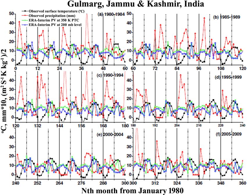
S. N. Zaz et al.: Analyses of temperature and precipitation in Jammu-Kashmir for 1980–2016                                          21

Table 3. Mean temperature increases at each station during 1980–2016.

         Stations     Elevation in meters   Topography                                                      Increase in annual
                                                                                                            temperature in ◦ C
         Pahalgam                   2600    Located on mountain top                                                      1.13
         Gulmarg                    2740    Located on mountain top                                                      1.04
         Srinagar                   1600    Located on plane surface in an urbanized area                                0.55
         Kupwara                    1670    Located on plane surface bounded on three sides by mountains                 0.92
         Kokarnag                   2000    Located on plane surface                                                     0.99
         Qazigund                   1650    Located on plane surface                                                     0.78

Kokarnag and Kupwara show increases of 0.9, 0.9 and less                cipitation. Results reveal that the year 1995 is the year of
than 0.9 ◦ C respectively (Table 1 and Fig. 2d). On the con-            abrupt increase (change point) in the temperature of the val-
trary, Qazigund and Srinagar showed a slight increase of less           ley (Fig. 4a) and the same year is identified as the year of
than 0.4 and 0.5 ◦ C respectively. The mean spring tempera-             abrupt decrease for precipitation (Fig. 4b).
ture shows a higher rise compared to other seasons tempera-
tures for all stations. Gulmarg shows an increase of less than          4.3   Influence of North Atlantic Oscillation (NAO) on
1.4 ◦ C. Pahalgam, Kupwara and Kokarnag showed increases                      the winter precipitation over the Kashmir valley
of 1.3 ◦ C at S = 0.01. Qazigund and Srinagar revealed 0.6
and 1 ◦ C increase respectively as shown in the Table 1 and             The present study also investigates the teleconnection be-
Fig. 2e. In summer, the temperature rise for Pahalgam is                tween the activity of the NAO and the variations in tem-
about less than 0.6 ◦ C and for Gulmarg and Qazigund, it is             perature and precipitation over the Kashmir valley, partic-
about 0.4 and 0.2 ◦ C respectively (Table 1). Kupwara, Kokar-           ularly during the winter season (December–March). It is
nag and Srinagar reveal an increase of less than 0.3, 0.4 and           found that there is a significant negative/positive correla-
0.1 ◦ C respectively (Fig. 2f). In autumn, Gulmarg shows an             tion (−0.54/0.68) between NAO (NAO index) and precipita-
increase of 0.9 ◦ C and Pahalgam exhibits less than 0.6 ◦ C. On         tion/temperature (Fig. 4c). This suggests that winter precip-
the contrary Qazigund shows less than 0.4 ◦ C increase while            itation and temperature over the Kashmir valley has a close
Srinagar shows no significant increase in observed tempera-             association with the winter NAO. Higher precipitation over
tures (Fig. 2g and Table 1).                                            Kashmir is associated with a positive phase of NAO. Fur-
                                                                        ther the “change point” year, 1995, in the trend of tempera-
4.2   Trend in annual and seasonal precipitation                        ture and precipitation coincides with that of the NAO index.
                                                                        To test whether the trends in temperatures and precipitation
The annual precipitation pattern of the valley is comparable            over the Kashmir valley are forced by the NAO, regression
to that of temperature, with a higher decrease observed at the          analysis was performed on winter temperature and precipi-
upper elevation stations of Gulmarg and Pahalgam (Fig. 3a               tation (Fig. 4e and f) and the results indicate that there is a
and Table 2). Similar to temperature, Table 2 provides in de-           significant connection between NAO and precipitation over
tail the test results of Mann–Kendall, linear regression and            Kashmir.
Student’s t. While Kokarnag and Kupwara show significant                   The observed annual and seasonal variation in temperature
decrease, the lower elevated stations, Qazigund and Srina-              at all stations except Qazigund is strongly correlated with
gar, exhibit insignificant decreases (Fig. 3a). The decrease in         WRF downscaled simulations. Overall, the simulations show
winter precipitation is maximum at Gulmarg and Kokarnag                 correlation of 0.66, 0.67, 0.72, 0.62, 0.79 and 0.47 for Sri-
followed by Kupwara and Pahalgam and it is an insignificant             nagar, Gulmarg, Kokarnag, Kupwara, Pahalgam and Qazi-
decrease for Srinagar and Qazigund (Table 2 and Fig. 3b).               gund respectively. The annual mean simulated temperature
The spring season precipitation exhibits a decreasing trend             shows very good correlation (0.85) with observations. Fig-
for all six stations, with the lowest decrease of 42 mm pre-            ure 5 shows annual and seasonal correlations between trends
cipitation at Kupwara (Table 2).                                        of observed and simulated temperatures (location of Kokar-
   During summer months, precipitation also shows a de-                 nag is considered for WRF data). However, RMSE analy-
creasing trend for all stations except Qazigund that it is sta-         sis indicates that model simulations slightly underestimate
tistically insignificant (Fig. 3d, and Table 2). For Qazigund           the observations by an average value of 0.43 ◦ C. Similar to
there is no apparent trend in summer precipitation. The au-             Fig. 5, Fig. 6 shows the comparison between WRF model
tumn precipitation also shows an insignificant decreasing               simulated and observed precipitation. Even though the trend
trend for the stations (Fig. 3e and Table 2). Cumulative test-          is similar, the WRF model severely underestimates the rain-
ing was used to determine the “change point” of the trend               fall amount. A detailed study on this topic will be presented
in the annual and seasonal variations in temperature and pre-           in a separate paper.

www.atmos-chem-phys.net/19/15/2019/                                                           Atmos. Chem. Phys., 19, 15–37, 2019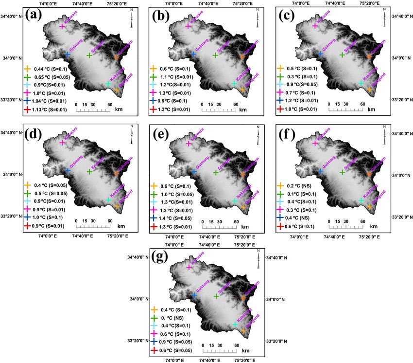
22                           S. N. Zaz et al.: Analyses of temperature and precipitation in Jammu-Kashmir for 1980–2016

Figure 3. Same as Fig. 2 but for precipitation (mm) and only for means of (a) annual, (b) winter, (c) spring, (d) summer and (e) autumn.

Figure 4. (a) Cumulative testing for defining change point of temperature (averaged for all six stations of the Kashmir valley), (b) same as
(a) but for precipitation, (c) comparison of trends of Kashmir temperature with North Atlantic Ocean (NAO) index, (d) same as (c) but for
precipitation, (e) regression analysis of winter temperature and (f) regression analysis of winter precipitation.

Atmos. Chem. Phys., 19, 15–37, 2019                                                           www.atmos-chem-phys.net/19/15/2019/
S. N. Zaz et al.: Analyses of temperature and precipitation in Jammu-Kashmir for 1980–2016                                             23

Figure 5. (a) Comparision between observed and WRF model (location of Kokarnag is considered) simulated annually averaged temperature
(averaged for all the stations) variations for the years 1980–2016, (b) same as (a) but for spring season, (c) for summer, (d) for autumn,
(e) winter, (f) for minimum temperature and (g) maximum temperature.

4.4   Discussion                                                       study, it is observed that rises in temperature are larger at the
                                                                       higher-altitude stations of Pahalgam (1.13 ◦ C) and Gulmarg
The Himalayan mountain system is quite sensitive to global             (1.04 ◦ C) and they are about 0.9, 0.99, 0.04 and 0.10 ◦ C for
climate change as the hydrology of the region is mainly dom-           the other stations, Kokarnag, Kupwara, Srinagar and Qazi-
inated by snow and glaciers, making it one of the ideal sites          gund respectively during 1980–2016. Liu et al. (2009) and
for early detection of global warming (Solomon et al., 2007;           Liu and Chen (2000) also report higher warming trends at
Kohler and Maselli, 2009). Various reports claim that in the           higher altitudes in the Himalayan regions. In the future, the
Himalayas significant warming occurred in the last century             impacts of climate change will be intense at higher elevations
(Fowler and Archer, 2006; Bhutiyani et al., 2007). Shrestha            and in regions with complex topography, which is consistent
et al. (1999) analyzed surface temperature at 49 stations lo-          with the model results of Wiltshire (2013).
cated across the Nepalese Himalayas and the results indi-                 A noteworthy observation in the present study is that
cate warming trends in the range of 0.06 to 0.12 ◦ C per year.         statistically significant steep increase in the temperature
The observations of the present study are in agreement with            (change point) occurred in the year 1995 and it has been
the studies carried out by Shrestha et al. (1999), Archer and          continuing thereafter. The mega El Niño in 1998 is consid-
Fowler (2004) and Bhutiyani et al. (2007). In the present

www.atmos-chem-phys.net/19/15/2019/                                                            Atmos. Chem. Phys., 19, 15–37, 2019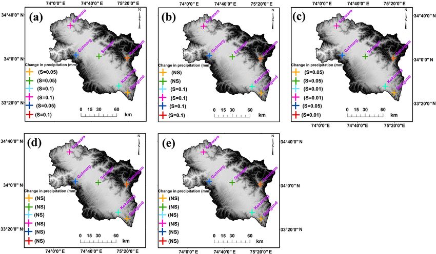
24                          S. N. Zaz et al.: Analyses of temperature and precipitation in Jammu-Kashmir for 1980–2016

Figure 6. Same as Fig. 5 but for precipitation. Here the minimum and maximum precipitation values are not considered because they cannot
be defined properly within a day.

ered one of the strongest El Niño events in history and led           duction in the percentage of snow and glacier can alter the
to a worldwide increase in temperature. Contrastingly, the            surface albedo over a region, which in turn can increase the
El Niño in 1992 led to a decrease in temperature through-             surface air temperatures (Kulkarni et al., 2002; Groisman et
out the Northern Hemisphere, which is ascribed to the                 al., 1994). Romshoo et al. (2015) and Murtaza and Romshoo
Mt Pinatabu volcanic eruption (Swanson et al., 2009; IPCC,            (2016) have also reported that a reduction in snow and glacier
2013). Also, this event prevented direct sunlight reaching            cover in the Kashmir regions of the Himalayas during recent
some areas of the surface of the Earth for about 2 months             decades could be one of the reasons for the occurrence of
(Barnes et al., 2016).                                                higher warming, particularly on the higher elevated stations
   Studies of trends in seasonal-mean temperature in many             of Gulmarg and Pahalgam.
regions across the Himalayas indicate higher warming trends              In the Himalayan mountain system, contrasting trends
in winter and spring months (Shrestha et al., 1999; Archer            have been noted in precipitation over recent decades (IPCC,
and Fowler, 2004; Bhutiyani et al., 2009). The seasonal dif-          2001). Borgaonkar and Pant (2001), Shrestha (2000) and
ference found in the present study is consistent with other           Archer and Fowler (2004) observed increasing precipitation
studies carried out for the Himalayas (Archer and Fowler,             patterns over the Himalayas while Mooley and Parthasarthy
2004; Sheikh et al., 2009; Roe et al., 2003); Lancang Val-            (1984), Kumar and Jain (2010) and Dimri and Dash (2012)
ley, China (Yunling and Yiping, 2005); Tibet (Liu and Chen,           reported large-scale decadal variation with increasing and
2000) and the Swiss Alps (Beniston, 2010), where almost all           decreasing precipitation periods. The results of the present
stations recorded a higher increase in the winter and spring          study indicate that the decrease in annual precipitation is
temperatures compared to autumn and summer temperatures.              slightly insignificant at all six stations except in the spring
Recent studies found that a reduction in the depth of snow            season. The increasing trend in temperature can trigger large-
cover and shrinking glaciers may also be one of the con-              scale energy exchanges that become more intricate as com-
tributing factors for the observed higher warming, as the re-         plex topography alters the precipitation type and intensity in

Atmos. Chem. Phys., 19, 15–37, 2019                                                        www.atmos-chem-phys.net/19/15/2019/
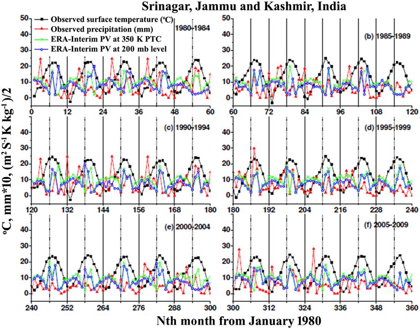
S. N. Zaz et al.: Analyses of temperature and precipitation in Jammu-Kashmir for 1980–2016                                                25

Figure 7. Observed monthly averaged surface temperature and precipitation as well as ERA-interim potential vorticities at the 350 K potential
temperature and 200 hPa pressure surfaces for the Srinagar station during the years 1980–2016.

many ways (Kulkarni et al., 2002; Groisman et al., 1994).                found a strong connection between the NAO and temperature
Climate model simulations (Zarenistana et al., 2014; Rashid              and precipitation in the north-western Himalayas (Archer
et al., 2015) and empirical evidence (Vose et al., 2005;                 and Fowler, 2004; Bhutiyani et al., 2007; Bookhagen, 2010;
Romshoo et al., 2015) also confirm that increasing tempera-              Sharif et al., 2013; Iqbal and Kashif, 2013). A substantial
ture results in increased water vapor, leading to more intense           fraction of the most recent warming is linked to the behavior
precipitation events even when the total annual precipitation            of the NAO (Hurrell and van Loon, 1997; Thompson et al.,
reduces slightly. The increase in temperature therefore en-              2003; Madhura et al., 2015). The climate of the Kashmir Hi-
hances the risks of both floods and droughts. For example,               malayas is influenced by western disturbances in winter and
the disaster flood event of September 2014 occurred in the               spring seasons. Figure 4c and d show correlation between
Kashmir valley due to high-frequency and high intense pre-               wintertime NAO and temperature and precipitation over the
cipitation.                                                              Kashmir region. While temperature shows a negative corre-
   The NAO is one of the strongest northern atmospheric                  lation of −0.54, precipitation shows a positive correlation of
weather phenomena occurring due to the difference of at-                 0.68. From linear regression analyses, it is found that consid-
mospheric pressure at sea level between the Iceland low and              erable variation in winter precipitation and temperature over
Azores high. It controls the strength and direction of west-             Kashmir is forced by winter NAO. The weakening link of
erly winds across the Northern Hemisphere. Surface tem-                  NAO after 1995 has a close association with decreased winter
peratures have increased in the Northern Hemisphere in the               precipitation and increased winter temperature in the valley.
past few decades (Mann et al., 1999; Jones et al., 2001; Hi-             Similarly, Bhutiyani et al. (2009) and Dimri and Dash (2012)
jioka et al., 2014), and the rate of warming has been espe-              also found a statistically significant decreasing trend in pre-
cially high (∼ 0.15 ◦ C decade−1 ) in the past 40 years (Fol-            cipitation which they related to weakening of NAO index.
land et al., 2001; Hansen et al., 2001; Peters et al., 2013;             However, to establish a detailed mechanism, incorporating
Knutti et al., 2016). The NAO causes substantial fluctuations            these variations requires thorough investigation.
in the climate of the Himalayas (Hurrell and van Loon, 1997;                The WRF model simulations compare well with observa-
Syed et al., 2006; Archer and Fowler, 2004). Several workers             tions (significantly strong correlation of 0.85) and the corre-

www.atmos-chem-phys.net/19/15/2019/                                                              Atmos. Chem. Phys., 19, 15–37, 2019
26                          S. N. Zaz et al.: Analyses of temperature and precipitation in Jammu-Kashmir for 1980–2016

Figure 8. Same as Fig. 6 but for Kokarnag.

lation is more for the elevated stations than the valley stations   herent over many days and propagate long distances of the
of Srinagar and Kupwara. However, it is expected that a good        order of synoptic to planetary scales, leading to the telecon-
correlation can result if more precise terrain information is       nection of remote atmospheres of global extent. The study by
incorporated in the WRF model simulations. Earlier studies          Chang and Yu (1999) indicates that during northern winter
(e.g. Kain and Fritsch, 1990, 1993; Kain, 2004) also found          months of December–January–February, Rossby wave pack-
good correlation between observed and WRF simulated rain-           ets can be most coherent over a large distance of from the
fall events. In conjunction with large-scale features such as       northern Africa to the Pacific through southern Asia. There
NAO and ENSO, it can result in large-scale variability in the       are reports of extreme weather events connected to Rossby
climate of this region (Ogura and Yoshizaki, 1988). Further-        waves of synoptic to planetary scales in the upper tropo-
more, incorporation of mesoscale teleconnections and their          sphere (e.g. Screen and Simmonds, 2014). In northern India,
associations in the WRF model can further help in under-            there is an increasing trend in heavy rainfall events, partic-
standing large-scale weather forecasting over this region.          ularly over the Himachal Pradesh, Uttrakhand, and Jammu
                                                                    and Kashmir (Sinha Ray and Srivastava, 2000; Nibanupudi
4.5   Physical mechanisms of climate and weather of                 et al., 2015). Long Rossby waves can lead to the generation
      Jammu and Kashmir                                             of alternating convergence and divergence in the upper tro-
                                                                    posphere that in turn can affect surface weather parameters
Large-scale spatial and temporal variations in the meridional       like precipitation through the generation of instabilities in the
winds could be due to the passage of planetary-scale Rossby         atmospheric air associated with convergence and divergence
waves in the atmospheric winds. When RWs break in the up-           (Niranjan Kumar et al., 2016).
per troposphere, it could lead to vertical transport of atmo-          Using observations and MERRA (Modern-Era Retrospec-
spheric air between the upper troposphere and lower strato-         tive Analysis for Research and Applications reanalysis; https:
sphere and an irreversible horizontal transport of air mass be-     //gmao.gsfc.nasa.gov/research/merra/, last access: 19 De-
tween the subtropics and extratropics (McIntyre and Palmer,         cember 2018) data, Rienecker et al. (2011) showed strong
1983). Rossby waves have the characteristic of remaining co-        correlation between 6–10 days periodic oscillations associ-

Atmos. Chem. Phys., 19, 15–37, 2019                                                     www.atmos-chem-phys.net/19/15/2019/
S. N. Zaz et al.: Analyses of temperature and precipitation in Jammu-Kashmir for 1980–2016 27 Figure 9. Same as Fig. 7 but for Kupwara. ated with Rossby waves in the upper tropospheric winds strong association between enhanced Rossby wave activ- and surface weather parameters like atmospheric pressure, ity, surface temperature and extreme precipitation events in winds, temperature, relative humidity and rainfall during a 1979–2012. Since slowly propagating Rossby waves can in- severe weather event observed at the Indian extratropical sta- fluence weather at a particular site for long periods lasting tion, Nainital (29.45◦ , 79.5◦ ), in November–December 2011. more than few weeks, it is can be seen the imprint of climatic They also note that when the upper troposphere shows di- variations in Rossby waves in weather events from monthly vergence, the lower troposphere shows convergence and as mean atmospheric parameters. a result more moisture gets accumulated there, leading to To understand the present observation of different precip- enhancement of relative humidity and hence precipitation. itation characteristics over different stations, it is compared It was asserted that Rossby waves in the upper troposphere between monthly variation in PV in the upper troposphere can lead to surface weather-related events through the action and precipitation. Potential vorticity at 350 K surface is iden- of convergence or divergence in the atmospheric air. It is to tified for investigating Rossby waves as their breakage (can be noted that a passing Rossby wave can cause fluctuations be identified through reversal of gradient in PV) at this level in divergence and convergence in the atmosphere at period- can lead to an exchange of air at the boundary between the icities (typically 6–10 or 12–20 days) corresponding to the tropics and extratropics (Homeyer and Bowman, 2013). Sim- Rossby waves at a particular site. ilarly PV at 200 hPa pressure surface is more appropriate for It was reported that Rossby waves account for more than identifying Rossby wave breaking in the subtropical regions 30 % of monthly mean precipitation and more than 60 % of (Garfinkel and Waugh, 2014). surface temperature over many extratropical regions and in- Since the Srinagar city is located on comparatively flat fluence short-term extreme weather phenomena (Schubert et land compared to the other six stations of the Kashmir val- al., 2011). Planetary waves affecting weather events severely ley, precipitation associated with western disturbances here is for long durations of the order of months have been reported under the direct influence of planetary-scale Rossby waves. by many researchers (Petoukhov et al., 2013; Screen and Accordingly, correlation between PV at the 350 K (located Simmonds, 2014; Coumou et al., 2014). Screen and Sim- near the core of the subtropical jet; Homeyer and Bowman, monds (2014) found that in the midlatitudes, there was a 2013) and 200 hPa pressure surface and precipitation is found www.atmos-chem-phys.net/19/15/2019/ Atmos. Chem. Phys., 19, 15–37, 2019
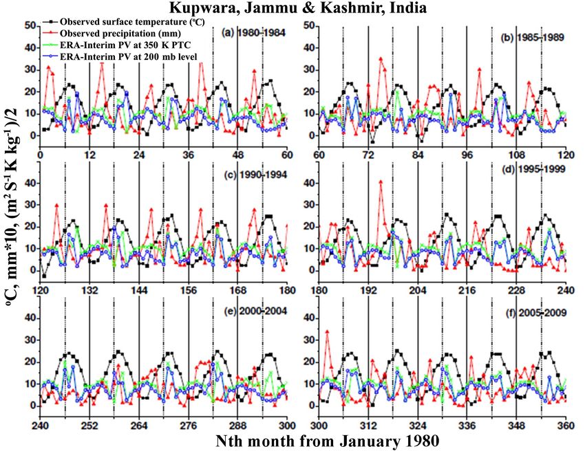
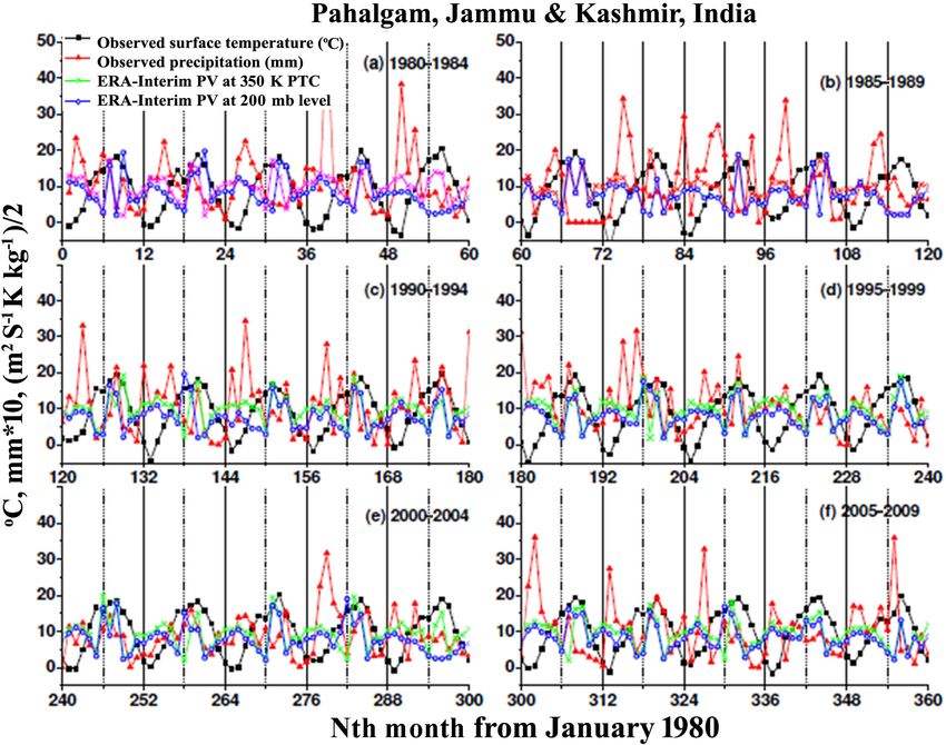
28                          S. N. Zaz et al.: Analyses of temperature and precipitation in Jammu-Kashmir for 1980–2016

Figure 10. Same as Fig. 8 but for Pahalgam.

to be significantly larger over Srinagar than other stations.     northern Kashmir region of Kupwara (Fig. 9), at mean sea
Orographic effects at other stations can have significant in-     level which is ∼ 1 km higher than Srinagar, the relation be-
fluence on planetary Rossby waves. Therefore, PV (ERA-            tween PV and precipitation is good in the years 1982–1983,
Interim data, Dee et al., 2011) in the upper troposphere varies   1985–1988, 1990–1994, 1995–1996, 1999 and 2006. Simi-
in accordance with precipitation, which is clearly depicted in    lar to Srinagar and Kokarnag, Kupwara also shows a poor
Fig. 7, during the entire years of 1984, 1987, 1988, 1990,        link during 1999–2010. Particularly during the summer mon-
1993, 1994, 1995, 1996, 1999, 2006 and 2009. Sometimes, it        soon period, the PV–precipitation relation is good in all the
is observed that the time variation of precipitation has strong   years except 1989, 1998, 2000–2005 and 2009. One inter-
correlation with PV at either 350 K surface or 200 hPa pres-      esting observation is that in 1983, 1985 and 1991 the cor-
sure surface. This would be due to the influence of Rossby        relation between PV and precipitation for Kupwara is better
waves generated due to baroclinic or and barotropic insta-        than Srinagar and Kokarnag. Since Kupwara is located near-
bilities. Particularly, the correlation between PV (sometimes     elevated Greater Himalayan mountain range, Rossby waves
either one or both) and precipitation is significantly posi-      associated with topography would have contributed to the
tive during the Indian summer monsoon months of June–             good correlation between PV and precipitation here, which
September for all the years from 1980 to 2009 except 1983,        is not the case for Srinagar and Kokarnag. In the case of Pa-
1985, 1989, 2000–2005 and 2009. At present it is not known        halgam, (Fig. 10), located near the Greater Himalayas, gen-
why this relation became weak during 1999–2010.                   erally the link between PV and precipitation is good in al-
   For Kokarnag (Fig. 8), the topography of which is similar      most all the years in the period 1980–2016 but with a differ-
to Srinagar but which is located in the vicinity of high moun-    ence that sometimes both the PVs follow precipitation and at
tains, the relation between PV and precipitation particularly     other times only one of them does. Particularly during sum-
during the Indian summer monsoon is almost similar to that        mer monsoon months, similar to Kupwara, the years 1989,
of Srinagar during 1983, 1985, 1989, 1991, 1998, 1999 and         2000–2003, 2005 and 2009 show poor correlation. In gen-
2000–2005. The deterioration of the link between PV and           eral, precipitation near the Greater Himalayas is significantly
rainfall over Kokarnag and Srinagar during 1999–2010 is in-       influenced by Rossby waves associated with topography.
triguing and it may be associated with climate change. In the

Atmos. Chem. Phys., 19, 15–37, 2019                                                  www.atmos-chem-phys.net/19/15/2019/
S. N. Zaz et al.: Analyses of temperature and precipitation in Jammu-Kashmir for 1980–2016                                    29

Figure 11. Same as Fig. 9 but for Qazigund.

   For the hilly station of Qazigund (Fig. 11), located in the    show good correlation, which is almost similar to Srinagar
south Kashmir region (above ∼ 3 km m.s.l.) near the foothills     and Kokarnag.
of Pir Panjal mountain range, the relation between PV and            In the case of Gulmarg (Fig. 12), PV and precipitation fol-
precipitation is better than that of the northern station Kup-    low each other well in the years of 1988, 1993, 1994 and
wara. For example, in 1988, the relation is much better over      1995. In 1996, during the Indian summer monsoon period of
Qazigund than Kupwara. However, the opposite is true in           June–September, only PV at 350 K surface follows precipi-
1987. Interestingly, in 1985, both Kupwara and Qazigund           tation. Overall, during the summer monsoon period, the rela-
show similar variation in PV and precipitation. This may be       tionship between PV and precipitation is appreciable for all
due to the effect of the nature of limited equatorward prop-      the years except for 1983, 1989, 1990, 1999 and 2000–2009,
agation of Rossby waves from midlatitudes. In 1995, 1997          which is almost similar to Kupwara and Pahalgam. It may be
and 1998, PV and precipitation follow similar time variation      noted that these stations are located near relatively elevated
at both Kupwara and Qazigund except for January–March             mountains and hence topographically induced Rossby waves
during which precipitation over Qazigund but not Kupwara          could have contributed to this good relation. The observa-
follows PV. Interestingly, in the whole year of 1999, precip-     tions suggest that high-altitude mountains affect the precip-
itation at both stations follows exceedingly well with PV;        itation characteristics through topography-generated Rossby
however, in 1998, only Qazigund but not Kupwara shows             waves. The interesting finding here is that irrespective of the
good relation. In 2009, precipitation does not follow PV for      different heights of mountains, all the stations show that dur-
both stations. Interestingly in all the months of 2006, PV fol-   ing 1999–2010 the correlation between upper tropospheric
lows well with precipitation for both Kupwara and Qazigund.       PV and surface precipitation was found to be poor, indicat-
However in September, Kupwara but not Qazigund shows              ing that some unknown new atmospheric dynamical concepts
good relation. In 2004, only PV at 350 K surface follows well     would have played significant role in disturbing the precipita-
with precipitation for both the stations. For the summer mon-     tion characteristics significantly over the western Himalayan
soon period of June–September, these years, namely, 1983,         region. This issue needs to be addressed in the near future by
1985, 1989, 1990, 2000–2003, 2005 and 2007–2009, do not

www.atmos-chem-phys.net/19/15/2019/                                                     Atmos. Chem. Phys., 19, 15–37, 2019
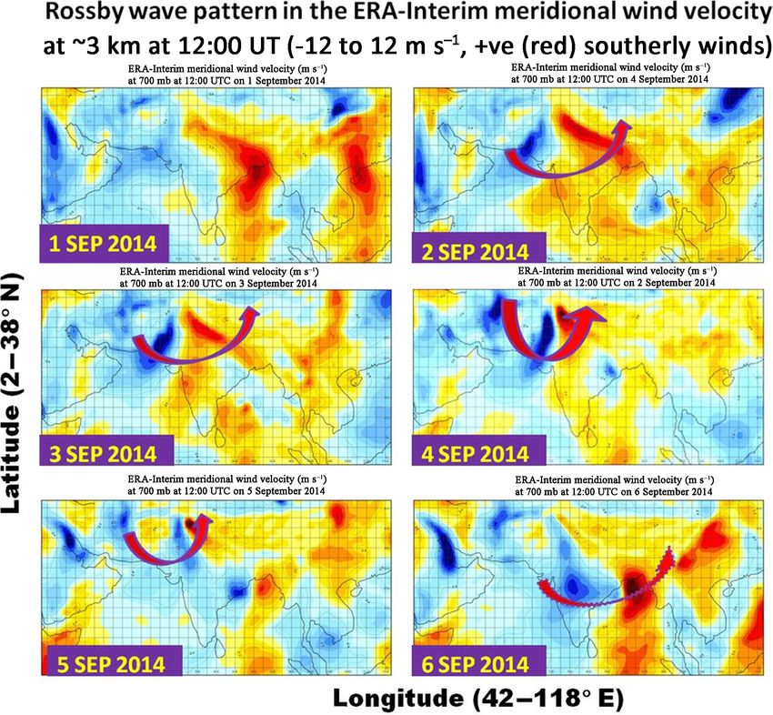
30                          S. N. Zaz et al.: Analyses of temperature and precipitation in Jammu-Kashmir for 1980–2016

Figure 12. Same as Fig. 10 but for Gulmarg.

invoking suitable theoretical models so that predictability of    2016. In the case of Kokarnag, a good relation is observed
extreme weather events can be improved in the Himalayas.          during March–August 2012, January–June 2013 and 2014,
   During 2011–2016 (Fig. 13), it may be observed that for        around September 2014. In contrast, the relationship is very
Gulmarg the link between PV and precipitation holds well          poor in the entire years of 2015 and 2016. Pahalgam interest-
in general for all these years except around July 2012, July–     ingly shows good correlation between PV and precipitation
December 2013 and 2015. It is interesting to note here that       during the whole years of 2011 and 2012. In 2013, 2014,
during the historical flood event of September 2014, the          2015 and 2016, it is good only during January–June in addi-
PV and precipitation follow each other but in the preced-         tion to being exceptionally good in September 2014.
ing and following years of 2013 and 2015 their linkage is            Finally, it may be observed that the ERA-interim reanal-
poor, as noted earlier. Similarly, all the other stations (Sri-   ysis data of meridional wind velocity (12:00 UT) at ∼ 3 km
nagar, Pahalgam, Kokarnag, Kupwara and Qazigund) also             altitude above the mean seal level show alternating positive
show that the link between PV and precipitation is good           (southerly) and negative values, resembling the atmospheric
around September 2014. This would indicate clearly that           Rossby waves in the subtropical region during 1–6 Septem-
the extreme weather event that occurred during Septem-            ber 2014 (Fig. 14). The meridional winds associated with
ber 2014 is due to intense large-scale Rossby wave activ-         Rossby waves could be easily identified to have their exten-
ity rather than any localized adverse atmospheric thermo-         sions in both the Arabian Sea and Bay of Bengal, indicating
dynamical conditions such as local convection. In Srinagar,       that water vapor from both regions was transported towards
most of the time PV and precipitation follow each other very      the Jammu and Kashmir region of India as the converging
well as observed during January 2011–June 2012, January–          point of Rossby waves was located near this region. It may be
July 2013, January–July 2014, and all of 2015 and 2016. In        easily noticed that the waves got strengthened on 4 and weak-
Qazigund, this relation is good only during January–July and      ened on 5 September and ultimately dissipated on 6 Septem-
September–October 2014 and during all of 2015 and 2016            ber. This dissipation of Rossby waves led to dumping of the
(similar to Srinagar). For Kupwara, PV follows precipita-         transported water vapor over this region and thus caused the
tion well during all of 2011, January–July 2012, January–         historical-record heavy-flooding during this period. This is
May 2013, January–November 2014, and all of 2015 and              one clear example of how synoptic-scale Rossby waves can

Atmos. Chem. Phys., 19, 15–37, 2019                                                  www.atmos-chem-phys.net/19/15/2019/
S. N. Zaz et al.: Analyses of temperature and precipitation in Jammu-Kashmir for 1980–2016                                          31

Figure 13. Same as Fig. 11 but for all the stations and during the years 2011–2016.

reorganize water vapor over large scales and lead to extreme            spheric baroclinic forcing (warming) and a stratospheric po-
rainfall events. It is well known that the subtropical westerly         lar vortex can gradually move the subtropical jet from about
jet is one of many important sources of Rossby waves in the             27 to 54◦ (Garfinkel and Waugh, 2014). Using global circu-
midlatitudes to tropical latitudes. If the subtropical jet drifts       lation models (GCMs), linear wave theory predicts that in
climatically northward then the surface weather events asso-            response to increased greenhouse gas (GHG) forcing, mid-
ciated with them also will drift similarly, leading to unusual          latitude eddy-driven jets, arising due to strong coupling be-
weather changes climatically.                                           tween synoptic-scale eddy activity and jet streams in both the
   Published reports by Barnes and Polvani (2013) and Lu et             hemispheres, will be shifted poleward (Fourth report of Inter-
al. (2014) indicate that long-term variations in Rossby wave            governmental Panel on Climate Change (IV-IPCC), Meehl et
breaking activities and stratospheric dynamics have close as-           al., 2007). However, midlatitude Rossby waves and the as-
sociation with global climate change. A meridional shift of             sociated wave dissipation in the subtropical region are pre-
the center of subtropical jets, arising due to enhanced po-             dicted to move climatologically towards the equator due to
lar vortex and upper-tropospheric baroclinicity, is possible            the spherical geometry of the Earth (Hoskins et al., 1977; Ed-
due to the consequences of global warming, has been suc-                mon et al., 1980). This propagation of the location of wave
cessfully linked to climatic changes in Rossby wave break-              breaking towards the equator will have a long-term (climatic)
ing events caused by baroclinic instabilities (Wittman et al.,          impact on the relation between variations in upper tropo-
2007; Kunz et al., 2009; Rivière, 2011; Wilcox et al., 2012).           spheric PV associated with Rossby waves and surface pre-
The long-term increase in the tropospheric warming arising              cipitation in the subtropical latitude regions. This may be one
due to baroclinic forcing of Rossby waves is more promi-                of the reasons that during 1999–2010, the relation between
nent in the midlatitudes than in the tropical regions (Allen            PV and precipitation became poor, as observed in the present
et al., 2012; Tandon et al., 2013). This midlatitude warming            study.
plays a critical role in driving poleward shifts of the subtrop-           Regarding surface temperature, except for its linear long-
ical jet responding to climate change (Ceppi et al., 2014).             term trend, there is no clear evidence of a strong link between
It should be remembered that the combined effect of tropo-              variations in the upper tropospheric potential vorticities and

www.atmos-chem-phys.net/19/15/2019/                                                           Atmos. Chem. Phys., 19, 15–37, 2019
You can also read