Enhancing Precipitation Estimates Through the Fusion of Weather Radar, Satellite Retrievals, and Surface Parameters
←
→
Page content transcription
If your browser does not render page correctly, please read the page content below
remote sensing
Article
Enhancing Precipitation Estimates Through the
Fusion of Weather Radar, Satellite Retrievals, and
Surface Parameters
Youssef Wehbe 1,2, * , Marouane Temimi 1 and Robert F. Adler 3
1 Department of Civil Infrastructure and Environmental Engineering, Khalifa University of Science and
Technology, P.O. Box 54224, Abu Dhabi, UAE; marouane.temimi@ku.ac.ae
2 National Center of Meteorology (NCM), P.O. Box 4815, Abu Dhabi, UAE
3 Earth System Science Interdisciplinary Center, University of Maryland, College Park, MD 20740, USA;
radler@umd.edu
* Correspondence: ywehbe@ncms.ae
Received: 5 February 2020; Accepted: 8 April 2020; Published: 23 April 2020
Abstract: Accurate and timely monitoring of precipitation remains a challenge, particularly in
hyper-arid regions such as the United Arab Emirates (UAE). The aim of this study is to improve
the accuracy of the Integrated Multi-satellitE Retrievals for the Global Precipitation Measurement
(GPM) mission’s latest product release (IMERG V06B) locally over the UAE. Two distinct approaches,
namely, geographically weighted regression (GWR), and artificial neural networks (ANNs) are
tested. Daily soil moisture retrievals from the Soil Moisture Active Passive (SMAP) mission (9 km),
terrain elevations from the Advanced Spaceborne Thermal Emission and Reflection digital elevation
model (ASTER DEM, 30 m) and precipitation estimates (0.5 km) from a weather radar network are
incorporated as explanatory variables in the proposed GWR and ANN model frameworks. First,
the performances of the daily GPM and weather radar estimates are assessed using a network of
65 rain gauges from 1 January 2015 to 31 December 2018. Next, the GWR and ANN models are
developed with 52 gauges used for training and 13 gauges reserved for model testing and seasonal
inter-comparisons. GPM estimates record higher Pearson correlation coefficients (PCC) at rain gauges
with increasing elevation (z) and higher rainfall amounts (PCC = 0.29 z0.12 ), while weather radar
estimates perform better for lower elevations and light rain conditions (PCC = 0.81 z−0.18 ). Taylor
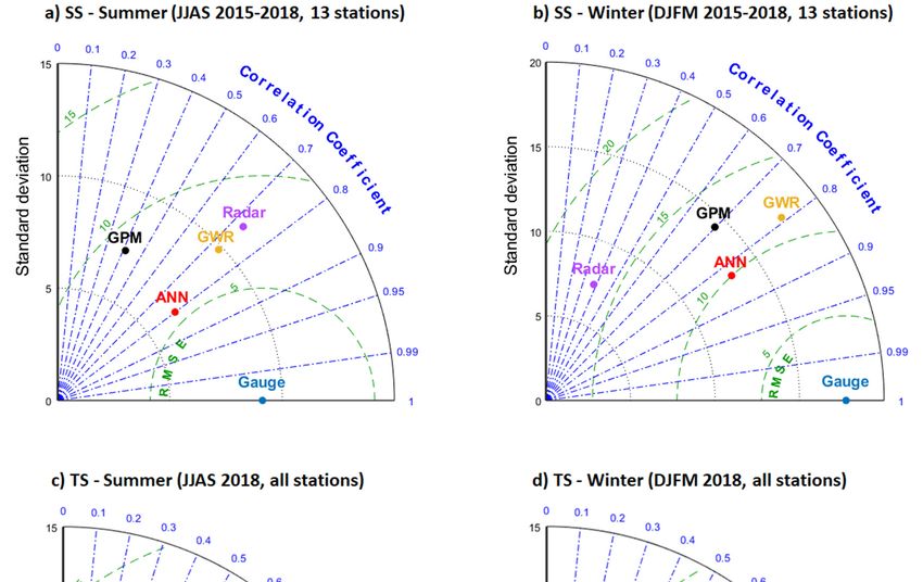
diagrams indicate that both the GWR- and the ANN-adjusted precipitation products outperform the
original GPM and radar estimates, with the poorest correction obtained by GWR during the summer
period. The incorporation of soil moisture resulted in improved corrections by the ANN model
compared to the GWR, with relative increases in Nash–Sutcliffe efficiency (NSE) coefficients of 56%
(and 25%) for GPM estimates, and 34% (and 53%) for radar estimates during summer (and winter)
periods. The ANN-derived precipitation estimates can be used to force hydrological models over
ungauged areas across the UAE. The methodology is expandable to other arid and hyper-arid regions
requiring improved precipitation monitoring.
Keywords: precipitation; artificial neural networks; geographically weighted regression; weather
radar; soil moisture
1. Introduction
Despite the widely reported inconsistencies of precipitation products over the Arabian
Peninsula [1–4], a limited number of studies have attempted to improve precipitation monitoring
over the progressively water-stressed region. Existing attempts are limited to gauge-based bivariate
linear regression approaches [5,6]. Sources of precipitation estimates can be broadly grouped into
Remote Sens. 2020, 12, 1342; doi:10.3390/rs12081342 www.mdpi.com/journal/remotesensing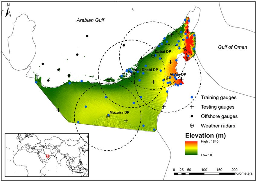
Remote Sens. 2020, 12, 1342                                                                          2 of 28

three classes, namely: (i) ground-based rain gauge and radar observations, (ii) satellite precipitation
retrievals, and (iii) reanalysis products fused from numerical weather predictions (NWP) models and
observations. Despite the ongoing leaps in computational power, several key processes like convection,
phase change, and collision–coalescence occur at the microscale, i.e., nine orders of magnitude less
than current weather or climate model resolutions [7].
      Remotely sensed precipitation estimates from ground-based radar and satellite platforms offer
an attractive alternative to reanalysis products due to their higher spatiotemporal resolutions and
coverage. Weather radars generate high-resolution real-time estimates of rainfall above the surface
by emitting electromagnetic signals and analyzing backscatters from intercepted hydrometeors [8].
Consequently, the reliability of radar rainfall estimates is diminished by several factors, such as terrain
blockage, different sources of clutter and signal attenuation [9,10]. Additionally, the high maintenance
costs associated with weather radars limit their deployment at the global scale. With their global
coverage, satellite products continue to be the most widely used precipitation data sources. These
include products from the Tropical Rainfall Measurement Mission (TRMM) [11] and its successor
the Global Precipitation Measurement (GPM) mission [12], the Global Precipitation Climate Center
(GPCC) [13], the Climate Research Unit (CRU) [14], and the Climate Prediction Center morphing
(CMORPH) technique [15], among others. Despite their widespread applications, their uncertainties
remain high, especially over arid regions with absolute and relative biases reaching 100 mm and 300%,
respectively [16,17]. The sparse distribution of rain gauges and inhomogeneity of observations hamper
the calibration of such products for improved water resource management with rapidly expanding
urbanization across the Arabian Peninsula [5].
      To ameliorate the uncertainties, both precipitation correction and multi-source estimation
approaches have been explored and applied for different regions. Here, we distinguish between (1) the
conventional approach of exclusively relying on rain gauge observations [6,18,19] and (2) the more
recent approach of incorporating additional explanatory variables [20–23] to correct precipitation
estimates. The latter approach is the focus of the current study. A physically-based selection of
explanatory variables is expected to preserve process dynamics and interlinkages within datasets
which remain unresolved in conventional statistical correction methods. For example, water content
in the uppermost soil layer exhibits an instantaneous response to collocated precipitation and is
widely used as a proxy for precipitation occurrence. In fact, most currently used soil moisture
retrieval algorithms are corrected by precipitation flags (rain/no rain) from available precipitation
sources [24–26]. This soil moisture–precipitation dependency is particularly relevant for arid regions
and desert environments, where background/residual soil moisture prior to a rain event is relatively
uniform as a result of negligible surface flow. Therefore, any soil moisture perturbations are controlled
by the spatiotemporal distribution of rainfall events and provide a sustained surface signature beyond
the satellite overpass time. Using the Weather Research and Forecasting (WRF) model, Weston, et al. [27]
studied the sensitivity of the heat exchange coefficient to surface conditions, including soil moisture,
and demonstrated a strong impact on heat fluxes and local meteorological conditions within the
United Arab Emirates (UAE). Elevation is another explanatory variable that has been widely used for
precipitation correction [28–31] and is especially relevant to the current study area, given the frequently
occurring local orographic rainfall events over the northeastern UAE [32–34]. Additional surface and
atmospheric variable inputs, such as slope, air temperature, vegetation indices, surface energy fluxes
and cloud characteristics have been investigated [35]. The significance of the selected inputs varies
based on the geographic and climatic attributes of each study domain and, more importantly, based on
the methodology followed.
      Several studies report spatial correlations between precipitation and vegetation indices [36],
topography [37], and land surface temperature [38]. It is crucial to account for all possible explanatory
variables in the estimation of precipitation. In this regard, the geographically weighted regression
(GWR) method has proven to be reliable, especially for precipitation product correction and
downscaling [29,30,39]. Initially proposed by Brunsdon, et al. [40], GWR was developed to infer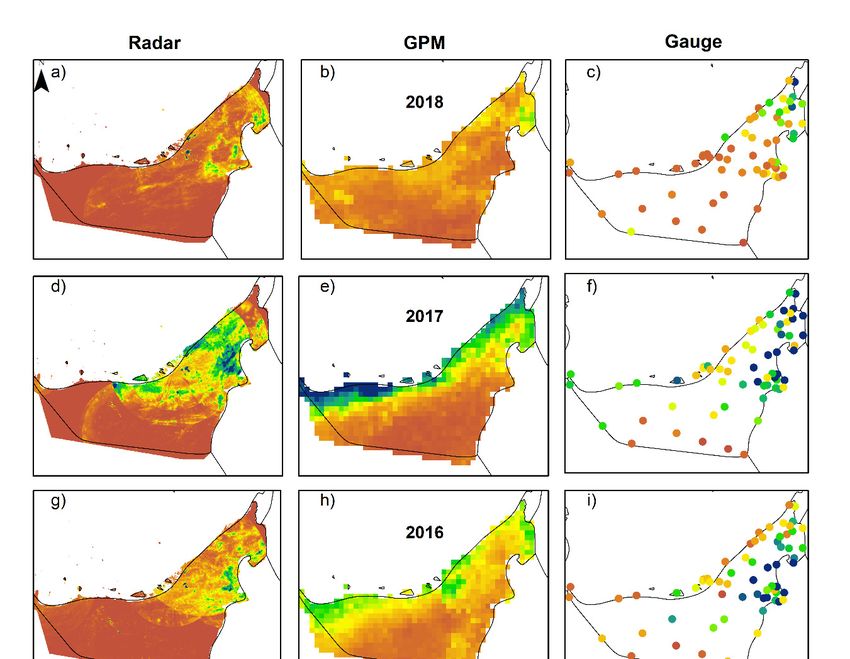
Remote Sens. 2020, 12, 1342                                                                          3 of 28

spatially varying dependencies between datasets beyond the simplifying assumption of constant
relationships in space imposed by linear regression [41]. Using a GWR model, Kamarianakis, et al. [42]
tested the hypothesis of null spatial non-stationarity in the relationship between rain gauge observations
and collocated satellite estimates over the Mediterranean. Rejecting the null hypothesis, they found
statistically significant spatial non-stationary components, with the satellite algorithm performing
better in geographical locations with specific terrain attributes. Chao et al. [35] used a GWR-based
approach to merge daily CMORPH precipitation with gauge records over the Ziwuhe Basin of China.
They incorporated additional surface inputs, namely, slope, aspect, surface roughness, and distance to
coastline in their model. Compared to the original CMORPH estimates, their merged product improved
the gauge-based correlation from 0.208 to 0.724, and RMSE from 1.208 to 0.706 mm/hr. Relevant
to the current study area, Wehbe et al. [3] conducted the first attempt to assess the consistency of
different precipitation products over the Arabian Peninsula. They employed geographically-temporally
weighted regression to infer water storage variations from inputs of soil moisture, terrain elevation
and four different precipitation datasets. The TRMM Multi-Satellite Precipitation Analysis (TMPA V7)
product showed the best predictive performance with a goodness-of-fit coefficient (R2 ) of 0.84.
      Blending explanatory variables to enhance precipitation estimates has also been addressed using
Artificial Neural Networks (ANNs), a subset of machine learning (ML) techniques, that have been
increasingly applied in climate studies for their abilities to perform adaptive, efficient, and holistic
mappings of nonlinearities between large datasets [43,44]. Maier, et al. [45] and Gopal [46] give a detailed
overview on the development and application of ANNs and their most compatible configurations
for geospatial analyses. While several types of ANNs have been developed for different applications,
the feedforward multilayer perceptron (MLP) architecture remains the most commonly used framework
for modeling precipitation [47–51]. In addition to model- and satellite-based precipitation correction
attempts, ANNs have also been successfully applied to improve weather radar rainfall estimates [52–56].
Moghim et al. [18] applied a three-layer feedforward neural network to correct precipitation and
temperature model outputs over northern South America. For precipitation correction, they obtained
consistent improvements of 8%, 8.5%, and 15.7% in mean square error, bias, and correlation metrics,
respectively from the ANN configuration compared to linear regression. On the other hand, without
incorporating precipitation inputs, Fereidoon and Koch [22] trained an ANN with daily inputs from the
Advanced Microwave Scanning Radiometer - Earth Observing System (AMSR-E) soil moisture product
and air temperature measurements against rainfall records at five weather stations. Nevertheless,
the ANN performed reasonably well with R2 values reaching 0.65 during testing. Importantly, despite
using separate time periods, they locally tested their model at the same stations used for training
without attempting to verify the generalized spatial performance of the ANN-based estimates. They
also highlighted the need for further case studies to be conducted over other regions with different soil
moisture products.
      This study provides the first attempt of multivariate nonlinear precipitation estimation over the
UAE by correcting the Integrated Multi-satellitE Retrievals for the Global Precipitation Measurement
(GPM) mission’s latest daily product release (IMERG V06B) overland using ancillary data and
explanatory variables. Two techniques are tested, namely, the GWR and the ANN. First, to assess
multi-collinearity of the datasets, the individual performances of both GPM and ground-based radar
precipitation estimates are compared against 65 rain gauge records from 1 January 2015 to 31 December
2018. Next, the proposed configuration and development of the GWR and ANN models using 52
out of the 65 available rain gauges is outlined. In addition to the GPM and radar estimates, terrain
elevation, and satellite soil moisture estimates are used as explanatory variables to incorporate surface
wetting signatures. Finally, both models are inter-compared to the original GPM and radar estimates
at 13 gauges left out during the training process. The developed models are expected to outperform
both the GPM and radar estimates by overcoming their individual biases.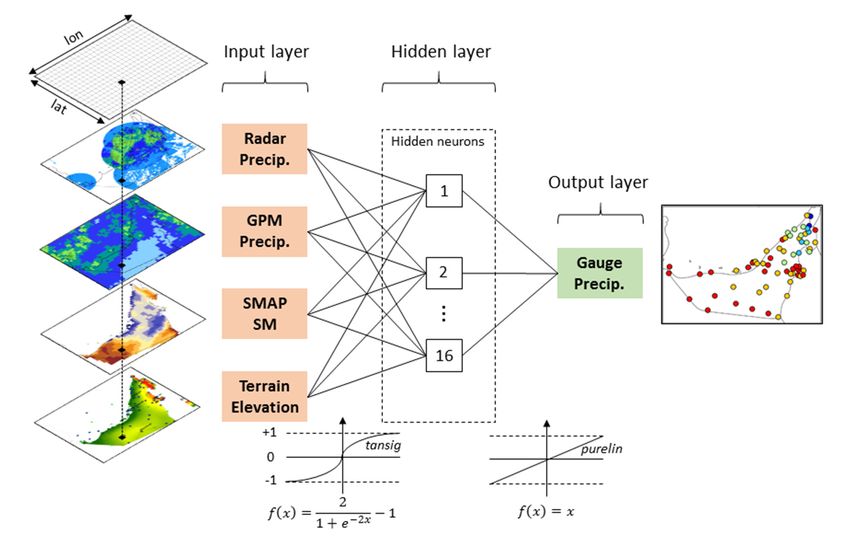
Remote Sens. 2020, 12, 1342 4 of 28
Remote Sens. 2020, 12, x FOR PEER REVIEW 4 of 28
2.2.Materials
Materials
2.1.
2.1.Rain
RainGauge
GaugeData
Data
Figure
Figure11shows
showsthetheUAE
UAEstudystudyarea
areaand
andtopography
topographyderived
derivedfrom
fromthe
theAdvanced
AdvancedSpaceborne
Spaceborne
Thermal Emission and Reflection Radiometer (ASTER) digital elevation model (DEM),
Thermal Emission and Reflection Radiometer (ASTER) digital elevation model (DEM), described describedin
in Toutin [57]. Ground-based rainfall observations are recorded from a network of
Toutin [57]. Ground-based rainfall observations are recorded from a network of 72 rain gauges72 rain gauges(7
(7offshore
offshoreand
and6565overland)
overland)operated
operatedby bythe
theUAE
UAE National
National Center
Center of
of Meteorology
Meteorology (NCM).
(NCM).TheThetraining
training
and testing stations used for the model development are also indicated. While rainfall
and testing stations used for the model development are also indicated. While rainfall amounts amountsare
are logged
logged at at 15-min
15-min intervalsbybythe
intervals thegauges,
gauges,the
the quality-controlled
quality-controlled daily
daily accumulations
accumulations were
were made
made
available
availablefor
forthis
thisstudy.
study.
Figure1.1. Terrain
Figure Terrain elevation
elevation map
map derived
derived from
from the
the ASTER
ASTER DEMDEM forfor the
theUAE
UAEstudy
studydomain
domainwith
with
locationsofofrain
locations raingauges
gauges(7(7offshore
offshoreand
and65
65overland:
overland:5252for
fortraining
trainingand
and13 13for
fortesting)
testing)and
andthe
theweather
weather
radarnetwork.
radar network.
The
Theseven
sevenoffshore
offshoregauges are not
gauges areused
not in the current
used work since
in the current the correction
work since the would be exclusively
correction would be
gauge-based due to the limited
exclusively gauge-based due extent
to the of the radar
limited estimates
extent of theand theirestimates
radar additional uncertainties
and from
their additional
sea clutter. Thefrom
uncertainties offshore univariate
sea clutter. Thecorrection approach would
offshore univariate require
correction a simpler
approach wouldmodel configuration
require a simpler
(e.g.,
model ordinary least squares
configuration regression),
(e.g., ordinary assquares
least pursuedregression),
in [5] for the
as TMPA
pursuedV7inproduct
[5] for over the same
the TMPA V7
study
productarea. More
over theimportantly, the limited
same study area. number of offshore
More importantly, gauges
the limited requireofaoffshore
number longer study
gaugesperiod to
require
ensure representative results which are reserved for future work.
a longer study period to ensure representative results which are reserved for future work.
2.2.
2.2.Radar-Based
Radar-based Rainfall
Rainfall Estimates
Estimates
Figure
Figure 11 also
also shows
shows the
thelocations
locationsofofthethe NCM
NCM weather
weather radar
radar network,
network, composed
composed of dual-
of four four
dual-polarization
polarization radars deployed in Abu Dhabi, Al Ain, Dubai, and Muzaira. All radars operate in the in
radars deployed in Abu Dhabi, Al Ain, Dubai, and Muzaira. All radars operate C-
the C-band with the following specifications:
band with the following specifications:
• Instrumented range: 200 km
• Range gate: 100 m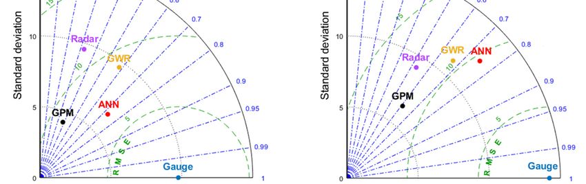
Remote Sens. 2020, 12, 1342                                                                           5 of 28

•     Instrumented range: 200 km
•     Range gate: 100 m
•     Min-Max elevation angles: 0.5◦ –32.4◦
•     3-dB-Beamwidth: 1◦
•     Time interval of volume scans: 6 min

     The Thunderstorm Identification Tracking and Analyses (TITAN) software [58], which is included
in the Lidar Radar Open Software Environment (LROSE), is used for the operational radar data
processing. Default algorithms and correction factors are used for de-cluttering, noise filtering and
attenuation correction. A fuzzy logic classifier is applied for de-cluttering using the features of: radial
velocity, texture of reflectivity, texture of differential reflectivity, and correlation coefficient. This is
followed by noise filtering by a moving average window. Next, a standard C-band attenuation
correction factor (ACF) of 0.014 dB per degree is applied based on the approximated linear relationship
between specific (and differential) attenuation and differential phase [59]. Finally, the merged plan
position indicator (PPI) is used to merge multiple radar overlaps based on a maximum reflectivity
value approach. The radars are subject to annually-scheduled calibrations by the manufacturer using
the dual-pol measurements, as well as routine maintenance to maintain a ±1 dB error margin.
     The Z−R relation used for rainfall estimation is set by the manufacturer as Z = 200 R1.455 (adapted
from [60]) for mixed-phase cloud processes typical to the UAE. At a range limit of 100 km (outlined in
Figure 1), the rainfall intensity R (mm/hr) is estimated for each 6-min, 100-m (range gate) elemental
volume scan using vertical levels between 1–3 km. The rainfall amounts are then accumulated to the
daily timescale and re-gridded to the 0.5 km resolution provided to the authors. It is important to note
the range-dependent variations in the elemental volume scan resolution, where beam widths sampled
at ranges beyond ~30 km exceed the 0.5 km resolution used here. Evaporative loss below the 1 km
level is not corrected for, and no gauge data is used for calibration/validation.
     Apart from the aforementioned quality control steps for the radar data, bias-correction using the
gauge observations would prevent the use of the radar data in the multivariate approach sought here.
Data pre-processing (Section 3) involves further steps to reduce the impact of remaining data quality
issues on the training and model performance. Uncertainties from the aforementioned standard quality
control steps remain, but may favor the generalization of model correction performance during the
training stage [61]. On the other hand, pronounced errors may exist over the northeastern highlands
due to terrain blockage and merging uncertainties. The authors intend to assess different gap-filling
methods to improve coverage for this area in separate work.

2.3. GPM IMERG (Version 06B) Precipitation Product
     The GPM mission, launched in February 2014, provides higher resolution (30-min, 0.1◦ )
precipitation estimates through the IMERG product, compared to its TRMM TMPA (3-hourly, 0.25◦ )
predecessor. The IMERG algorithm inter-calibrates, merges and interpolates GPM constellation satellite
precipitation estimates with microwave-calibrated infrared estimates and rain gauge analyses to produce
a higher resolution and more accurate product [12]. The GPM core satellite estimates precipitation
from two instruments, the GPM microwave imager (GMI) and the dual-frequency precipitation radar
(DPR). More importantly for this study, the DPR adds sensitivity to light precipitation, compared to
that of TRMM’s single-frequency radar. The latest release V6 uses an improved morphing scheme
with a model-based propagation from the Modern-Era Retrospective analysis for Research and
Applications, Version 2 (MERRA-2), compared to the V5 satellite-based propagation vectors of IR
cloud-top temperature.
     The GPM IMERG V06B Level-3 (L3) daily product without gauge correction is used to ensure no
prior dependencies on the rain gauge data as ground truth. Nevertheless, the gauges used here are not
included in the World Meteorological Organization’s Global Precipitation Climatology Network which
is used for the final IMERG calibration [62].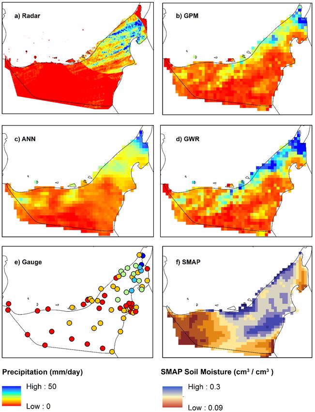
Remote Sens. 2020, 12, 1342                                                                           6 of 28

2.4. SMAP Enhanced L3 (Version 2) Soil Moisture Product
     On 31 January 2015, NASA launched the SMAP mission as the first attempt to collect coincident
measurements of active (radar) and passive (microwave) soil moisture retrievals [63,64]. Up to 5 cm
depth of soil moisture is estimated on a 685-km, near-polar, sun-synchronous orbit, with equator
crossings at 6:00 a.m. (descending) and 6:00 p.m. (ascending) local time. However, a permanent fault
in the radar instrument on 7 July 2015 left only the radiometer-derived and assimilated soil moisture
estimates. To compensate for the active retrieval loss, the European Space Agency’s Sentinel-1A and
-1B C-band radar backscatter coefficients were incorporated to derive the L2 SMAP soil moisture
product. The enhanced L3 soil moisture product used here is a daily composite of the L2 soil moisture
gridded on a 9-km Equal-Area Scalable Earth Grid, Version 2.0 (EASE-Grid 2.0) in a global cylindrical
projection. Both the ascending and descending overpasses are used here for the daily estimates, with
the higher pixel values retained in case of overlaps.

3. Methods
     In this section, the proposed GWR model configuration and ANN architecture, along with
their respective training approaches are presented. Then, the k-fold cross-validation method [65]
used for model calibration is outlined. Finally, the statistical metrics and testing approach used for
inter-comparing model performances are presented.
     The daily GPM estimates are available at 0.1◦ × 0.1◦ grid scales. Consequently, data pre-processing
involved aggregating the weather radar (0.5 km), SMAP (9 km) and ASTER (30 m) datasets to
consistent 0.1◦ (see Figure A1 in Appendix A) and daily resolutions for model training and testing.
The statistical significance of each of the considered input predictors is assessed using ordinary least
squares regression. The t-test [66] hypothesis testing is adopted as a widely used method to identify
and sort predictors among a pool of independent variables [28]. Additionally, the Pearson correlation
coefficient (PCC) is used to test independent variables for multi-collinearity [67]. Removing covariates
that are highly correlated is suggested to avoid standard errors and biases in a regressive model [68].
All four selected predictors showed to be statistically significant with p-values less than 0.001 and low
multi-collinearity potential with all pair-wise PCCs < 0.5.
     A detailed sensitivity analysis of the impact of input data quality on predictive accuracy for an
ANN with a single hidden layer is reported in [69]. A significant decrease in model performance is
recorded for data error rates beyond 20% during the training stage, compared to the base case scenario
with unperturbed training data. However, the model performance slightly improves as the input data
error rate varies between 5–15%. This is consistent with other findings showing that the involved
arithmetic operations can dampen random and systematic errors in input data. Pre-processing involved
normalizing all datasets to zero mean and unity standard deviation distributions (i.e., ranging between
−1 and 1) for faster convergence [70,71]. The model outputs are then de-normalized and returned to the
original form. Details on the normalization and de-normalization steps can be found in Appendix A.

3.1. GWR Model Configuration
     Precipitation is typically characterized by large spatial variability, which is especially the case for
the UAE’s rainfall regime. As such, inferring weighted relationships irrespective of spatial information
(using all pixels) through global regression methods introduces significant bias. Local methods such as
GWR are proposed to account for spatial non-stationarity by assigning variable weights at selected
locations (pixel-per-pixel). Equation (1) illustrates the generalized form of the GWR model proposed
by Brunsdon et al. [40].
                                                     X
                              Yi = βo (ui , vi ) +       βk (ui , vi )Xik + εi i = 1, . . . , n          (1)
                                                     k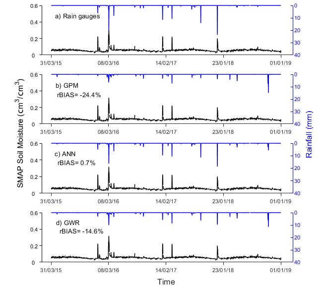
Remote Sens. 2020, 12, 1342 7 of 28
where Yi denotes the ith observation of the dependent variable, βo (ui , vi ) is the intercept value at the
geographical location (ui , vi ), βk (ui , vi ) is the set of coefficient weights at each location for k independent
variable (predictor) values Xi , and εi is the aggregated residual term. The detailed derivation of
Equation (1) and the GWR approach in general is provided by Brunsdon, et al. [72].
For the special case of βk (u1 , v1 ) = βk (u2 , v2 ) = . . . = βk (un , vn ), Equation (1) can be reduced to
a simple linear regression equation. The coefficient weights for the ith observation can be expressed
(without the spatial coordinates ui and vi ) as
−1
β̂i = XT Wi X XT Wi Y (2)
where Wi is a matrix (n × n) with a diagonal of coefficient weight elements. The Gauss function is
used between observations i and regression point j to provide a continuous and exponential decay
relationship between the distance function and the weighting matrix as
dij 2
Wij = exp − 2 (3)
b
where b is the Gaussian kernel bandwidth and dij denotes the distance function. Given the
uneven distribution of stations, an adaptive bandwidth b is automatically assigned based on
cross-validation [73,74]. The developed GWR model can be expressed as
CPi = βo (ui , vi ) + β1 (ui , vi )RPi + β2 (ui , vi )SPi + β3 (ui , vi )SMi + β4 (ui , vi )Zi + εi (4)
where CPi is the corrected precipitation output, RPi and SPi are the ground-based radar and satellite
precipitation, respectively, SMi is the SMAP soil moisture estimate and Zi is the ASTER DEM value,
each at any point (ui , vi ) across the domain at 0.1◦ resolution.
When time-dependent relationships are expected between input and/or output variables,
time-varying weights must be derived. For example, geographically-temporally weighted regression
was used by the authors to investigate rainfall-groundwater recharge mechanisms in previous work [3].
However, in the current study, a same-day response is expected between the input and output datasets
(i.e., any change in observed rainfall will reflect on both radar and satellite estimates, as well as on soil
moisture at the daily scale). Therefore, spatially distributed weights from GWR are used here without
temporal variation.
3.2. ANN Architecture
3.2.1. Feedforward MLP Configuration
ANNs can simulate complex nonlinear relationships between variables and resolve higher-order
dependencies overlooked by conventional linear regression methods. ANNs were formulated to
replicate the functionality and learning ability of biological neural networks, with neurons being their
basic functional units. Each neuron is bounded by input and output variables, with intermediary
weighting coefficients and activation functions embedded in one or more hidden layers. The widely
used feedforward MLP architecture is a type of supervised ANN that requires output information
(targets) to be specified. The configuration of a feedforward MLP is defined by the number of hidden
layers and hidden neurons as well as the selected activation functions and training algorithms.
Table 1 gives an overview of the proposed MLP configuration and reasoning for each selection.
One hidden layer is chosen according to the widely recommended three-layer feedforward network
configuration [44,46], particularly for precipitation bias correction studies as sought here [18,47,75].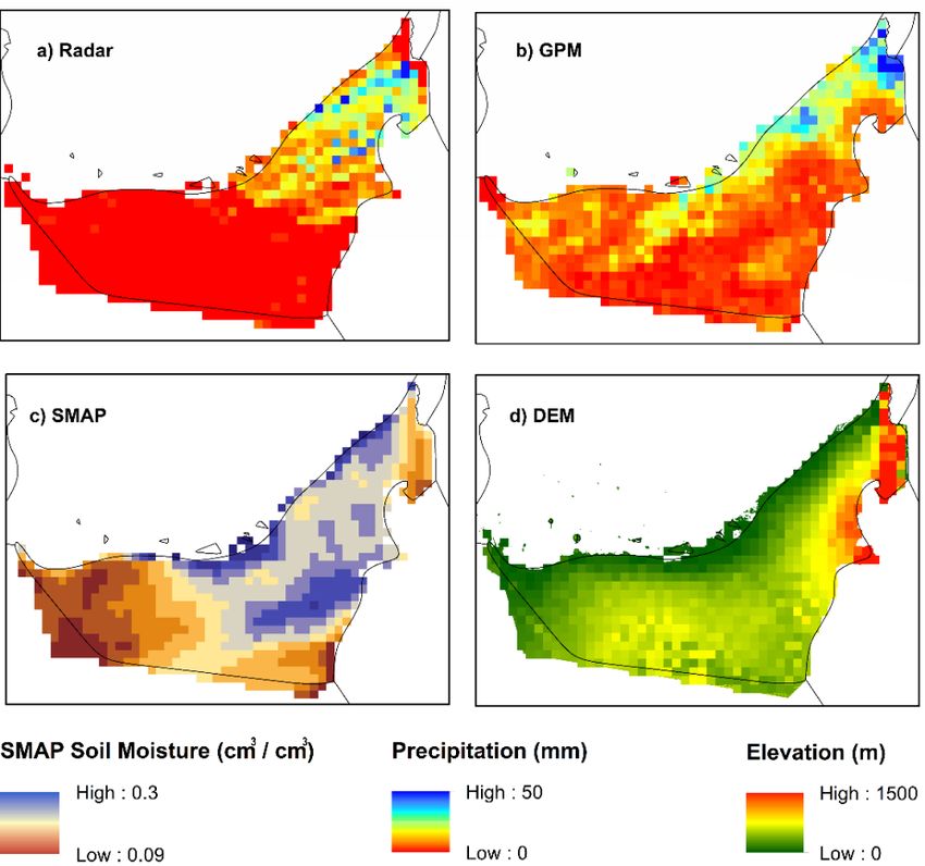
Remote Sens. 2020, 12, 1342 8 of 28
Table 1. Overview of selected configuration and parameter values for the proposed ANN.
Network Attribute Value/Selection Reasoning
No. of hidden layers 1 See [18,47,75]
No. of hidden neurons (n) 16 From 10-fold cross-validation [76]
Hidden and output layer activation Hyperbolic tangent (tansig) and linear
See [18,77]
functions (purelin) transfers
Training algorithm Levenberg–Marquardt algorithm (trainlm) See [18,71]
Activation functions, also known as transfer functions, provide sequential connections between
neurons in all three layers. First, the input data is weighted and forwarded to the hidden layer where
the weighted summations are then converted to output fields. Sigmoid-based functions are reported
to be the most applied functions between the input and hidden layers [79,80]. Depending on the
application, selected types of activation functions (including sigmoid subtypes) are known to improve
the performance of ANNs, but do not constrain the networks’ mapping power [81]. The hyperbolic
tangent (tansig) and linear (purelin) transfer functions are selected here for the hidden and output
layers, respectively, due to their reported success when used for precipitation bias correction [18,77].
Following the same terminology used for Equation (5) and without explicit listing of spatial coordinates
(ui , vi ), the general form of the proposed MLP can be expressed as
Xn
CPi = fout λj fhid βjo + βj1 RPi + βj2 SPi + βj3 SMi + βj4 Zi + βo (5)
j=1
where n is the number of hidden neurons, λj are the connection weights between the jth neuron in the
hidden layer and the output neuron, βj1 , βj2 , . . . βj4 are the connection weights between the jth neuron
of the hidden layer and each of the four neurons of the input layer, βjo and βo are the bias parameters,
and fout and fhid are the activation functions for the output and hidden layers, respectively.
3.2.2. Training Algorithm
As in the case of GWR, weights are the key parameters of the MLP determined by a selected
training algorithm. A training algorithm continuously modifies the network’s weights and biases with
the aim of minimizing a predefined error function (mean squared error used here) between the gauge
observations and network output. The choice of the training algorithm dictates the computation time
for the training and, consequently, the memory capacity, especially with a large number of inputs.
The Levenberg–Marquardt (LM) algorithm [82] combines the advantages of both the Gauss–Newton
(GN) [83] and the gradient descent (GD) methods [84] in terms of fast convergence with randomly
assigned initial weights. This dictates its widespread use for training moderate-sized networks with
up to several hundred weights [78,85–87].
The detailed derivation of the LM method can be found in Marquardt [88]. Similar to the Newton
methods, the LM avoids the costly computation of the Hessian matrix, expressed as H = JT J and
gradient g = JT e, where J is the Jacobian matrix that contains first derivatives of the network errors with
respect to the weights and biases, and e is a vector of the network errors. A standard backpropagation
technique is used to compute the Jacobian matrix in place of the Hessian matrix, and the LM algorithm
can be expressed as
−1
wk+1 = wk − JTk Jk + µI g (6)
where wk is the vector of weights for the kth iteration, I is the identity matrix, and µ is a nonzero
combination coefficient that ensures the Hessian matrix is invertible. For larger and smaller values of
µ, the LM method approaches the GD and GN methods, respectively.
The dimension of the hidden weight matrix is 4 × 16, where each input variable is associated
with 16 weights (one per hidden neuron) followed by a 16 × 1 output weight matrix. The neurons
are adaptively activated depending on the data fed to the network. This complexity is expected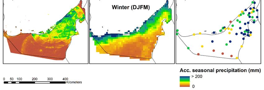
Remote Sens. 2020, 12, 1342 9 of 28
to preserve hidden information (including spatial) when trained with the gauge observations and
collocated variables [46].
Figure 2 illustrates the proposed configuration of the feedforward MLP with an input layer
consisting of 4 neurons, a hidden layer with 16 neurons, and an output layer consisting of 1 neuron,
as well as the selected activation functions. Details on the MLP calibration by k-fold cross-validation
can beSens.
Remote found2020,in12,Appendix
x FOR PEERA.
REVIEW 9 of 28
Figure
Figure 2.
2. Architecture
Architecture of
of the
the proposed
proposed feedforward
feedforward MLP
MLP with
with an
an input
input layer
layer consisting
consisting of
of 44neurons,
neurons,
aa hidden
hidden layer of 16 neurons, and an output layer of 1 neuron. The two intermediary activation
layer of 16 neurons, and an output layer of 1 neuron. The two intermediary activation
functions (tansig and purelin) are displayed below their mapping stage.
3.3. Model
3.3. Model Testing
Testing and
and Skill
Skill Scores
Scores
The 4-year
The 4-year (2015–2018)
(2015–2018) annual
annual average
average rainfall
rainfall was
was computed
computed for for each
each of
of the
the 65
65 gauges
gauges and
and
ascendingly ranked.
ascendingly ranked. Then,
Then, aa verification
verification (testing)
(testing) station
station was
was sequentially
sequentially selected
selected for
for every
every 55 ranks,
ranks,
amounting to 13 stations. The remaining 52 stations were used for training. This
amounting to 13 stations. The remaining 52 stations were used for training. This approach captures approach captures the
domain’s full precipitation range [89]. The number of testing gauges (13) was
the domain’s full precipitation range [91]. The number of testing gauges (13) was determined as 20% determined as 20% of
thethe
of total 65 65
total gauges.
gauges.This is is
This in in
line with
line withthethe
commonly
commonly used
used80/20
80/20ratio forfor
ratio training/testing
training/testingsamples
samples to
ensure proper verification without compromising the training quality [90].
to ensure proper verification without compromising the training quality [92]. Figure 1 Error! Figure 1 shows the spatial
distributionsource
Reference of the training and testingthe
not found.shows gauges.
spatialAndistribution
alternative approach is temporal
of the training sub-setting
and testing (TS)An
gauges. by
using the full
alternative networkisoftemporal
approach stations for training during
sub-setting (TS) by2015–2017,
using the fullandnetwork
testing during 2018.for training
of stations
After training and calibration,
during 2015–2017, and testing during 2018. the GWR and ANN models are tested over an independent
subsample using both
After training andspatial and temporal
calibration, the GWR divisions.
and ANN The error
models measures usedover
are tested are listed below and
an independent
include the root mean squared error (RMSE), relative BIAS (rBIAS), probability
subsample using both spatial and temporal divisions. The error measures used are listed below of detection (POD) and
and
false alarm ratio (FAR). A threshold of 3 mm was used for computing the POD
include the root mean squared error (RMSE), relative BIAS (rBIAS), probability of detection (POD) and FAR values as
recommended
and false alarminratio
[5]. (FAR). A threshold of 3 s mm was used for computing the POD and FAR values
Pn 2
as recommended in [5].
i=1 yest i − yoi
RMSE = (7)
n
∑ (y −y )
RMSE = (7)
n
∑ (y −y )
rBIAS = (8)
∑ y
events detected by both rain gauge and estimate source
POD = (9)
events detected by rain gauge alone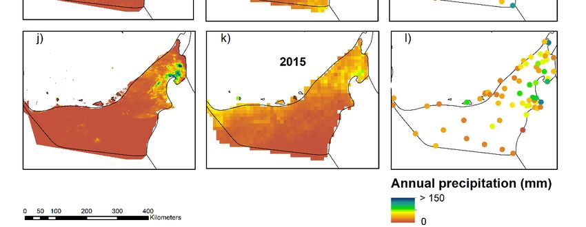
Remote Sens. 2020, 12, 1342                                                                       10 of 28

                                                    Pn
                                                     i=1yest i − yoi
                                         rBIAS =       Pn                                             (8)
                                                        i=1 yoi
                               events detected by both rain gauge and estimate source
                       POD =                                                                          (9)
                                        events detected by rain gauge alone
                                        events dected by estimate source
     FAR =                                                                                           (10)
                total events detected by estimate source including those detected by rain guage
where yest i and yoi are the estimated (model) and observed (gauge) precipitation, respectively, at gauge
i and n is the sample size.
     The model performance is also assessed using the PCC and Nash–Sutcliffe Efficiency (NSE)
coefficients defined by Equations (11) and (12), respectively [91,92]. The PCC records the statistical
association between the model and observational datasets and can range between −1 to 1, where
0 indicates no association and positive/negative values indicate increasing/decreasing relationships
between two variables.
     The NSE records the absolute difference between observed values and corresponding estimates,
normalized by the observational variance to reduce bias. It ranges between −∞ and 1, where values
closer to 1 indicate model accuracy. A threshold value of 0.5 is generally used to imply an adequate
model performance [93,94].
                                            Pn
                                               yo i − yo yest i − yest
                                              i=1
                               PCC = q               2 P               2                          (11)
                                      Pn                  n
                                       i=1 yo i − yo × i=1 yest i − yest

                                                    Pn           2
                                                    yo i − yest i
                                                     i=1
                                       NSE = 1 − P            2                                    (12)
                                                  n
                                                     y
                                                  i=1 oi  − yo

4. Results

4.1. Inter-Comparison of Spatial Distributions
     First, the individual performance of the daily GPM and radar estimates is evaluated against the
overland rain gauge network. Figure 3 shows the spatial distribution of annual rainfall amounts
accumulated from the daily values of the radar, GPM, and rain gauge data. Annual accumulations are
derived for each of the four years (2015–2018) and gridded at their native resolutions. The gauge records
indicate that most of the country’s rainfall events occur around Al Ain and the northeastern highlands,
with 2017 being the wettest (max. observed >300 mm) and 2015 being the driest (max. observed
121 mm). Relatively low rainfall amounts (
RemoteSens.
Remote Sens.2020,
2020,12,
12,1342
x FOR PEER REVIEW 11 of 28
11 of 28
Figure3.3. Spatial
Figure Spatial distribution
distribution of
of daily
daily accumulated
accumulated annual
annual rainfall
rainfall for
for11January
January2015
2015to to31
31December
December
2018
2018(bottom-top)
(bottom-top)from thethe
from radar (a,d,g,j;
radar 0.5 km),
(a,d,g,j; 0.5 GPM
km), (b,e,h,k; 0.1◦ ), and
GPM (b,e,h,k; gauge
0.1°), and(c,f,i,l;
gauge point) datasets.
(c,f,i,l; point)
datasets.
The GPM estimates exhibit a similar spatial organization to the gauge records, with the exception
of 2017
The(Figure 3e) whereexhibit
GPM estimates the highest precipitation
a similar amounts (196
spatial organization mm)
to the are retrieved
gauge overthe
records, with theexception
western
coastline. The GPM product captures most events in the northeastern highlands but
of 2017 (Figure 3e) where the highest precipitation amounts (196 mm) are retrieved over the western with consistent
underestimations
coastline. The GPM compared
producttocaptures
the gauge records,
most eventswhich
in theisnortheastern
mainly attributed to thebut
highlands difference in scale
with consistent
and
underestimations compared to the gauge records, which is mainly attributed to the difference inGPM
missing the short and small-scale local (orographic) convective events. More importantly, the scale
product severely
and missing the underestimates rainfall
short and small-scale around
local Al Ain each
(orographic) year. This
convective is more
events. Moreclearly depictedthe
importantly, in
the
GPM seasonal
productaccumulations shown in Figure
severely underestimates rainfall4,around
whereAl inland gauges
Ain each year.around
This is Al
moreAin record
clearly heavy
depicted
winter precipitation
in the seasonal events (Figure
accumulations shown4f), which are 4,
in Figure missed
whereininland
the GPM product
gauges (Figure
around 4e). record
Al Ain On the heavy
other
hand,
winterlarge overestimations
precipitation events (over
(Figure1004f),
mm) fromare
which GPM are shown
missed in the over
GPMthe coastal(Figure
product areas, particularly
4e). On the
other hand, large overestimations (over 100 mm) from GPM are shown over the coastal areas,Remote Sens. 2020, 12, 1342 12 of 28
Remote Sens. 2020, 12, x FOR PEER REVIEW 12 of 28
during 2016 and
particularly 2017.
during Theand
2016 coastal contamination
2017. The coastal in the GPM product
contamination is GPM
in the pronounced during
product the winter
is pronounced
seasons (Figure 4e) but absent during the summer seasons (Figure 4b).
during the winter seasons (Figure 4e) but absent during the summer seasons (Figure 4b).
Figure 4.
4. Spatial
Spatialdistribution
distribution of
ofaccumulated
accumulated seasonal
seasonal rainfall
rainfall (2015–2018)
(2015–2018) from radar (a,d), GPM
GPM (b,e),
(b,e),
and gauge datasets (c,f) during summer (JJAS) and winter (DJFM) periods.
The radar-based
radar-based precipitation
precipitation pattern
pattern agrees
agrees with
with the
the observed
observed records
records in terms of the spatial
organization, with
organization, with higher
higher amounts
amounts localized
localized in
in the northeastern
northeastern highlands
highlands and
and Al Ain, and lower
amounts to the west. Due
amounts Due toto their
their higher
higher spatial
spatial resolution
resolution (0.5 km), the radar estimates match the
spatial pattern of observed gauge rainfall more closely than the GPM retrievals (10 km). Contrary to
overestimation in
GPM, overestimation in the
the radar
radar product
product is pronounced
pronounced in the summer accumulations
accumulations (Figure
(Figure 4a)
4a)
compared to the gauge amounts (Figure 4c).
attributes
The results thus far suggest the importance of accounting for elevation and land cover attributes
discrepancies between
to address the discrepancies between the
the satellite,
satellite, radar,
radar, and gauge-based
gauge-based precipitation
precipitation estimates.
estimates.
The impact of elevation on the performance of the two precipitation estimates is discussed in the
following subsection.
4.2. Effect
4.2. Effect of
of Topography
Topography on
on Precipitation
Precipitation Estimates
Estimates
The PCC
The PCC value
valueatateach
eachofofthe
the6565gauges
gauges is computed
is computed between the the
between daily gauge
daily observations
gauge and each
observations and
of the corresponding GPM and radar estimates. Figure 5a,b show boxplots of the
each of the corresponding GPM and radar estimates. Figure 5a,b show boxplots of the obtained PCC obtained PCC values
and their
values andvariation as a function
their variation of gauge elevation
as a function of gauge for the GPM
elevation forand
the the
GPM radarandproducts,
the radarrespectively.
products,
The GPM-derived
respectively. PCCs varied from
The GPM-derived PCCs0.21 to 0.76
varied fromwith a median
0.21 valuea of
to 0.76 with 0.53, whereas
median value ofthose
0.53, obtained
whereas
those obtained from the radar estimates showed a larger variance from 0.03 to 0.82, but with of
from the radar estimates showed a larger variance from 0.03 to 0.82, but with a comparable median a
0.48. The larger
comparable interquartile
median of 0.48. range observed
The larger in the radar
interquartile dataobserved
range dictates the
in larger variation
the radar observedthe
data dictates in
the PCCs
larger at lower
variation elevations
observed compared
in the PCCs atto GPM.
lower elevations compared to GPM.Remote Sens. 2020, 12, 1342 13 of 28
Remote Sens. 2020, 12, x FOR PEER REVIEW 13 of 28
Figure 5.
Figure Scatterplotsof
5. Scatterplots ofrecorded
recorded PCC
PCC values
values between
between rain
rain gauge
gauge observations
observations and
and (a)
(a) GPM,
GPM, (b)
(b) radar
radar
precipitation, (c)
precipitation, (c) SMAP
SMAP soil
soil moisture
moisture estimates
estimates versus
versus terrain
terrain elevation.
elevation. Fitted
Fitted power
power law
law curves
curves are
are
displayed for
displayed for each
each scatterplot.
scatterplot.
The power
The power law law relation
relationprovided
providedthe thebest
bestfitfittotothe PCC-elevation
the PCC-elevation dependency
dependency andand
areare
shownshown for
each case. Figure 5a indicates better agreement for GPM estimates at
for each case. Figure 5a indicates better agreement for GPM estimates at higher elevations. higher elevations. Conversely,
Figure 5b shows
Conversely, Figurea 5b
degradation in the radarinperformance
shows a degradation with increasing
the radar performance elevation elevation
with increasing as a result asof a
orography and mountain blockage. This is in line with the annual-scale results
result of orography and mountain blockage. This is in line with the annual-scale results (Figure 3) (Figure 3) with the
northeastern
with highlands
the northeastern associated
highlands with higher
associated withrainfall
higheramounts.
rainfall amounts.
Figure 5c shows the boxplot of the SMAP-derived
Figure 5c shows the boxplot of the SMAP-derived soil moisture soil moisture estimates
estimates at at each
each gauge
gauge location
location
along with
along with the
the PCC-elevation
PCC-elevation scatter
scatter plot.
plot. Correlations
Correlations with with observed
observed rainfall
rainfall record
record anan interquartile
interquartile
range of 0.38 to 0.58 with upper and lower bounds of 0.78 and 0.13, respectively.
range of 0.38 to 0.58 with upper and lower bounds of 0.78 and 0.13, respectively. However, the However, the fitted
fitted
(R2 =
power law
law curve
curve shows
shows aa statistically
statistically insignificant
insignificant decreasing 2
power decreasing relationship
relationship(R 0.24). To
= 0.24). To further
further illicit
illicit
the spatial dependencies of the SMAP-rainfall agreement, Figure 6 shows
the spatial dependencies of the SMAP-rainfall agreement, Figure 6 shows the spatial distribution ofthe spatial distribution of
the PCC recorded at each rain gauge. The subplot (upper-left corner) displays
the PCC recorded at each rain gauge. The subplot (upper-left corner) displays the time series of the the time series of the
retrieved soil
retrieved soilmoisture
moistureand andgauge
gauge rainfall from
rainfall 31 March
from 31 March2015 2015
to 1 January 2019 at2019
to 1 January an arbitrary training
at an arbitrary
gauge. Large co-occurring peaks are observed for five days during the
training gauge. Large co-occurring peaks are observed for five days during the winter periods winter periods (03/01/2016;
10/03/16; 25/01/2017; 3 /cm3 at daily
(03/01/2016; 10/03/16;21/03/2017;
25/01/2017; 17/12/2017),
21/03/2017; with soil moisture
17/12/2017), withvalues reaching values
soil moisture 0.23 cmreaching 0.23
observed
cm 3/cm3 at rainfall amounts over
daily observed 10 mm.
rainfall Less over
amounts pronounced
10 mm.coincident peaks are
Less pronounced seen during
coincident the are
peaks summer
seen
periodsthe
during as asummer
result of periods
light summertime
as a resultprecipitation
of light summertimeassociatedprecipitation
with the sea associated
breeze overwith the western
the sea
region. Better agreement (PCC > 0.4) is observed for low terrain, while less agreement
breeze over the western region. Better agreement (PCC > 0.4) is observed for low terrain, while less (PCC < 0.4) can
be seen over the northeastern highlands.
agreement (PCC < 0.4) can be seen over the northeastern highlands.Remote Sens. 2020, 12, 1342 14 of 28
Remote Sens. 2020, 12, x FOR PEER REVIEW 14 of 28
Figure 6. Spatial
Spatial distribution
distribution of
of PCC
PCC values
values recorded
recorded between
between SMAP
SMAP soil
soil moisture
moisture and
and gauge
gauge rainfall.
rainfall.
Subplot shows the time series of daily SMAP soil moisture and gauge rainfall from 31 March 2015 to
arbitrary training
1 January 2019 at an arbitrary training gauge.
gauge.
The results
resultsindicate the complementary
indicate the complementary performance of the satellite
performance of theand radar-based
satellite and precipitation
radar-based
datasets, withdatasets,
precipitation GPM recommended for the northeastern
with GPM recommended highlands and
for the northeastern radar estimates
highlands and radarfor inland
estimates
and coastal areas, which justifies blending them into one model framework.
for inland and coastal areas, which justifies blending them into one model framework. SMAP soilSMAP soil moisture
estimates record statistically
moisture estimates significantsignificant
record statistically correlations (PCC > 0.5)
correlations with>observed
(PCC 0.5) withrainfall
observedat more than
rainfall at
70%
moreofthan
the gauges,
70% ofshowing that the
the gauges, daily overpasses
showing that the daily(6 am/pm LST) of(6SMAP
overpasses am/pm soilLST)
moisture
of SMAPretrievals
soil
preserve
moisturesurface signature
retrievals preserveofsurface
observed rainfall of
signature events. Thisrainfall
observed is particularly
events. true
This for the inland and
is particularly truelow
for
topography
the inland andareas,
lowwhereas less areas,
topography agreement is observed
whereas in the northern
less agreement is observedhighlands. Nevertheless,
in the northern the
highlands.
recorded agreement
Nevertheless, corroborates
the recorded the use
agreement of the SMAP
corroborates soil of
the use moisture
the SMAP estimates as proxies
soil moisture for daily
estimates as
observed rainfall
proxies for events. rainfall events.
daily observed
4.3. Evaluation of
4.3. Evaluation of Model
Model Performances
Performances
In this section,
In this section, the
the results
results of the fully
of the fully trained
trained GWR
GWR and
and ANN
ANN models
models areare presented. For the
presented. For the same
same
arbitrary
arbitrary training
traininggauge
gaugeused
usedininthe
theprevious
previous section, Figure
section, Figure 7 shows
7 showsthethe
time series
time of daily
series SMAP
of daily SMAPsoil
moisture and rainfall records from the gauges and GPM product, in addition to
soil moisture and rainfall records from the gauges and GPM product, in addition to the corrected the corrected rainfall
estimates from the ANN
rainfall estimates from and
the GWRANN models.
and GWR The GPM product
models. The shows
GPM consistent
product showsunderestimation
consistent
(rBIAS = −24.4%) of observed gauge rainfall, except for large overestimations
underestimation (rBIAS = −24.4%) of observed gauge rainfall, except for large overestimations for three eventsforin
the last quarter of the study period. This is in line with the previous work reporting
three events in the last quarter of the study period. This is in line with the previous work reporting the biases in
GPM estimates
the biases over the
in GPM UAE, attributed
estimates over theto UAE,
ice-scattering microwave
attributed retrieval deficiencies
to ice-scattering microwave over desert
retrieval
land cover [5] and difference in spatial scales [95]. Both models significantly reduce
deficiencies over desert land cover [5] and difference in spatial scales [97]. Both models significantly the bias of the
uncorrected GPM product compared to the rain gauge record. The GWR model
reduce the bias of the uncorrected GPM product compared to the rain gauge record. The GWR model reduced the bias to
−14.6%,
reduced while
the biasthetoANN recorded
−14.6%, while athemore
ANN significant
recordedreduction to 0.7%. reduction to 0.7%.
a more significantRemote Sens. 2020, 12, 1342 15 of 28
Remote Sens. 2020, 12, x FOR PEER REVIEW 15 of 28
Figure
Figure 7. Time
Time series
seriesofofdaily
daily SMAP
SMAP soilsoil moisture
moisture retrievals
retrievals versus
versus rainfall
rainfall records
records from
from (a) rain(a) rain
gauges
gauges
and (b)and
GPM (b)and
GPM and corrected
corrected estimates
estimates from thefrom the (c)and
(c) ANN ANN(d) and
GWR.(d) GWR.
For aa selected
For selected weather
weather event
event on on 33 January
January 2016,
2016, Figure
Figure 88 depicts
depicts thethe precipitation
precipitation amounts
amounts
(mm/day) retrieved
(mm/day) retrieved by
by radar
radarand
andGPM GPMdata,
data,generated
generatedbybythe ANN
the ANN and
andGWR GWR models,
models, recorded
recorded by the
by
rain gauges, as well as the corresponding soil moisture retrievals from the SMAP
the rain gauges, as well as the corresponding soil moisture retrievals from the SMAP product. The product. The rain
gauges
rain recordrecord
gauges between 30 and 30
between 50 mm/day with the event
and 50 mm/day with predominantly impacting the
the event predominantly northeastern
impacting the
UAE, while lighter
northeastern rainfalllighter
UAE, while between 10 and
rainfall 15 mm/day
between 10 andis recorded
15 mm/day inland near Al Ain
is recorded inlandandnearpartsAlofAin
the
northern coastline.
and parts of the northern coastline.
In line
In line with
with the
the previous
previous results
results from
from thethe SMAP-rain
SMAP-rain gauge gauge comparison
comparison (Figure
(Figure 6), 6), the
the soil
soil
moisture conditions
moisture conditions(Figure
(Figure8f)8f) capture
capture thethe spatial
spatial extent
extent ofof the
the weather
weather event
event observed
observed by by the
the rain
rain
gauge distribution
gauge distribution (Figure
(Figure 8e).
8e). Higher
Higher soil
soil moisture values between 0.2 and 0.3 cm33/cm
moisture values /cm33 exist
exist within
within
areas of
areas of observed rainfall,
rainfall, while
whilelower
lowervalues
values(residual
(residualmoisture
moistureasaslow lowasas0.09 cmcm/cm
0.09 3 3/cm3 )3are recorded in
) are recorded
areas
in areasnotnot
impacted
impactedby by
the the
event. TheThe
event. GPM GPM(Figure 8b) estimates
(Figure capture
8b) estimates the event
capture pattern,
the event with lower
pattern, with
underestimations
lower (5–15 (5–15
underestimations mm) over
mm) the
overnortheastern areasareas
the northeastern and higher underestimations
and higher underestimations (20–25 mm)
(20–25
inland
mm) and around
inland Al Ain.AlMore
and around Ain.importantly, the GPM
More importantly, product
the GPM shows
producterroneous rainfall estimates
shows erroneous rainfall
coincidentcoincident
estimates with residual
withsoil moisture
residual soilvalues
moisture andvalues
null gauge rainfall,
and null gauge which is also
rainfall, evident
which during
is also evidentthe
fourth quarter
during of 2018
the fourth in Figure
quarter of 20187b.in Figure 7b.Remote Sens. 2020, 12, 1342 16 of 28
Remote Sens. 2020, 12, x FOR PEER REVIEW 16 of 28
Figure 8.
Figure 8. Precipitation
Precipitation amounts
amounts (mm/day) on 33 January
(mm/day) on January 2016
2016 retrieved
retrieved byby (a)
(a) radar
radar and
and (b)
(b) GPM
GPM data,
data,
inferred by the (c) ANN and (d) GWR models, and observed at (e) rain gauges. Coincident
inferred by the (c) ANN and (d) GWR models, and observed at (e) rain gauges. Coincident SMAP SMAP soil
soil
retrievals are
moisture retrievals are also
also shown
shown (f).
(f).
Figure 8a shows
8Error! the highest
Reference radarnot
source estimates
found.acollocated
shows thewith the highest
highest observed
radar estimates gauge values,
collocated with
but with overestimations
the highest observed gauge of up to 25but
values, mmwith
inland and around Al
overestimations ofAin.
up toFurthermore,
25 mm inland theand
radar pattern
around Al
shows clear gaps from
Ain. Furthermore, themountain blockage
radar pattern showsoverclear
the farthest
gaps fromnortheastern
mountainarea bordering
blockage overOman, where
the farthest
the maximumarea
northeastern observed rain Oman,
bordering gauge values
wherearethelocated.
maximum observed rain gauge values are located.
Both the
Both theANN
ANN andand
GWR GWR precipitation
precipitation outputsoutputs
in Figurein8c,d,
Figure 8c,d, respectively,
respectively, exhibit an
exhibit an intermediary
intermediary
pattern betweenpattern between
the radar andthe
GPMradar and GPM representations.
representations. Both modelsBoth models
increase theincrease the event
event extent and
extent andrainfall
resulting resulting rainfall
over over the northeastern
the northeastern domain and domain and more
more closely closely
match the match
gauge the
andgauge and soil
soil moisture
moisture distributions. The major differences between the ANN and GWR results exist over the
poorly gauged western region. Compared to the GWR pattern, the ANN pattern more closely
matches the soil moisture fields from SMAP. This suggests the ANN model’s capability to integrateYou can also read