Daily evaluation of 26 precipitation datasets using Stage-IV gauge-radar data for the CONUS - HESS
←
→
Page content transcription
If your browser does not render page correctly, please read the page content below
Hydrol. Earth Syst. Sci., 23, 207–224, 2019
https://doi.org/10.5194/hess-23-207-2019
© Author(s) 2019. This work is distributed under
the Creative Commons Attribution 4.0 License.

Daily evaluation of 26 precipitation datasets using Stage-IV
gauge-radar data for the CONUS
Hylke E. Beck1 , Ming Pan1 , Tirthankar Roy1 , Graham P. Weedon2 , Florian Pappenberger3 , Albert I. J. M. van Dijk4 ,
George J. Huffman5 , Robert F. Adler6 , and Eric F. Wood1
1 Department  of Civil and Environmental Engineering, Princeton University, Princeton, New Jersey, USA
2 Met Office, JCHMR, Maclean Building, Benson Lane, Crowmarsh Gifford, Oxfordshire, UK
3 European Centre for Medium-Range Weather Forecasts (ECMWF), Reading, UK
4 Fenner School for Environment and Society, Australian National University, Canberra, Australia
5 NASA Goddard Space Flight Center (GSFC), Greenbelt, Maryland, USA
6 University of Maryland, Earth System Science Interdisciplinary Center, College Park, Maryland, USA

Correspondence: Hylke E. Beck (hylke.beck@gmail.com)

Received: 9 September 2018 – Discussion started: 27 September 2018
Revised: 26 December 2018 – Accepted: 3 January 2019 – Published: 16 January 2019

Abstract. New precipitation (P ) datasets are released regu-    stantially better than TMPA-3B42RT V7, attributable to the
larly, following innovations in weather forecasting models,     many improvements implemented in the IMERG satellite P
satellite retrieval methods, and multi-source merging tech-     retrieval algorithm. IMERGHH V05 outperformed ERA5-
niques. Using the conterminous US as a case study, we eval-     HRES in regions dominated by convective storms, while the
uated the performance of 26 gridded (sub-)daily P datasets      opposite was observed in regions of complex terrain. The
to obtain insight into the merit of these innovations. The      ERA5-EDA ensemble average exhibited higher correlations
evaluation was performed at a daily timescale for the period    than the ERA5-HRES deterministic run, highlighting the
2008–2017 using the Kling–Gupta efficiency (KGE), a per-        value of ensemble modeling. The WRF regional convection-
formance metric combining correlation, bias, and variability.   permitting climate model showed considerably more accu-
As a reference, we used the high-resolution (4 km) Stage-IV     rate P totals over the mountainous west and performed best
gauge-radar P dataset. Among the three KGE components,          among the uncorrected datasets in terms of variability, sug-
the P datasets performed worst overall in terms of correla-     gesting there is merit in using high-resolution models to ob-
tion (related to event identification). In terms of improving   tain climatological P statistics. Our findings provide some
KGE scores for these datasets, improved P totals (affecting     guidance to choose the most suitable P dataset for a particu-
the bias score) and improved distribution of P intensity (af-   lar application.
fecting the variability score) are of secondary importance.
Among the 11 gauge-corrected P datasets, the best overall
performance was obtained by MSWEP V2.2, underscoring
                                                                1   Introduction
the importance of applying daily gauge corrections and ac-
counting for gauge reporting times. Several uncorrected P       Knowledge about the spatio-temporal distribution of pre-
datasets outperformed gauge-corrected ones. Among the 15        cipitation (P ) is important for a multitude of scientific and
uncorrected P datasets, the best performance was obtained       operational applications, including flood forecasting, agri-
by the ERA5-HRES fourth-generation reanalysis, reflecting       cultural monitoring, and disease tracking (Tapiador et al.,
the significant advances in earth system modeling during the    2012; Kucera et al., 2013; Kirschbaum et al., 2017). How-
last decade. The (re)analyses generally performed better in     ever, P is highly variable in space and time and there-
winter than in summer, while the opposite was the case for      fore extremely challenging to estimate, especially in topo-
the satellite-based datasets. IMERGHH V05 performed sub-        graphically complex, convection-dominated, and snowfall-

Published by Copernicus Publications on behalf of the European Geosciences Union.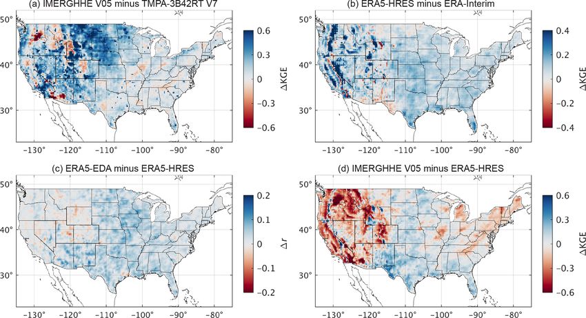
208                                          H. E. Beck et al.: Daily evaluation of 26 precipitation datasets for the CONUS

dominated regions (Stephens et al., 2010; Tian and Peters-         formance metric, we adopt the widely used Kling–Gupta
Lidard, 2010; Herold et al., 2016; Prein and Gobiet, 2017).        efficiency (KGE; Gupta et al., 2009; Kling et al., 2012).
In the past decades, numerous gridded P datasets have been         We shed light on the strengths and weaknesses of different
developed, differing in terms of design objective, spatio-         P datasets and on the merit of different technological and
temporal resolution and coverage, data sources, algorithm,         methodological innovations by addressing 10 pertinent
and latency (see Tables 1 and 2 for an overview of quasi and       questions.
fully global datasets).
   A large number of regional-scale studies have evaluated             1. What is the most important factor determining a high
gridded P datasets to obtain insight into the merit of differ-            KGE score?
ent methods and innovations (see reviews by Gebremichael,
                                                                       2. How do the uncorrected P datasets perform?
2010, Maggioni et al., 2016, and Sun et al., 2018). However,
many of these studies (i) used only a subset of the avail-             3. How do the gauge-based P datasets perform?
able P datasets, and omitted (re)analyses, which have higher
skill in cold periods and regions (Huffman et al., 1995; Ebert         4. How do the P datasets perform in summer versus win-
et al., 2007; Beck et al., 2017c); (ii) focused on a small (sub-          ter?
continental) region, limiting the generalizability of the find-
                                                                       5. What is the impact of gauge corrections?
ings; (iii) considered a small number (< 50) of rain gauges or
streamflow gauging stations for the evaluation, limiting the           6. What is the improvement of IMERG over TMPA?
validity of the findings; (iv) used gauge observations already
incorporated into the datasets as a reference without explic-          7. What is the improvement of ERA5 over ERA-Interim?
itly mentioning this, potentially leading to a biased evalua-
                                                                       8. How does the ERA5-EDA ensemble average compare
tion; and (v) failed to account for gauge reporting times, pos-
                                                                          to the ERA5-HRES deterministic run?
sibly resulting in spurious temporal mismatches between the
datasets and the gauge observations.                                   9. How do IMERG and ERA5 compare?
   In an effort to obtain more generally valid conclusions,
we recently evaluated 22 (sub-)daily gridded P datasets us-        10. How well does a regional convection-permitting climate
ing gauge observations (∼ 75 000 stations) and hydrological            model perform?
modeling (∼ 9000 catchments) globally (Beck et al., 2017c).
Other noteworthy large-scale assessments include Tian and
Peters-Lidard (2010), who quantified the uncertainty in P          2     Data and methods
estimates by comparing six satellite-based datasets, Massari
et al. (2017), who evaluated five P datasets using triple collo-   2.1    P datasets
cation at the daily timescale without the use of ground obser-
vations, and Sun et al. (2018), who compared 19 P datasets         We evaluated the performance of 26 gridded (sub-)daily P
at daily to annual timescales. These comprehensive studies         datasets (Tables 1 and 2). All datasets are either fully or
highlighted (among other things) (i) substantial differences       near global, with the exception of WRF, which is limited
among P datasets and thus the importance of dataset choice;        to the CONUS. The datasets are classified as either un-
(ii) the complementary strengths of satellite and (re)analysis     corrected, which implies that temporal variations depend
P datasets; (iii) the value of merging P estimates from dis-       entirely on satellite and/or (re)analysis data, or corrected,
parate sources; (iv) the effectiveness of daily (as opposed to     which implies that temporal variations depend to some de-
monthly) gauge corrections; and (v) the widespread underes-        gree on gauge observations. We included seven datasets ex-
timation of P in mountainous regions.                              clusively based on satellite data (CMORPH V1.0, GSMaP-
   Here, we evaluate an even larger selection of (sub-)daily       Std V6, IMERGHHE V05, PERSIANN, PERSIANN-CCS,
(quasi-)global P datasets for the conterminous US                  SM2RAIN-CCI V2, and TMPA-3B42RT V7), six fully based
(CONUS), including some promising recently released                on (re)analyses (ERA-Interim, ERA5-HRES, ERA5-EDA,
datasets: ERA5 (the successor to ERA-Interim; Hersbach             GDAS-Anl, JRA-55, and NCEP-CFSR, although ERA5 as-
et al., 2018), IMERG (the successor to TMPA; Huffman               similates radar and gauge data over the CONUS), one incor-
et al., 2014, 2018), and MERRA-2 (one of the few reanalysis        porating both satellite and (re)analysis data (CHIRP V2.0),
P datasets incorporating daily gauge observations; Gelaro          and one based on a regional convection-permitting climate
et al., 2017; Reichle et al., 2017). In addition, we evaluate      model (WRF).
the performance of a regional convection-permitting climate           Among the gauge-based P datasets, six combined gauge
model (WRF; Liu et al., 2017). As a reference, we use the          and satellite data (CMORPH-CRT V1.0, GPCP-1DD V1.2,
high-resolution, radar-based, gauge-adjusted Stage-IV P            GSMaP-Std Gauge V7, IMERGDF V05, PERSIANN-
dataset (Lin and Mitchell, 2005) produced by the National          CDR V1R1, and TMPA-3B42 V7), one combined gauge
Centers for Environmental Prediction (NCEP). As a per-             and reanalysis data (WFDEI-GPCC), three combined gauge,

Hydrol. Earth Syst. Sci., 23, 207–224, 2019                                        www.hydrol-earth-syst-sci.net/23/207/2019/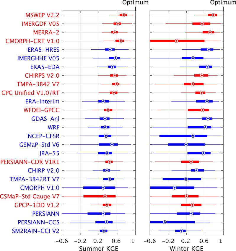
H. E. Beck et al.: Daily evaluation of 26 precipitation datasets for the CONUS                                                                                                                                                 209

Table 1. Overview of the 15 uncorrected (quasi-)global (sub-)daily gridded P datasets evaluated in this study. The 11 gauge-corrected
datasets are listed in Table 2. Abbreviations in the data source(s) column defined as S, satellite; R, reanalysis; A, analysis; and M, regional
climate model. The abbreviation NRT in the temporal coverage column stands for near real time. In the spatial coverage column, “Global”
means fully global coverage including oceans, while “Land” means that the coverage is limited to the terrestrial land surface.

 Name                          Details                                                            Data            Spatial           Spatial                Temporal         Temporal               Reference or website
                                                                                                  source(s)       resolution        coverage               resolution       coverage
 CHIRP V2.01                   Climate Hazards group InfraRed Precipitation                       S, R, A         0.05◦             Land, 50◦ N/S          Daily            1981–NRT3              Funk et al. (2015a)
                               (CHIRP) V2.0
 CMORPH V1.0                   CPC MORPHing technique (CMORPH) V1.0                               S               0.07◦             60◦ N/S                30 min           1998–NRT2              Joyce et al. (2004),
                                                                                                                                                                                                   Xie et al. (2017)
 ERA-Interim                   European Centre for Medium-range Weather                           R               ∼ 0.75◦           Global                 3-hourly         1979–NRT4              Dee et al. (2011)
                               Forecasts ReAnalysis Interim (ERA-Interim)
 ERA5-HRES5                    European Centre for Medium-range Weather                           R               ∼ 0.28◦           Global                 Hourly           2008–NRT3, 6           Hersbach et al. (2018)
                               Forecasts ReAnalysis 5 (ERA5) High RESolu-
                               tion (HRES)
 ERA5-EDA5                     European Centre for Medium-range Weather                           R               ∼ 0.56◦           Global                 Hourly           2008–NRT3, 6           Hersbach et al. (2018)
                               Forecasts ReAnalysis 5 (ERA5) Ensemble Data
                               Assimilation (EDA) ensemble mean
 GDAS-Anl                      National Centers for Environmental Predic-                         A               ∼ 0.25◦           Global                 3-hourly         2015–NRT2              http://www.emc.ncep.
                               tion (NCEP) Global Data Assimilation System                                                                                                                         noaa.gov/gmb/gdas/
                               (GDAS) Analysis (Anl)                                                                                                                                               (last access: August
                                                                                                                                                                                                   2018)
 GSMaP-Std V6                  Global Satellite Mapping of Precipitation                          S               0.1◦              60◦ N/S                Hourly           2000–NRT2              Ushio et al. (2009)
                               (GSMaP) Moving Vector with Kalman (MVK)
                               Standard V6
 IMERGHHE V05                  Integrated Multi-satellitE Retrievals for GPM                      S               0.1◦              60◦ N/S                30 min           2014–NRT2, 7           Huffman et al. (2014,
                               (IMERG) early run V05                                                                                                                                               2018)
 JRA-55                        Japanese 55 year ReAnalysis (JRA-55)                               R               ∼ 0.56◦           Global                 3-hourly         1959–NRT3              Kobayashi et al. (2015)
 NCEP-CFSR                     National Centers for Environmental Prediction                      R               ∼ 0.31◦           Global                 Hourly           1979–2010              Saha et al. (2010)
                               (NCEP) Climate Forecast System Reanalysis
                               (CFSR)
 PERSIANN                      Precipitation Estimation from Remotely Sensed                      S               0.25◦             60◦ N/S                Hourly           2000–NRT2              Sorooshian et al. (2000)
                               Information using Artificial Neural Networks
                               (PERSIANN)
 PERSIANN-CCS                  Precipitation Estimation from Remotely Sensed                      S               0.04◦             60◦ N/S                Hourly           2003–NRT2              Hong et al. (2004)
                               Information using Artificial Neural Networks
                               (PERSIANN) Cloud Classification System
                               (CCS)
 SM2RAIN-CCI V2                Rainfall inferred from European Space                              S               0.25◦             Land                   Daily            1998–2015              Ciabatta et al. (2018)
                               Agency’s (ESA) Climate Change Initiative
                               (CCI) satellite near-surface soil moisture V2
 TMPA-3B42RT V7                TRMM Multi-satellite Precipitation Analysis                        S               0.25◦             50◦ N/S                3-hourly         2000–NRT2              Huffman et al. (2007)
                               (TMPA) 3B42RT V7
 WRF8                          Weather Research and Forecasting (WRF)                             M               4 km              CONUS                  Hourly           2000–2013              Liu et al. (2017)
1 The daily variability is based on satellite and reanalysis data. However, the monthly climatology has been corrected using a gauge-based dataset (Funk et al., 2015b). 2 Available until the present with a delay of several hours.
3 Available until the present with a delay of several days. 4 Available until the present with a delay of several months. 5 Rain gauge and ground radar observations were assimilated from 17 July 2009 onwards (Lopez, 2011,
2013). 6 1950–NRT once production has been completed. 7 2000–NRT for the next version. 8 The only dataset included in the evaluation with continental coverage instead of (quasi-)global coverage.

satellite, and (re)analysis data (CHIRPS V2.0, MERRA-2,                                                                with spatial resolutions > 0.1◦ were resampled to 0.1◦ using
and MSWEP V2.2), while one was fully based on gauge                                                                    bilinear interpolation.
observations (CPC Unified V1.0/RT). For transparency and
reproducibility, we report dataset version numbers through-                                                            2.2       Stage-IV gauge-radar data
out the study for the datasets for which this information
was provided. For the P datasets with a sub-daily tempo-                                                               As a reference, we used the NCEP Stage-IV dataset, which
ral resolution, we calculated daily accumulations for 00:00–                                                           has a 4 km spatial and hourly temporal resolution and cov-
23:59 UTC. P datasets with spatial resolutions < 0.1◦ were                                                             ers the period 2002 until the present, and merges data from
resampled to 0.1◦ using bilinear averaging, whereas those                                                              140 radars and ∼ 5500 gauges over the CONUS (Lin and
                                                                                                                       Mitchell, 2005). Stage-IV provides highly accurate P esti-
                                                                                                                       mates and has therefore been widely used as a reference for

www.hydrol-earth-syst-sci.net/23/207/2019/                                                                                                         Hydrol. Earth Syst. Sci., 23, 207–224, 2019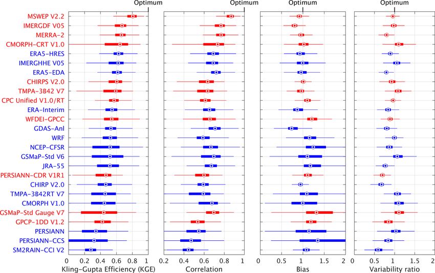
210                                                             H. E. Beck et al.: Daily evaluation of 26 precipitation datasets for the CONUS

Table 2. Overview of the 11 gauge-corrected (quasi-)global (sub-)daily gridded P datasets evaluated in this study. The 15 uncorrected
datasets are listed in Table 1. Abbreviations in the data source(s) column defined as G, gauge; S, satellite; R, reanalysis; and A, analysis. The
abbreviation NRT in the temporal coverage column stands for near real time. In the spatial coverage column, “global” indicates fully global
coverage including ocean areas, while “land” indicates that the coverage is limited to the terrestrial surface.

  Name                 Details                                             Data           Spatial        Spatial            Temporal       Temporal           Reference or website
                                                                           source(s)      resolution     coverage           resolution     coverage
  CHIRPS V2.0          Climate Hazards group InfraRed Precipita-           G, S, R, A     0.05◦          Land, 50◦ N/S      Daily          1981–NRT2          Funk et al. (2015a)
                       tion with Stations (CHIRPS) V2.0
  CMORPH-              CPC MORPHing technique (CMORPH)                     G, S           0.07◦          60◦ N/S            30 min         1998–2015          Joyce et al. (2004),
  CRT V1.0             bias corrected (CRT) V1.0                                                                                                              Xie et al. (2017)
  CPC Unified          Climate Prediction Center (CPC) Unified             G              0.5◦           Land               Daily          1979–NRT2          Xie et al. (2007),
  V1.0/RT              V1.0 and RT                                                                                                                            Chen et al. (2008)
  GPCP-1DD             Global Precipitation Climatology Project            G, S           1◦             Global             Daily          1996–2015          Huffman et al. (2001)
  V1.2                 (GPCP) 1-Degree Daily (1DD) Combina-
                       tion V1.2
  GSMaP-Std            Global Satellite Mapping of Precipitation           G, S           0.1◦           60◦ N/S            Hourly         2000–NRT1          Ushio et al. (2009)
  Gauge V7             (GSMaP) Moving Vector with Kalman
                       (MVK) Standard gauge-corrected V7
  IMERGDF V05          Integrated Multi-satellitE Retrievals for           G, S           0.1◦           60◦ N/S            30 min         2014–NRT3, 4       Huffman et al. (2014,
                       GPM (IMERG) final run V05                                                                                                              2018)
  MERRA-2              Modern-Era Retrospective Analysis for Re-           G, S, R        ∼ 0.5◦         Global             Hourly         1980–NRT3          Gelaro et al. (2017),
                       search and Applications 2                                                                                                              Reichle et al. (2017)
  MSWEP V2.2           Multi-Source Weighted-Ensemble Precipi-             G, S, R, A     0.1◦           Global             3-hourly       1979–NRT1          Beck et al. (2017b,
                       tation (MSWEP) V2.2                                                                                                                    2019)
  PERSIANN-            Precipitation Estimation from Remotely              G, S           0.25◦          60◦ N/S            Daily          1983–2016          Ashouri et al. (2015)
  CDR V1R1             Sensed Information using Artificial Neu-
                       ral Networks (PERSIANN) Climate Data
                       Record (CDR) V1R1
  TMPA-3B42            TRMM Multi-satellite Precipitation Analy-           G, S           0.25◦          50◦ N/S            3-hourly       2000–2017          Huffman et al. (2007)
  V7                   sis (TMPA) 3B42 V7
  WFDEI-GPCC           WATCH Forcing Data ERA-Interim                      G, R           0.5◦           Land               3-hourly       1979–2016          Weedon et al. (2014)
                       (WFDEI) corrected using Global Precipita-
                       tion Climatology Centre (GPCC)
1 Available until the present with a delay of several hours. 2 Available until the present with a delay of several days. 3 Available until the present with a delay of several months.
4 2000–NRT for the next version.

the evaluation of P datasets (e.g., Hong et al., 2006; Habib                                      ing bilinear averaging. The PRISM dataset has been derived
et al., 2009; AghaKouchak et al., 2011, 2012; Nelson et al.,                                      from gauge observations using a sophisticated interpolation
2016; Zhang et al., 2018b). Daily Stage-IV data are available,                                    approach that accounts for topography. It is generally con-
but they represent an accumulation period that is incompat-                                       sidered the most accurate monthly P dataset available for
ible with the datasets we are evaluating (12:00–11:59 UTC                                         the US and has been used as a reference in numerous studies
instead of 00:00–23:59 UTC). We therefore calculated daily                                        (e.g., Mizukami and Smith, 2012; Prat and Nelson, 2015; Liu
accumulations for 00:00–23:59 UTC from 6-hourly Stage-IV                                          et al., 2017). However, the dataset has not been corrected for
accumulations. The Stage-IV dataset was reprojected from                                          wind-induced gauge undercatch and thus may underestimate
its native 4 km polar stereographic projection to a regular ge-                                   P to some degree (Groisman and Legates, 1994; Rasmussen
ographic 0.1◦ grid using bilinear averaging.                                                      et al., 2012).
   The Stage-IV dataset is a mosaic of regional analyses pro-
duced by 12 CONUS River Forecast Centers (RFCs) and is                                            2.3   Evaluation approach
thus subject to the gauge correction and quality control per-
formed at each individual RFC (Westrick et al., 1999; Smal-
                                                                                                  The evaluation was performed at a daily temporal and 0.1◦
ley et al., 2014; Eldardiry et al., 2017). To reduce systematic
                                                                                                  spatial resolution by calculating, for each grid cell, KGE
biases, the Stage-IV dataset was rescaled such that its long-
                                                                                                  scores from daily time series for the 10-year period from
term mean matches that of the PRISM dataset (Daly et al.,
                                                                                                  2008 to 2017. KGE is an objective performance metric com-
2008) for the evaluation period (2008–2017). To this end,
                                                                                                  bining correlation, bias, and variability. It was introduced in
the PRISM dataset was upscaled from ∼ 800 m to 0.1◦ us-
                                                                                                  Gupta et al. (2009) and modified in Kling et al. (2012) and is

Hydrol. Earth Syst. Sci., 23, 207–224, 2019                                                                           www.hydrol-earth-syst-sci.net/23/207/2019/
H. E. Beck et al.: Daily evaluation of 26 precipitation datasets for the CONUS 211
defined as follows: last decade. The third-generation, coarser-resolution reanal-
q yses (ERA-Interim, JRA-55, and NCEP-CFSR) performed
KGE = 1 − (r − 1)2 + (β − 1)2 + (γ − 1)2 , (1) slightly worse overall (median KGE of 0.55, 0.52, and 0.52,
respectively). ERA-Interim performed slightly better than
where the correlation component r is represented by (Pear- other third-generation reanalyses, consistent with earlier
son’s) correlation coefficient, the bias component β by the studies focusing on P (Bromwich et al., 2011; Peña Aran-
ratio of estimated and observed means, and the variability cibia et al., 2013; Palerme et al., 2017; Beck et al., 2017c) and
component γ by the ratio of the estimated and observed co- other atmospheric variables (Bracegirdle and Marshall, 2012;
efficients of variation: Jin-Huan et al., 2014; Zhang et al., 2016). All (re)analyses,
µs σs /µs including the new ERA5-HRES, underestimated the variabil-
β= and γ = , (2) ity (Figs. 2 and S3 in the Supplement), reflecting the ten-
µo σo /µo
dency of (re)analyses to overestimate P frequency (Zolina
where µ and σ are the distribution mean and standard devia- et al., 2004; Sun et al., 2006; Lopez, 2007; Stephens et al.,
tion, respectively, and the subscripts s and o indicate estimate 2010; Skok et al., 2015; Beck et al., 2017c). The addi-
and reference, respectively. KGE, r, β, and γ values all have tional variability underestimation by ERA5-EDA compared
their optimum at unity. to ERA5-HRES probably reflects the variance loss induced
by the averaging.
Among the uncorrected satellite-based P datasets, the
3 Results and discussion new IMERGHHE V05 performed best overall by a sub-
stantial margin (median KGE of 0.62; Figs. 1 and 2), re-
3.1 What is the most important factor determining a
flecting the quality of the new IMERG P retrieval algo-
high KGE score?
rithm (Huffman et al., 2014, 2018). The other passive-
Figure 2 presents box-and-whisker plots of KGE scores for microwave-based datasets (CMORPH V1.0, GSMaP-Std V6,
the 26 P datasets. The mean median KGE score over all and TMPA-3B42RT V7) obtained median KGE scores
datasets is 0.54. The mean median scores for the correlation, ranging from 0.44 to 0.52. CHIRP V2.0, which com-
bias, and variability components of the KGE, expressed as bines infrared- and reanalysis-based estimates, performed
|r − 1|, |β − 1|, and |γ − 1|, are 0.34, 0.18, and 0.16, respec- similarly to some of the passive-microwave datasets (me-
tively (see Eq. 1). The datasets thus performed considerably dian KGE of 0.47). The datasets exclusively based on in-
worse in terms of correlation, which makes sense given that frared data (PERSIANN and PERSIANN-CCS) performed
long-term climatological P statistics are easier to estimate markedly worse (median KGE of 0.34 and 0.32, respec-
than day-to-day P dynamics. Due to the squaring of the three tively), consistent with previous P dataset evaluations (e.g.,
components in the KGE equation (see Eq. 1), the correla- Hirpa et al., 2010; Peña Arancibia et al., 2013; Cattani et al.,
tion values exert the dominant influence on the final KGE 2016; Beck et al., 2017c). This has been attributed to the in-
scores. Indeed, the performance ranking in terms of KGE direct nature of the relationship between cloud-top temper-
corresponds well to the performance ranking in terms of cor- atures and surface rainfall (Adler and Negri, 1988; Vicente
relation (Fig. 2). These results suggest that in order to get an et al., 1998; Scofield and Kuligowski, 2003). The infrared-
improved KGE score, the most important component score based datasets generally exhibited a much larger spatial vari-
to improve is the correlation. This in turn suggests that, for ability in performance for all four metrics (Figs. 1 and S1–
existing daily P datasets, improvements to the timing of P S3).
events at the daily scale (dominating the correlation scores) The (uncorrected) satellite soil moisture-based
are more valuable than improvements to P totals (dominat- SM2RAIN-CCI V2 dataset performed comparatively
ing bias scores) or the intensity distribution (dominating vari- poorly (median KGE of 0.28; Figs. 1 and 2). The dataset
ability scores). strongly underestimated the variability (Fig. S3), due to the
noisiness of satellite soil moisture retrievals and the inability
3.2 How do the uncorrected P datasets perform? of satellite soil moisture-based algorithms to detect rainfall
exceeding the soil water storage capacity (Zhan et al., 2015;
Among the uncorrected P datasets, the (re)analyses per- Wanders et al., 2015; Tarpanelli et al., 2017; Ciabatta et al.,
formed better overall than the satellite-based datasets (Figs. 1 2018). At high latitudes and elevations, the presence of snow
and 2). The best performance was obtained by ECMWF’s and frozen soils may have hampered performance (Brocca
fourth-generation reanalysis ERA5-HRES (median KGE et al., 2014), while in arid regions, irrigation may have been
of 0.63), with NASA’s most recent satellite-based dataset misinterpreted as rainfall (Brocca et al., 2018). In addition,
IMERGHHE V05 and the ensemble average ERA5-EDA approximately 25 % (in the eastern CONUS) to 50 % (over
coming a close equal second (median KGE of 0.62). These the mountainous west) of the daily rainfall values were based
results underscore the substantial advances in earth sys- on temporal interpolation, to fill gaps in the satellite soil
tem modeling and satellite-based P estimation over the moisture data (Dorigo et al., 2017). Despite these limitations,
www.hydrol-earth-syst-sci.net/23/207/2019/ Hydrol. Earth Syst. Sci., 23, 207–224, 2019212 H. E. Beck et al.: Daily evaluation of 26 precipitation datasets for the CONUS
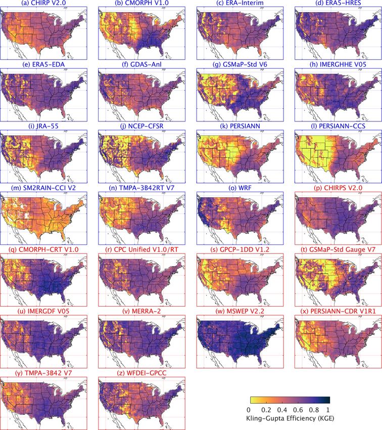
Figure 1. KGE scores for the 26 gridded P datasets using the Stage-IV gauge-radar dataset as a reference. White indicates missing data.
Higher KGE values correspond to better performance. Uncorrected datasets are listed in blue, whereas gauge-corrected datasets are listed
in red. Details on the datasets are provided in Tables 1 and 2. Maps for the correlation, bias, and variability components of the KGE are
presented in the Supplement.
the SM2RAIN datasets may provide new possibilities for All uncorrected P datasets exhibited lower overall perfor-
evaluation (Massari et al., 2017) and correction (Massari mance in the western CONUS (Figs. 1, 2, and S1–S3), in line
et al., 2018) of other P datasets, since they constitute a fully with previous studies (e.g., Gottschalck et al., 2005; Ebert
independent, alternative source of rainfall data. et al., 2007; Tian et al., 2007; AghaKouchak et al., 2012;
Chen et al., 2013; Beck et al., 2017c; Gebregiorgis et al.,
Hydrol. Earth Syst. Sci., 23, 207–224, 2019 www.hydrol-earth-syst-sci.net/23/207/2019/H. E. Beck et al.: Daily evaluation of 26 precipitation datasets for the CONUS 213
Figure 2. Box-and-whisker plots of KGE scores for the 26 gridded P datasets using the Stage-IV gauge-radar dataset as a reference. The
circles represent the median value, the left and right edges of the box represent the 25th and 75th percentile values, respectively, while the
“whiskers” represent the extreme values. The statistics were calculated for each dataset from the distribution of grid-cell KGE values (no
area weighting was performed). The datasets are sorted in ascending order of the median KGE. Uncorrected datasets are indicated in blue,
whereas gauge-corrected datasets are indicated in red. Details on the datasets are provided in Tables 1 and 2.
2018). This is attributable to the more complex topography 3.3 How do the gauge-based P datasets perform?
and greater spatio-temporal heterogeneity of P in the west
(Daly et al., 2008), which affects the quality of both the eval-
Among the gauge-based P datasets, the best overall per-
uated datasets and the reference (Westrick et al., 1999; Smal-
formance was obtained by MSWEP V2.2 (median KGE
ley et al., 2014; Eldardiry et al., 2017). With the exception of
of 0.81), followed at some distance by IMERGDF V05 (me-
CHIRP V2.0 (which has been corrected for systematic biases
dian KGE of 0.67) and MERRA-2 (median KGE of 0.66;
using gauge observations; Funk et al., 2015b) and WRF (the
Figs. 1 and 2). IMERGDF V05 exhibited a small nega-
high-resolution climate simulation; Liu et al., 2017), the (un-
tive bias, while MERRA-2 slightly underestimated the vari-
corrected) datasets exhibited large P biases over the moun-
ability. The good performance obtained by MSWEP V2.2
tainous west (Fig. S2), which is in agreement with earlier
underscores the importance of incorporating daily gauge
studies using other reference datasets (Adam et al., 2006;
data and accounting for reporting times (Beck et al.,
Kauffeldt et al., 2013; Beck et al., 2017a; Beck et al., 2017c)
2019). While CMORPH-CRT V1.0, CPC Unified V1.0/RT,
and reflects the difficulty of retrieving and simulating oro-
GSMaP-Std Gauge V7, and MERRA-2 also incorporate
graphic P (Roe, 2005). We initially expected bias values to
daily gauge data, they did not account for reporting times, re-
be higher than unity since PRISM, the dataset used to correct
sulting in temporal mismatches and hence lower KGE scores
systematic biases in Stage-IV (see Sect. 2.2), lacks explicit
(Fig. 2). Reporting times in the CONUS range from mid-
gauge undercatch corrections (Daly et al., 2008), but this did
night −12 to +9 h UTC for the stations in the comprehen-
not appear to be the case (Figs. 2 and S2).
sive GHCN-D gauge database (Menne et al., 2012; Fig. 2c
in Beck et al., 2019), suggesting that up to half of the daily
P accumulations may be assigned to the wrong day. In ad-
dition, CMORPH-CRT V1.0, GSMaP-Std Gauge V7, and
www.hydrol-earth-syst-sci.net/23/207/2019/ Hydrol. Earth Syst. Sci., 23, 207–224, 2019214 H. E. Beck et al.: Daily evaluation of 26 precipitation datasets for the CONUS
MERRA-2 applied daily gauge corrections using CPC Uni- – The datasets incorporating both satellite and reanal-
fied (Xie et al., 2007; Chen et al., 2008), which has a rel- ysis estimates (CHIRP V2.0, CHIRPS V2.0, and
atively coarse 0.5◦ resolution, whereas MSWEP V2.2 ap- MSWEP V2.2) performed similarly in both seasons,
plied corrections at 0.1◦ resolution based on the five nearest taking advantage of the accuracy of satellite retrievals
gauges for each grid cell (Beck et al., 2019). The good per- in summer and reanalysis outputs in winter (Ebert et al.,
formance of IMERGDF V05 is somewhat surprising, given 2007; Beck et al., 2017b). The fully gauge-based CPC
the use of monthly rather than daily gauge data, and attests Unified V1.0/RT also performed similarly in both sea-
to the quality of the IMERG P retrieval algorithm (Huffman sons.
et al., 2014, 2018).
Similar to the uncorrected datasets, the corrected estimates
3.5 What is the impact of gauge corrections?
consistently performed worse in the west (Figs. 1, 2, and S1–
S3), due not only to the greater spatio-temporal heterogene- Differences in median KGE values between uncorrected and
ity in P (Daly et al., 2008), but also the lower gauge network gauge-corrected versions of P datasets ranged from −0.07
density (Kidd et al., 2017). It should be kept in mind that the (GSMaP-Std Gauge V7) to +0.20 (CMORPH-CRT V1.0;
performance ranking may differ across the globe depending Table 3). GSMaP-Std Gauge V7 shows a large positive bias
on the amount of gauge data ingested and the quality con- in the west (Fig. S2), suggesting that its gauge-correction
trol applied for each dataset. Thus, the results found here for methodology requires re-evaluation. The substantial im-
the CONUS do not necessarily directly generalize to other provements in median KGE for CHIRPS V2.0 (+0.13) and
regions. CMORPH-CRT V1.0 (+0.20) reflect the use of sub-monthly
gauge data (5-day and daily, respectively). Conversely, the
3.4 How do the P datasets perform in summer versus datasets incorporating monthly gauge data (IMERGDF V05
winter? and WFDEI-GPCC) exhibited little to no improvement in
median KGE (+0.05 and −0.01, respectively), suggest-
Figure 3 presents KGE values for summer and winter for the
ing that monthly corrections provide little to no benefit
26 P datasets. The following observations can be made.
at the daily timescale of the present evaluation (Tan and
Santo, 2018). These results, combined with the fact that sev-
– The spread in median KGE values among the datasets
eral uncorrected P datasets outperformed gauge-corrected
is much greater in winter than in summer. In addition,
ones (Fig. 2), suggest that a P dataset labeled as “gauge-
almost all datasets exhibit a greater spatial variability in
corrected” is not necessarily always the better choice.
KGE values in winter, as indicated by the wider boxes
and whiskers. This is probably at least partly attributable 3.6 What is the improvement of IMERG over TMPA?
to the lower quality of the Stage-IV dataset in winter
(Westrick et al., 1999; Smalley et al., 2014; Eldardiry IMERG (Huffman et al., 2014, 2018) is NASA’s latest satel-
et al., 2017). lite P dataset and is foreseen to replace the TMPA dataset
(Huffman et al., 2007; Table 1). The following main improve-
– All (re)analyses (with the exception of NCEP-CFSR) ments were implemented in IMERG compared to TMPA:
including the WRF regional climate model consistently (i) forward and backward propagation of passive microwave
performed better in winter than in summer. This is be- data using CMORPH-style motion vectors (Joyce et al.,
cause predictable large-scale stratiform systems domi- 2004); (ii) infrared-based rainfall estimates derived using the
nate in winter (Adler et al., 2001; Ebert et al., 2007; PERSIANN-CCS algorithm (Hong et al., 2004); (iii) cali-
Coiffier, 2011), whereas unpredictable small-scale con- bration of passive microwave-based P estimates to the Com-
vective cells dominate in summer (Arakawa, 2004; bined GMI-DPR P dataset (available up to almost 70◦ lat-
Prein et al., 2015). itude) during the GPM era and the Combined TMI-PR P
dataset (available up to 40◦ latitude) during the TRMM era;
– All satellite P datasets (with the exception of PER- (iv) adjustment of the Combined estimates by GPCP monthly
SIANN) consistently performed better in summer than climatological values (Adler et al., 2018) to ameliorate low
in winter. Satellites are ideally suited to detect the in- biases at high latitudes; (v) merging of infrared- and pas-
tense, localized convective storms which dominate in sive microwave-based P estimates using a CMORPH-style
summer (Wardah et al., 2008; AghaKouchak et al., Kalman filter; (vi) use of passive microwave data from re-
2011). Conversely, there are major challenges associ- cent instruments (DMSP-F19, GMI, and NOAA-20); (vii) a
ated with the retrieval of snowfall (Kongoli et al., 2003; 30 min temporal resolution (instead of 3-hourly); (viii) a 0.1◦
Liu and Seo, 2013; Skofronick-Jackson et al., 2015; You spatial resolution (instead of 0.25◦ ); and (ix) greater coverage
et al., 2017) and light rainfall (Habib et al., 2009; Kub- (essentially complete up to 60◦ instead of 50◦ latitude).
ota et al., 2009; Tian et al., 2009; Lu and Yong, 2018), These changes have resulted in considerable performance
affecting the performance in winter. improvements: IMERGHH V05 performed better overall
Hydrol. Earth Syst. Sci., 23, 207–224, 2019 www.hydrol-earth-syst-sci.net/23/207/2019/H. E. Beck et al.: Daily evaluation of 26 precipitation datasets for the CONUS 215
Figure 3. Box-and-whisker plots of KGE scores for summer (June–August) and winter (December–February) using the Stage-IV gauge-
radar dataset as a reference. The circles represent the median value, the left and right edges of the box represent the 25th and 75th percentile
values, respectively, while the “whiskers” represent the extreme values. The statistics were calculated for each dataset from the distribution
of grid-cell KGE values (no area weighting was performed). The datasets are sorted in ascending order of the overall median KGE (see
Fig. 2). Uncorrected datasets are indicated in blue, whereas gauge-corrected datasets are indicated in red. Details on the datasets are provided
in Tables 1 and 2.
Table 3. Difference in median KGE between uncorrected and gauge-corrected versions of P datasets. Tables 1 and 2 provide details of the
datasets.
Uncorrected dataset Corrected dataset 1KGE Correction approach Reference
IMERGHHE V05 IMERGDF V05 +0.05 Monthly corrections using GPCC Huffman et al. (2018)
CHIRP V2.0 CHIRPS V2.0 +0.13 5-day corrections using compiled database Funk et al. (2015a)
CMORPH V1.0 CMORPH-CRT V1.0 +0.20 Daily corrections using CPC Unified Xie et al. (2017)
ERA-Interim WFDEI-GPCC −0.01 Monthly corrections using GPCC Weedon et al. (2014)
GSMaP-Std V6 GSMaP-Std Gauge V7 −0.07 Daily corrections using CPC Unified Mega et al. (2014)
than TMPA-3B42RT V7 in terms of median KGE (0.62 ver- of TMPA-3B42RT V7 over the CONUS. Previous studies
sus 0.46), correlation (0.69 versus 0.59), bias (0.99 versus comparing (different versions of) the same two datasets over
1.09), and variability (1.05 versus 1.07; Figs. 1, 2, and 4a). the CONUS (Gebregiorgis et al., 2018), Bolivia (Satgé et al.,
The improvement is particularly pronounced over the north- 2017), mainland China (Tang et al., 2016a), southeast China
ern Great Plains (Fig. 4a), where TMPA-3B42RT V7 exhibits (Tang et al., 2016b), Iran (Sharifi et al., 2016), India (Prakash
a large positive bias (Fig. S2). In the west, however, there et al., 2016), the Mekong River basin (Wang et al., 2017), the
are still some small regions over which TMPA-3B42RT V7 Tibetan Plateau (Ran et al., 2017), and the northern Andes
performed better (Fig. 4a). Overall, our results indicate that (Manz et al., 2017) reached largely similar conclusions.
there is considerable merit in using IMERGHHE V05 instead
www.hydrol-earth-syst-sci.net/23/207/2019/ Hydrol. Earth Syst. Sci., 23, 207–224, 2019216 H. E. Beck et al.: Daily evaluation of 26 precipitation datasets for the CONUS
Figure 4. (a) KGE scores obtained by IMERGHHE V05 minus those obtained by TMPA-3B42RT V7. (b) KGE scores obtained by ERA5-
HRES minus those obtained by ERA-Interim. (c) Correlations (r) obtained by ERA5-EDA minus those obtained by ERA5-HRES. (d) KGE
scores obtained by IMERGHHE V05 minus those obtained by ERA5-HRES. Note the different color scales. The Stage-IV gauge-radar
dataset was used as a reference. The KGE and correlation values were calculated from daily time series.
3.7 What is the improvement of ERA5 over provements were evident for all three KGE components (cor-
ERA-Interim? relation, bias, and variability). It is difficult to say how much
of the performance improvement of ERA5 is due to the as-
ERA5 (Hersbach et al., 2018) is ECMWF’s recently re- similation of gauge and radar P data. We suspect that the
leased fourth-generation reanalysis and the successor to performance improvement is largely attributable to other fac-
ERA-Interim, generally considered the most accurate third- tors, given that (i) the impact of the P data assimilation is
generation reanalysis (Bromwich et al., 2011; Bracegirdle limited overall due to the large amount of other observations
and Marshall, 2012; Jin-Huan et al., 2014; Beck et al., 2017c; already assimilated (Lopez, 2013); (ii) radar data were dis-
Table 1). ERA5 features several improvements over ERA- carded west of 105◦ W for quality reasons (Lopez, 2011);
Interim, such as (i) a more recent model and data assimi- and (iii) performance improvements were also found in re-
lation system (IFS Cycle 41r2 from 2016 versus IFS Cy- gions without assimilated gauge observations (e.g., Nevada;
cle 31r2 from 2006), including numerous improvements in Fig. 4b; Lopez, 2013, their Fig. 3). Nevertheless, we expect
model physics, numerics, and data assimilation; (ii) a higher the performance difference between ERA5 and ERA-Interim
horizontal resolution (∼ 0.28◦ versus ∼ 0.75◦ ); (iii) more to be less in regions with fewer or no assimilated gauge ob-
vertical levels (137 versus 60); (iv) assimilation of substan- servations (i.e., outside the US, Canada, Argentina, Europe,
tially more observations, including gauge (Lopez, 2013) and Iran, and China; Lopez, 2013, their Fig. 3).
ground radar (Lopez, 2011) P data (from 17 July 2009 on- So far, only three other studies have compared the perfor-
wards); (v) a longer temporal span once production has com- mance of ERA5 and ERA-Interim. The first study compared
pleted (1950–present versus 1979–present) and a near-real- the two reanalyses for the CONUS by using them to drive a
time release of the data; (vi) outputs with a higher temporal land surface model (Albergel et al., 2018). The simulations
resolution (hourly versus 3-hourly); and (vii) corresponding using ERA5 provided substantially better evaporation, soil
uncertainty estimates. moisture, river discharge, and snow depth estimates. The au-
As a result of these changes ERA5-HRES performed thors attributed this to the improved P estimates, which is
markedly better than ERA-Interim in terms of P across most supported by our results. The second and third studies eval-
of the CONUS, especially in the west (Figs. 1 and 4b). uated incoming shortwave radiation and precipitable water
ERA5-HRES obtained a median KGE of 0.63, whereas vapor estimates from the two reanalyses, respectively, with
ERA-Interim obtained a median KGE of 0.55 (Fig. 2). Im-
Hydrol. Earth Syst. Sci., 23, 207–224, 2019 www.hydrol-earth-syst-sci.net/23/207/2019/H. E. Beck et al.: Daily evaluation of 26 precipitation datasets for the CONUS 217
both studies reporting that ERA5 provides superior perfor- tween CMORPH and ERA-Interim (Beck et al., 2019, their
mance (Urraca et al., 2018; Zhang et al., 2018a). Fig. 3d), suggesting that our conclusions can be generalized
to other satellite- and reanalysis-based P datasets. Our find-
3.8 How does the ERA5-EDA ensemble average ings suggest that topography and climate should be taken
compare to the ERA5-HRES deterministic run? into account when choosing between satellite and reanaly-
sis datasets. Furthermore, our results demonstrate the poten-
Ensemble modeling involves using outputs from multiple tial to improve continental- and global-scale P datasets by
models or from different realizations of the same model; it merging satellite- and reanalysis-based P estimates (Huff-
is widely used in climate, atmospheric, hydrological, and man et al., 1995; Xie and Arkin, 1996; Sapiano et al., 2008;
ecological sciences to improve accuracy and quantify un- Beck et al., 2017b, 2019; Zhang et al., 2018b).
certainty (Gneiting and Raftery, 2005; Nikulin et al., 2012;
Strauch et al., 2012; Cheng et al., 2012; Beck et al., 2013, 3.10 How well does a regional convection-permitting
2017a). Here, we compare the P estimation performance of climate model perform?
a high-resolution (∼ 0.28◦ ) deterministic reanalysis (ERA5-
HRES) to that of a reduced-resolution (∼ 0.56◦ ) ensemble In addition to the (quasi-)global P datasets, we evaluated the
average (ERA5-EDA; Table 1). The ensemble consists of 10 performance of a state-of-the-art climate simulation for the
members generated by perturbing the assimilated observa- CONUS (WRF; Liu et al., 2017; Table 1). The WRF sim-
tions (Zuo et al., 2017) as well as the model physics (Ol- ulation has the potential to produce highly accurate P esti-
linaho et al., 2016; Leutbecher et al., 2017). The ensemble mates since it has a high 4 km resolution, which allows it
average was derived by equal weighting of the members. to account for the influence of mesoscale orography (Doyle,
Compared to ERA5-HRES, we found ERA5-EDA to per- 1997), and is “convection-permitting”, which means it does
form similarly in terms of median KGE (0.62 versus 0.63), not rely on highly uncertain convection parameterizations
better in terms of median correlation (0.72 versus 0.69) and (Kendon et al., 2012; Prein et al., 2015). In terms of variabil-
bias (0.96 versus 0.93), but worse in terms of median vari- ity, WRF performed third best, being outperformed only (and
ability (0.80 versus 0.90; Figs. 1, 2, and 4c). The deteriora- very modestly) by the gauge-based CPC Unified V1.0/RT
tion of the variability is probably at least partly due to the av- and MSWEP V2.2 datasets (Figs. 1 and 2). In terms of
eraging, which shifts the distribution toward medium-sized bias, the simulation produced mixed results. WRF is the
events. The improvement in correlation is evident over the only uncorrected dataset that does not exhibit large biases
entire CONUS (Fig. 4c), and corresponds to a 9 % overall in- over the mountainous west (Fig. S2). However, large pos-
crease in the explained temporal variance, demonstrating the itive biases were obtained over the Great Plains region, as
value of ensemble modeling. We expect the improvement to also found by Liu et al. (2017) using the same reference data.
increase with increasing diversity among ensemble members In terms of correlation, WRF performed worse than third-
(Brown et al., 2005; DelSole et al., 2014). generation reanalyses (ERA-Interim, JRA-55, and NCEP-
CFSR; Figs. 2 and S1). This is probably because WRF is
3.9 How do IMERG and ERA5 compare? forced entirely by lateral and initial boundary conditions
from ERA-Interim (Liu et al., 2017), whereas the reanaly-
IMERGHHE V05 (Huffman et al., 2014, 2018) and ERA5- ses assimilate vast amounts of in situ and satellite observa-
HRES (Hersbach et al., 2018) represent the state-of-the-art tions (Saha et al., 2010; Dee et al., 2011; Kobayashi et al.,
in terms of satellite P retrieval and reanalysis, respectively 2015). Overall, there appears to be some merit in using high-
(Table 1). Although the datasets exhibited similar perfor- resolution, convection-permitting models to obtain climato-
mance overall (median KGE of 0.62 and 0.63, respectively; logical P statistics.
Figs. 1 and 2), regionally there were considerable differences
(Fig. 4d). Compared to ERA5-HRES, IMERGHHE V05 per-
formed substantially worse over regions of complex terrain 4 Conclusions
(including the Rockies and the Appalachians), in line with
previous evaluations focusing on India (Prakash et al., 2018) To shed some light on the strengths and weaknesses of dif-
and western Washington state (Cao et al., 2018). In con- ferent precipitation (P ) datasets and on the merit of dif-
trast, ERA5-HRES performed worse across the southern– ferent technological and methodological innovations, we
central US, where P predominantly originates from small- comprehensively evaluated the performance of 26 gridded
scale, short-lived convective storms which tend to be poorly (sub-)daily P datasets for the CONUS using Stage-IV gauge-
simulated by reanalyses (Adler et al., 2001; Arakawa, 2004; radar data as a reference. The evaluation was carried out at
Ebert et al., 2007). The patterns in relative performance be- a daily temporal and 0.1◦ spatial scale for the period 2008–
tween IMERGHHE V05 and ERA5-HRES (Fig. 4d) cor- 2017 using the KGE, an objective performance metric com-
respond well to those found between TMPA 3B42RT and bining correlation, bias, and variability. Our findings can be
ERA-Interim (Beck et al., 2017b, their Fig. 4) and be- summarized as follows.
www.hydrol-earth-syst-sci.net/23/207/2019/ Hydrol. Earth Syst. Sci., 23, 207–224, 2019218 H. E. Beck et al.: Daily evaluation of 26 precipitation datasets for the CONUS
1. Across the range of KGE scores for the datasets exam- 10. Regional convection-permitting climate model WRF
ined the most important component is correlation (re- performed best among the uncorrected P datasets in
flecting the identification of P events). Of secondary terms of variability. This suggests there is some merit in
importance are the P totals (determining the bias score) employing high-resolution, convection-permitting mod-
and the distribution of P intensity (affecting the vari- els to obtain climatological P statistics.
ability score).
2. Among the uncorrected P datasets, the (re)analyses
performed better on average than the satellite- Our findings provide some guidance to decide which P
based datasets. The best performance was obtained dataset should be used for a particular application. We found
by ECMWF’s fourth-generation reanalysis ERA5- evidence that the relative performance of different datasets is
HRES, with NASA’s most recent satellite-derived to some degree a function of topographic complexity, climate
IMERGHHE V05 and the ensemble average ERA5- regime, season, and rain gauge network density. Therefore,
EDA coming a close equal second. care should be taken when extrapolating our results to other
3. Among the gauge-based P datasets, the best overall per- regions. Additionally, results may differ when using another
formance was obtained by MSWEP V2.2, followed by performance metric or when evaluating other timescales or
IMERGDF V05 and MERRA-2. The good performance aspects of the datasets. Similar evaluations should be carried
of MSWEP V2.2 highlights the importance of incor- out with other performance metrics and in other regions with
porating daily gauge observations and accounting for ground radar networks (e.g., Australia and Europe) to ver-
gauge reporting times. ify and supplement the present findings. Of particular impor-
tance in the context of climate change is the further evalua-
4. The spread in performance among the P datasets was tion of P extremes.
greater in winter than in summer. The spatial variabil-
ity in performance was also greater in winter for most
datasets. The (re)analyses generally performed better in Data availability. The P datasets are available via the respective
winter than in summer, while the opposite was the case websites of the dataset producers.
for the satellite-based datasets.
5. The performance improvement gained after applying Supplement. The supplement related to this article is available
gauge corrections differed strongly among P datasets. online at: https://doi.org/10.5194/hess-23-207-2019-supplement.
The largest improvements were obtained by the datasets
incorporating sub-monthly gauge data (CHIRPS V2.0
and CMORPH-CRT V1.0). Several uncorrected P Author contributions. HB conceived the study, performed the anal-
datasets outperformed gauge-corrected ones. ysis, and wrote the paper. The other authors commented on the pa-
per and helped with the writing.
6. IMERGHH V05 performed better than TMPA-
3B42RT V7 for all metrics, consistent with previous
studies and attributable to the many improvements Competing interests. The authors declare that they have no conflict
implemented in the new IMERG algorithm. of interest.
7. ERA5-HRES outperformed ERA-Interim for all metrics
across most of the CONUS, demonstrating the signifi- Acknowledgements. We gratefully acknowledge the P dataset
cant advances in climate and earth system modeling and developers for producing and making available their datasets. We
data assimilation during the last decade. thank Marie-Claire ten Veldhuis, Dick Dee, Christa Peters-Lidard,
Jelle ten Harkel, Luca Brocca, and an anonymous reviewer for
8. The reduced-resolution ERA5-EDA ensemble average their thoughtful evaluation of the manuscript. Hylke E. Beck was
showed higher correlations than the high-resolution supported through IPA support from the U.S. Army Corps of
ERA5-HRES deterministic run, supporting the value of Engineers’ International Center for Integrated Water Resources
ensemble modeling. However, a side effect of the aver- Management (ICIWaRM), under the auspices of UNESCO.
aging is that the P distribution shifted toward medium- Graham P. Weedon was supported by the Joint DECC and Defra
sized events. Integrated Climate Program – DECC/Defra (GA01101).
9. IMERGHHE V05 and ERA5-HRES showed comple- Edited by: Marie-Claire ten Veldhuis
mentary performance patterns. The former performed Reviewed by: Dick Dee and one anonymous referee
substantially better in regions dominated by convective
storms, while the latter performed substantially better in
regions of complex terrain.
Hydrol. Earth Syst. Sci., 23, 207–224, 2019 www.hydrol-earth-syst-sci.net/23/207/2019/H. E. Beck et al.: Daily evaluation of 26 precipitation datasets for the CONUS 219
References MSWEP V2 global 3-hourly 0.1◦ precipitation: methodology
and quantitative assessment, B. Am. Meteorol. Soc., in press,
Adam, J. C., Clark, E. A., Lettenmaier, D. P., and Wood, E. F.: Cor- https://doi.org/10.1175/BAMS-D-17-0138.1, 2019.
rection of global precipitation products for orographic effects, J. Bracegirdle, T. J. and Marshall, G. J.: The reliability of Antarctic
Climate, 19, 15–38, https://doi.org/10.1175/JCLI3604.1, 2006. tropospheric pressure and temperature in the latest global reanal-
Adler, R. F. and Negri, A. J.: A satellite infrared technique to esti- yses, J. Climate, 25, 7138–7146, 2012.
mate tropical convective and stratiform rainfall, J. Appl. Meteo- Brocca, L., Ciabatta, L., Massari, C., Moramarco, T., Hahn, S.,
rol., 27, 30–51, 1988. Hasenauer, S., Kidd, R., Dorigo, W., Wagner, W., and Levizzani,
Adler, R. F., Kidd, C., Petty, G., Morissey, M., and Goodman, V.: Soil as a natural rain gauge: estimating global rainfall from
H. M.: Intercomparison of global precipitation products: The satellite soil moisture data, J. Geophys. Res.-Atmos., 119, 5128–
third precipitation intercomparison project (PIP-3), B. Am. Me- 5141, 2014.
teorol. Soc., 82, 1377–1396, 2001. Brocca, L., Tarpanelli, A., Filippucci, P., Dorigo, W., Zaussinger, F.,
Adler, R. F., Sapiano, M. R. P., Huffman, G. J., Wang, J.-J., Gu, Gruber, A., and Fernández-Prieto, D.: How much water is used
G., Bolvin, D., Chiu, L., Schneider, U., Becker, A., Nelkin, E., for irrigation? A new approach exploiting coarse resolution satel-
Xie, P., Ferraro, R., and Shin, D.-B.: The Global Precipitation lite soil moisture products, Int. J. Appl. Earth Obs., 73, 752–766,
Climatology Project (GPCP) monthly analysis (new version 2.3) https://doi.org/10.1016/j.jag.2018.08.023, 2018.
and a review of 2017 global precipitation, Atmosphere, 9, 138, Bromwich, D. H., Nicolas, J. P., and Monaghan, A. J.: An assess-
https://doi.org/10.3390/atmos9040138, 2018. ment of precipitation changes over Antarctica and the Southern
AghaKouchak, A., Behrangi, A., Sorooshian, S., Hsu, K., and Ami- Ocean since 1989 in contemporary global reanalyses, J. Climate,
tai, E.: Evaluation of satellite retrieved extreme precipitation 24, 4189–4209, 2011.
rates across the central United States, J. Geophys. Res.-Atmos., Brown, G., Wyatt, J. L., and Tin̆o, P.: Managing Diversity in Re-
116, https://doi.org/10.1029/2010JD014741, 2011. gression Ensembles, J. Mach. Learn. Res., 6, 1621–1650, 2005.
AghaKouchak, A., Mehran, A., Norouzi, H., and Behrangi, Cao, Q., Painter, T. H., Currier, W. R., Lundquist, J. D., and Let-
A.: Systematic and random error components in satel- tenmaier, D. P.: Estimation of Precipitation over the OLYMPEX
lite precipitation data sets, Geophys. Res. Lett., 39, Domain during Winter 2015/16, J. Hydrometeorol., 19, 143–160,
https://doi.org/10.1029/2012GL051592, 2012. 2018.
Albergel, C., Dutra, E., Munier, S., Calvet, J.-C., Munoz-Sabater, Cattani, E., Merino, A., and Levizzani, V.: Evaluation of monthly
J., de Rosnay, P., and Balsamo, G.: ERA-5 and ERA-Interim satellite-derived precipitation products over East Africa, J. Hy-
driven ISBA land surface model simulations: which one drometeorol., 17, 2555–2573, 2016.
performs better?, Hydrol. Earth Syst. Sci., 22, 3515–3532, Chen, M., Shi, W., Xie, P., Silva, V. B. S., Kousky, V. E., Higgins,
https://doi.org/10.5194/hess-22-3515-2018, 2018. R. W., and Janowiak, J. E.: Assessing objective techniques for
Arakawa, A.: The cumulus parameterization problem: past, present, gauge-based analyses of global daily precipitation, J. Geophys.
and future, J. Climate, 17, 2493–2525, 2004. Res., 113, D04110, https://doi.org/10.1029/2007JD009132,
Ashouri, H., Hsu, K., Sorooshian, S., Braithwaite, D. K., Knapp, 2008.
K. R., Cecil, L. D., Nelson, B. R., and Pratt, O. P.: PERSIANN- Chen, S., Hong, Y., Gourley, J. J., Huffman, G. J., Tian, Y.,
CDR: daily precipitation climate data record from multisatellite Cao, Q., Yong, B., Kirstetter, P.-E., Hu, J., Hardy, J., Li,
observations for hydrological and climate studies, B. Am. Mete- Z., Khan, S. I., and Xue, X.: Evaluation of the succes-
orol. Soc., 96, 69–83, 2015. sive V6 and V7 TRMM multisatellite precipitation analysis
Beck, H. E., van Dijk, A. I. J. M., Miralles, D. G., de Jeu, R. A. M., over the Continental United States, Water Resour. Res., 49,
Bruijnzeel, L. A., McVicar, T. R., and Schellekens, J.: Global https://doi.org/10.1002/2012WR012795, 2013.
patterns in baseflow index and recession based on streamflow ob- Cheng, S., Li, L., Chen, D., and Li, J.: A neural net-
servations from 3394 catchments, Water Resour. Res., 49, 7843– work based ensemble approach for improving the ac-
7863, 2013. curacy of meteorological fields used for regional air
Beck, H. E., van Dijk, A. I. J. M., de Roo, A., Dutra, E., Fink, G., quality modeling, J. Environ. Manage., 112, 404–414,
Orth, R., and Schellekens, J.: Global evaluation of runoff from 10 https://doi.org/10.1016/j.jenvman.2012.08.020, 2012.
state-of-the-art hydrological models, Hydrol. Earth Syst. Sci., 21, Ciabatta, L., Massari, C., Brocca, L., Gruber, A., Reimer, C., Hahn,
2881–2903, https://doi.org/10.5194/hess-21-2881-2017, 2017a. S., Paulik, C., Dorigo, W., Kidd, R., and Wagner, W.: SM2RAIN-
Beck, H. E., van Dijk, A. I. J. M., Levizzani, V., Schellekens, CCI: a new global long-term rainfall data set derived from
J., Miralles, D. G., Martens, B., and de Roo, A.: MSWEP: 3- ESA CCI soil moisture, Earth Syst. Sci. Data, 10, 267–280,
hourly 0.25◦ global gridded precipitation (1979–2015) by merg- https://doi.org/10.5194/essd-10-267-2018, 2018.
ing gauge, satellite, and reanalysis data, Hydrol. Earth Syst. Sci., Coiffier, J.: Fundamentals of Numerical Weather Prediction, Cam-
21, 589–615, https://doi.org/10.5194/hess-21-589-2017, 2017b. bridge University Press, Cambridge, UK, 2011.
Beck, H. E., Vergopolan, N., Pan, M., Levizzani, V., van Dijk, Daly, C., Halbleib, M., Smith, J. I., Gibson, W. P., Doggett, M. K.,
A. I. J. M., Weedon, G. P., Brocca, L., Pappenberger, F., Taylor, G. H., Curtis, J., and Pasteris, P. P.: Physiographically
Huffman, G. J., and Wood, E. F.: Global-scale evaluation of sensitive mapping of climatological temperature and precipita-
22 precipitation datasets using gauge observations and hydro- tion across the conterminous United States, Int. J. Climatol., 28,
logical modeling, Hydrol. Earth Syst. Sci., 21, 6201–6217, 2031–2064, 2008.
https://doi.org/10.5194/hess-21-6201-2017, 2017c. Dee, D. P., Uppala, S. M., Simmons, A. J., Berrisford, P., Poli,
Beck, H. E., Wood, E. F., Pan, M., Fisher, C. K., Miralles, P., Kobayashi, S., Andrae, U., Balmaseda, M. A., Balsamo, G.,
D. M., van Dijk, A. I. J. M., McVicar, T. R., and Adler, R. F.:
www.hydrol-earth-syst-sci.net/23/207/2019/ Hydrol. Earth Syst. Sci., 23, 207–224, 2019You can also read