Measurement Error Mitigation in Quantum Computers Through Classical Bit-Flip Correction
←
→
Page content transcription
If your browser does not render page correctly, please read the page content below
Measurement Error Mitigation in Quantum Computers
Through Classical Bit-Flip Correction
Lena Funcke1, Tobias Hartung2, Karl Jansen3, Stefan Kühn4, Paolo Stornati3,5, and Xiaoyang Wang6
1 Perimeter Institute for Theoretical Physics, 31 Caroline Street North, Waterloo, ON N2L 2Y5, Canada
2Department of Mathematics, King’s College London, Strand, London WC2R 2LS, United Kingdom
3 NIC, DESY Zeuthen, Platanenallee 6, 15738 Zeuthen, Germany
4Computation-Based Science and Technology Research Center, The Cyprus Institute, 20 Kavafi Street, 2121 Nicosia, Cyprus
5 Institut fur Physik, Humboldt-Universitat zu Berlin, Zum Großen Windkanal 6, D-12489 Berlin, Germany
6School of Physics, Peking University, 5 Yiheyuan Rd, Haidian District, Beijing 100871, China
(Dated: November 6, 2020)
arXiv:2007.03663v2 [quant-ph] 6 Nov 2020
We develop a classical bit-flip correction ate scale devices suffer from a considerable level
method to mitigate measurement errors of noise. Although this limits the depth of the cir
on quantum computers. This method can cuits that can be executed faithfully, these Noisy
be applied to any operator, any number Intermediate-Scale Quantum (NISQ) devices [1]
of qubits, and any realistic bit-flip proba are already able to exceed the capabilities of clas
bility. We first demonstrate the success sical computes in certain cases [2].
ful performance of this method by cor In the context of quantum many-body systems,
recting the noisy measurements of the a promising approach for exploiting the power of
ground-state energy of the longitudinal NISQ devices is variational quantum simulation
Ising model. We then generalize our re (VQS), a class of hybrid quantum-classical algo
sults to arbitrary operators and test our rithms for solving optimization problems [3, 4].
method both numerically and experimen These make use of a feedback loop between a
tally on IBM quantum hardware. As a classical computer and a quantum coprocessor;
result, our correction method reduces the the latter is used to efficiently evaluate the cost
measurement error on the quantum hard function for a given set of variational param
ware by up to one order of magnitude. eters, which are optimized on a classical com
We finally discuss how to pre-process the puter based on the measurement outcome ob
method and extend it to other errors tained from the quantum coprocessor. In par
sources beyond measurement errors. For ticular, it has been experimentally demonstrated
local Hamiltonians, the overhead costs are that VQS allows for finding both the ground state
polynomial in the number of qubits, even and low-lying excitations of systems relevant for
if multi-qubit correlations are included. condensed matter and particle physics as well as
quantum chemistry [5-14].
NISQ devices are susceptible to errors, which
1 Introduction can only be partially mitigated using error cor
rection procedures (see, e.g., Refs. [6, 15-34]).
Quantum computers have the potential to out In particular, the qubit measurement is among
perform classical computers in a variety of tasks the most error-prone operations on NISQ devices,
ranging from combinatorial optimization over with error rates ranging from 8% to 30% for cur
cryptography to machine learning. In particu rent hardware [32]. These errors arise from bit
lar, the prospect of being able to efficiently sim flips, i.e., from erroneously recording an outcome
ulate quantum systems makes them a promising as 0 given it was actually 1, and vice versa.
tool for solving quantum many-body problems in The goal of this paper is to mitigate these type
physics and chemistry. Despite recent progress, of measurement errors, in principle, for any op
a large scale, fault tolerant digital quantum com erator, any number of qubits, and any bit-flip
puter is still not available, and current intermedi probability. We develop an efficient mitigation
1
method that relies on cancellations of different Here, |z) is a shorthand notation for the
erroneous measurement outcomes. This cancella computational-basis state corresponding to a bit
tion results from relative minus signs stemming string for the binary representation of i (e.g., for
from the default measurement basis of current N = 4 the state |5) corresponds to |0101>). A
hardware, Z = diag(1, — 1). The only input re perfect, noise-free projective measurement would
quirement for this approach is the knowledge of thus yield the bit string q with probability \ci\2,
the different bit-flip probabilities during readout however, bit flips during readout can lead to er
for each qubit. Our method mainly focuses on roneously recording j = i instead. Throughout
measurement bit flips that are uncorrelated be the main body of this article, we make the as
tween the qubits for multi-qubit measurements, sumption that each bit flips independently of the
which is true in good approximation (see, e.g., others, which is a good approximation on current
Ref. [35]). However, our method can also be ex quantum hardware (see, e.g., Ref. [35]). Eventu
tended to multi-qubit correlations and different ally, we will discuss in Sec. 5 how to relax this
error sources beyond measurement errors, as we assumption and include multi-qubit correlations
discuss in the end of the paper. into our method.
Our paper is organized as follows. In Sec. 2, Our goal is to obtain the expectation value
we demonstrate the performance of our mitiga W\H\W} for a given Hamiltonian H from a quan
tion method by correcting the noisy energy his tum device. Without loss of generality, we as
tograms for the longitudinal Ising (LI) model (the sume that H is of the form
transversal Ising (TI) model is discussed in the
Appendix A.5). For simplicity, we assume all H = E hk UkOkUk, (2)
bit-flip probabilities to be equal. In Sec. 3, we
generalize our method to different bit-flip proba where Ok is a string of the Pauli matrices 1 and
bilities and arbitrary operators. We now correct Z acting on N qubits, and the unitary Uk trans
each bit flip directly at the measurement step, forms this string to U^OkUk G {1,X,Y,Z} v.
which allows us to mitigate the measurement er Since in an experiment we can only measure the
rors of any expectation value of any operator. In final state in the Z basis, we cannot directly ob
Sec. 4, we demonstrate the experimental appli tain (W\ H \W)- We rather have to determine the
cability of our method on IBM quantum hard expectation values of individual Pauli strings Ok
ware. In Sec. 5, we discuss our results and com by applying the post rotation Uk to \W). Subse
pare them to previous work. Moreover, we com quently, we can correlate Ok against the distri
ment on the inclusion of multi-qubit correlations, bution of bit strings obtained from the measure
provide an extension of our method to mitigate ment. Thus, we focus throughout the paper on
relaxation errors, work out a probabilistic imple Pauli strings of the form {1,Z}®v. Moreover,
mentation of our method, and finally discuss pre in the following we assume that each summand
processing and overhead costs. In Sec. 6, we sum UkOkUk in Eq. (2) is measured separately. For ef
marize our results. ficient implementations, multiple summands can
also be measured simultaneously, which will be
2 Mitigation of measurement errors for considered later (see Sec. 3.5).
In order to obtain the distribution of bit
energy histograms strings, we have to execute the quantum cir
cuit preparing Uk \ W) a number of times and
Throughout this article, we focus on classical bit
record the measurement outcome for each run.
flip errors (referred to as measurement or readout
Throughout the paper, we refer to these number
errors) and neglect any other sources of error,
of repetitions as the number of shots s.
such as gate errors and decoherence. Thus, we
assume that the quantum device prepares a pure
state \W) for N qubits, which we measure in the 2.1 Prediction for the longitudinal Ising model
computational basis As a pedagogical introductory example that illus
trates the basic idea of our method, let us briefly
W = E c 10 • (1) analyze the noisy energy histograms of the LI
i=0 model with periodic boundary conditions. For
2
600 IT
this, we assume for simplicity that all bit-flip N =4
probabilities are equal, p(\0) A \1)) = p(\ 1) A J = -1
400-1 h = 2
s
|0)) =: p, for all qubits. We will explain all tech I
= 2048
p = 0.05
nical details of this example in Appendix A and 200 J
will discuss also the TI model in Sec. A.5. We will I
turn to the more general case in Sec. 3, where we 0U------------ 1_
-12.0 -11.5 -11.0 -10.5 -8.0 -7.5 -7.0
will discuss different bit-flip probabilities, arbi Energy Energy
600
trary operators, and arbitrary (pure or mixed) N =4 N=4
J= -1 J= -1
states. § 400-1 h=2 h=2
s = 2048 s = 256
The Hamiltonian of the LI model reads S I p= 0.5 p= 0.05
200 U
HLI = J ZqZq+1 +h Zq, (3)
q=1 q=1
Energy Energy
600 IT
where we assume J < 0 and h > 0 and we identify I N =4 (e) I N=8
I J= -1 J= -1
N + 1 with 1. The true ground-state energy of 400-1 h=2
s = 2048
Ih=2
■ s = 2048
I p =0.95
the model is I
j p = 0.05
200 J -I
I
Eo = Ezz + Ez = NJ — Nh, (4) I I
0H I _1_ J- Ll____ L_
-10 -5 0 -24 -23 22 -21
Energy Energy
which is the sum of the individual ground-state
energies for h = 0 and J = 0, which we call Ezz Figure 1: Energy histograms for the LI model. The
and Ez, respectively. vertical dashed green line indicates the true ground
Now we wish to determine the expectation E state energy, the solid orange line the prediction from
of the noisy ground-state energy Eo measured on Eqs. (7) and (75), and the dashed black line a fit to the
a quantum computer, where the tilde denotes a data. The left column corresponds to N = 4, J = —1,
noisy outcome. We note that “expectation” here h = 2, s = 2048 with (a) p = 0.05, (c) p = 0.50, and
(e) p = 0.95. The right column shows varied N, h, and
means the expectation with respect to the bit
s: (b) h =1, (d) s = 256, and (f) N = 8.
flip probability p, which should not be confused
with the quantum mechanical expectation value
of the Hamiltonian, f \ H f) = E. Thus, the \0) -A \1), \ 1) -A \0), we measure the neg
expectation EH is the expected value (as an op ative expectation value — (f \ Z \f) (due to
erator to be measured subject to bit flips, see (1 \ Z \ 1) = — (0 \ Z \ 0)) with probability p2,
also Sec. 3) for the noisy Hamiltonian H, while
E (f\ H \f = EE is the expected value for the • if there are single bit flips and one possible
noisy (quantum mechanical) expectation value measurement outcome is recorded correctly,
— . . — while the other one is recored incorrectly,
f\H \f = E.
ne., \ 0) A \ 1), \ 1)
p 1 p 1 p
In order to determine the noisy expectation of > \ 1) or \ 0) > \ 0),
Eo in Eq. (4), we will first discuss a single Zq \ 1) -A \ 0), we measure outcomes with oppo
operator, then a single ZqZq+1 operator, and fi site signs that cancel identically.
nally take the sum over all qubits to recover the
Thus, in total we get the expectation
LI model. Starting with a single Zq operator, we
notice that E f \ Z \ f = (1 — p)2 f \ Z \ f + p2(— f \ Z \ f)
• if there are no bit flips and both possi = (1 — 2p) f \ Z \ f .
ble measurement outcomes for the qubit are (5)
1 p 1 p
recorded correctly, i.e., \0) —A \0), \1) —A For a single ZqZq+1 operator, we get three dif
\1), we measure the true expectation value ferent non-zero outcomes:
f Z \f with probability (1 — p)2
• the absence of any bit flip gives the true ex
• if there are two bit flips and both measure pectation value (f \ ZqZq+1 \ f with proba
ment outcomes are recorded incorrectly, i.e., bility (1 — p)2, just as before,
3
• total bit flips, |0) A |1) and |1) A |0) for ones the operators are not acting on). We also
both qubits, also give f ZqZq+1 f) (due to generalize our previous results to allow for differ
(00| Z1Z2 |00) = (11| Z1Z2 111)) with proba ent bit-flip probabilities, p(|0) A 11)) = p(|1) A
bility p2, unlike before, |0)), which can also differ among the qubits.
• total bit flips for one qubit but no bit flip for These generalizations are greatly aided by a
the other qubit gives the negative expecta change in point of view. Whereas previously, we
tion value — f ZqZq+1 f) with a combined treated the bit-flip error as part of the measure
probability of p(1 — p) + (1 — p)p = 2p(1 — p). ment process, i.e., we protectively measured the
state f) onto a basis bit string and randomly
All other possible outcomes cancel identically, flipped the bits of this bit string, we now con
similar to the third case discussed previously for sider the bit flip as part of the operator. In
the f Zcase. In total, this yields other words, the measurement process no longer
includes the bit flips and instead we consider ran
E (f\ ZqZq+! \f =(1 — p)2 (f\ ZqZq+1 \f dom operators to be measured. While this point
+ p2 {f\ ZqZq+1 \f of view is conceptually very different, we will
+ 2p(1 — p)(— (f\ Zq Zq+1 \fj) demonstrate that these random operators yield
a distribution of measurements that precisely co
= (1 — 2p)2 f| ZqZq+1 f .
incides with the distribution of measurements for
(6) a non-random operator subject to bit flips.
A more detailed derivation of these results can Our analysis will be split into four parts. First,
be found in Appendix A and Sec. 3.3. we will consider a single Z operator acting on a
Finally, to derive the noisy expectation of the single qubit, while allowing for different bit-flip
full ground-state energy E0 in Eq. (4), we can probabilities, p(|0) A |1)) = p(|1) A |0)), in
sum Eqs. (5) and (6) over the N different qubits. Sec. 3.1. In particular, we will compute the oper
Thus, the final result for the LI model reads ator’s expectation as a random operator subject
to classical bit flips during measurement. This
eE0 = (1 — 2p)Ez + (1 — 2p)2Ezz. (7) computation will be the stepping stone to subse
quently construct the expectations for noisy mea
Our method allows us to predict the variance of surements of Zq ® • • • ® Z1 operators with Q > 1
the noisy energy histograms as well, as we will ex in Sec. 3.2. This construction is inductive with
plain in detail in Sec. 3.5 and Appendix B. Based respect to Q and will allow us to construct a clas
on these results, Fig. 1 shows the resulting energy sical bit-flip correction procedure for the noisy
histograms for the ground state of Hli with dif measurement of Zq ® • • • ® Z1. It is important
ferent choices of the parameters N, J, h, s, and p, to note that the classical bit-flip correction pro
where we measure the ground state 2048 times for cedure can be pre-processed (replacing the oper
each parameter combination. The noise model, ator to be measured, see Sec. 5.5) as well as post
with the mean energy from Eq. (7) and the vari processed (measuring the necessary information
ance from Eq. (75), agrees with the data for all first and then extracting the bit-flip corrected ex
the parameters. Indeed, our prediction (solid or pectation values from the measured data).
ange line in Fig. 1) perfectly matches the fitted
data of the histogram (dashed black line). This In Sec. 3.3, we will consider the special case of
allows to retrieve the true ground state energy equal bit-flip probabilities for all qubits, to com
E0 (dashed green line) using Eq. (7). pare the results directly to Sec. 2. In Sec. 3.4,
we will generalize the classical bit-flip correction
procedure to arbitrary operators that are mea
3 Mitigation of measurement errors for sured from bit-string distributions of the state
arbitrary operators f). We note that Sec. 3.4 denotes a change in
measurement paradigm compared to the previ
In this section, we generalize our previous re ous sections, which affects the variance of the
sults to arbitrary operators acting on Q different histogram means. We will discuss the different
qubits q = 1,...,Q < N, where N is the total measurement paradigms in detail in Sec. 3.5 and
number of qubits in the system (including the return to the TI model for an explicit illustration.
4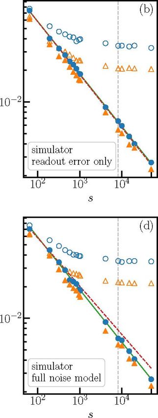
The derivation of the corresponding variances is Starting from an arbitrary single-qubit density
provided in Appendix B. operator
3.1 Measurement of a single Z operator
3.1.1 Prediction for the noisy expectation value
p = (1 + r • a)/2, (9)
For Q = 1 and arbitrary N, the noise-free oper
ator Zq gets replaced by the random noisy oper where r is a real vector with ||r|| < 1 and a is the
ator Zq, which can take the values vector containing the Pauli matrices, any quan
tum channel acting on the state p is an affine
• Zq with probability (1 - pq,0)(1 - Pq, 1),
linear map
• -1q with probability pq,o(1 - Pq,i),
• 1q with probability (1 - Pq,o)pq,i,
r ^ r' = Mr + c, (10)
• or - Zq with probability pq>0pq>1. where M is a 3 x 3 real matrix and c is a con
stant real vector [36]. In particular, a noise-free
Here, pq,b is the probability of flipping the projective measurement in the computational ba
qubit q given that it is in the state b = |0) or sis corresponds to a unital channel with M =
|1). For example, p3,0 is the probability of flip diag(0, 0,1) and c = 0. For an arbitrary pure
ping |0) ^ |1) for qubit 3. single-qubit state, \ß) = a\0) + ß\1), with den
Then, we obtain the noisy expectation EZq for sity operator
the random operator Zq ,
EZq = (1 - pq,0 - pq,1)Zq + (pq,1 - pq,0)1q, (8)
p= (11)
which reduces to Eq. (5) for pq,0 = pq>1 =: p.
As before, “expectation” here means the expec
tation with respect to the bit-flip probabilities,
which should not be confused with the quantum such a projective measurement yields the classi
mechanical expectation value (ß\ O \ß) of the op cal mixture pc = diag(\a\2, \ß\2).
erator O. The expectation EO is the expected
value (as an operator) for the noisy operator O, In case of a noisy measurement, the bit flips
while E (^\ O \ß) is the expected value for the change the classical state that one obtains after
noisy (quantum mechanical) expectation value the measurement. As discussed above, (i) with
(ß\ O \ß) of the operator O. probability (1 - p0)(1 - p1) we obtain the origi
nal state, (ii) with probability p0(1 - p1) the \0)
flips to a \ 1), (iii) with probability (1 - p0)p1 the
3.1.2 Density matrix description and visualization
\ 1) flips to a \ 0), and (iv) with probability p0p1
of measurement noise
both measurement outcomes flip. The resulting
For the single-qubit case it is instructive to ex classical state can be expressed as a convex linear
press our results in terms of density matrices. combination of the different outcomes
_________________________________________ I
a 2 0 0 0 1 0 ß 2 0
pc = 0 \ ß \ 2 (1 - p0)(1 - p1) + 0 1 p0(1 - p1) + 0 0 p1(1 - p0) + 0 \ a \ 2 p1 p0
= f (1 - p0 - p1) \ a \2 + p1 0 \
0 (1 - p0 - p1) \ ß \2 + p0 '
(12)
5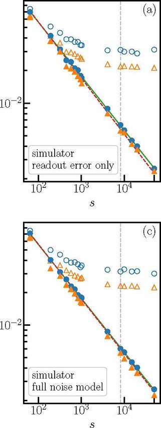
3.2 Measurement of Zq Z • • • Z Z1 operators
1-2P1 Going beyond Q = 1, we can now compute the
noisy expectations for arbitrary operators Zq Z
• • • Z Z1 with Q > 1 and arbitrary N. For this,
we assume that the expectations of the individual
-1 + 2p0 operators can be measured independently of each
other. In this case, the noisy expectation of the
tensor product Zq Z • • • Z Z1 equals the tensor
product of the individual noisy expectations,
Figure 2: Left panel: Possible range of Bloch vectors E (zq Z • • • Z Z^ = EZq z • • • Z EZ1. (15)
of the classical states pc obtained from a noise-free pro
jective measurement in the computational basis. Right Equation (15) can be proven by considering two
panel: Deformed range of Bloch vectors corresponding different noisy operators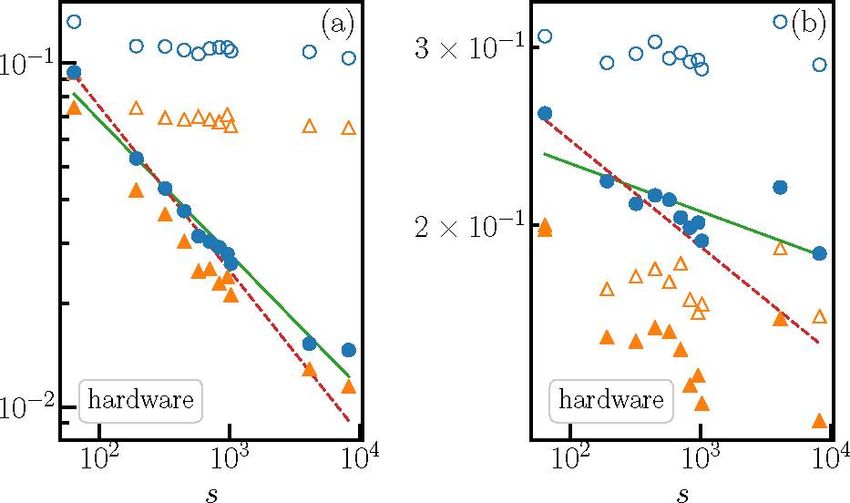
In order to construct the value of In particular, for O = Z2 U Z1, we obtain
Zq U • • • U Z-O in Eq. (17) inductively, it is
1
advantageous to choose the “lexicographic order" Z2 ® Z1 =
A for both the noise-free operators O G {1, Z}0Q Y(Z2)Y(Z1)
and the noisy operators O G {1, Z}0Q, Y (11)
1
Y (Z2)Y (Z1)
13 U 12 U 11 2213 U 12 U Z- (24)
Y (12)
12 U El
A13 U Z2 U 11 A 13 U Z2 U Zi Y(Z2)Y(Z1) v
(19)
AZ3 U 12 U 11 A Z3 U 12 U Zi Y(12)Y(11)
+ f7\ /-Z \ 12 U 11.
ZZ3 U Z2 U 11 A Z3 U Z2 U Zi A ... Y (Z2)Y (Z1)
This choice implies Oq U • • • U O1 A Zq U • • • U Z1 We can now evaluate Eq. (23) on an arbitrary
and will later ensure that the matrix w in Eq. (25) state \0) to find the bit-flip corrected expectation
is a lower triangular matrix, which is invertible values. For all O G {1, Z}0Q, we find
as long as none of its diagonal entries vanish. To
determine the matrix w, we need to generalize 01 O \0) = £ w-1OE (0| O\O . (25)
Eq. (17) to arbitrary noisy operators,
E (Öq U • •• U (51) In Fig. 3, we show the relative error for the bit
flip corrected expectation value of (0| Zq U • • • U
v(Oq\Oq')Oq u • • • u r(O1|O1)O1, Z1 0), as retrieved from histogram data using
oe{i,z}®Q Eq. (25), compared to the bit-flip free expecta
(20) tion value 01 Zq U • • • U Z1 \0)'-
where the coefficients r in front of the noise-free 101 Zq U • • • U Z1 \O - (0| Zq U • • • U Z1 |0>|
operators are now defined as
| 01 Zq ®---u Z110)1 .
forOq = Zq (26)
.— We also plot the standard deviation of this rela
r(Oq\oq) for Oq = 1q A Oq = 1q
tive error, alternatively to plotting the error bars.
for Oq = Zq A Oq = 1 q.
Figure 3 also contains a fit y(s) = Cs-a of the
(21) relative error in Eq. (26), where s is again the
number of shots, i.e., the number of (0 | Zq U
Using this definition, we can now define the ma
• • •UZ11 0) evaluations to produce the histogram.
trix w as
In particular, the fit indicates Monte-Carlo type
convergence a w 1/2 for Q G {1, 2, 3, 4}. Figure 3
w (O|C>) := n r(Oq Oq), has been generated using 4096 random states | 0)
q=1 (22) satisfying | (01 Zq U • • • U Z1 | 0) | > .25 to avoid
w := w dividing by small numbers when computing rel
O),oe{i,z}®Q
ative errors. For each \0) we randomly chose the
It is important to note that O A O implies bit-flip probabilities pq,b uniformly in (0.05,0.25).
O\O) =0. In other words, w is a lower tri
angular matrix and therefore invertible as long 3.3 Measurement of Zq U • • • U Z1 operators
as none of its diagonal entries vanish. The di assuming equal bit-flip probabilities
/ \
agonal entries are nq=1 r (Oq|Oq) and thus can
To compare the results of the previous two sub
only vanish if one of the y(Zq) vanishes, i.e., w is sections with the results obtained in Sec. 2, we
invertible as long as Vq : pq,0 + pq>1 = 1. If that now set all bit-flip probabilities pq,b = p to be
is the case, then we obtain the bit-flip corrected equal. For the case Q = 1, the expectation EZq
operators in Eq. (8) reduces to
(O)oe{i,Z}c« = w-1 (EO) }G0 . (23)
EZq = (1 - 2p)Zq, (27)
7
pressing them as linear combinations of oper
ators U*OU with O G {1,Z}0N on an N-
qubit machine, and by measuring each O inde
pendently (U being the transformation into the
Z basis). For example, if we are interested in
measuring Hzz = J^=1 ZiZi+1 with N = 3
qubits, then we generate independent histograms
for {^\ I3 ® Z2 ® Z1 |^), {^\ Z3 ® Z2 ® 11 |^), and
fy\ Z3 ® 12 ® Z1 \^), extract their expectation
values, and recover (^\HZZ \^) accordingly.
Alternatively, as we will discuss in the follow
Figure 3: Relative errors (blue dots) and standard devia
ing, we can measure the distribution of \^) and
tions (orange triangles) for the bit-flip corrected expecta obtain a histogram in terms of the computational
tion values of (^| Zq®- • •®Z1 |^), as retrieved from his basis {\j); j G N(hZ1, and (d) Z4®Z3Z0Z1.
be recovered from ^j pj (j\ H |j). For example, if
The average relative errors are fitted with a power law
we are interested in measuring the TI Hamilto
in the number of shots s, y(s) 1, the ex ware can be achieved by splitting the Hamilto
pectation in Eq. (15) reduces to nian into two sums of Pauli strings U^OkUk G
{1, X, Y, Z}0N, where multiple summands of the
E(Zq ••• Zi) = (1 - 2p)Q Zq ••• Z1, Hamiltonian are measured simultaneously. For
(28) example, both Hzz = J^=1 ZiZi+1 and Hx =
which yields Eq. (6) for Q = 2. This implies that h ^=1 Xi can be measured using bit-string dis
the matrix w in Eq. (22) becomes diagonal with tributions. Here, Hzz can be measured di
rectly by using the bit-string distribution of the
E(Oq »•••» (O1 ) = (1 - 2p)#Z(O) state \^) and Hx can be measured by using
(29)
X Oq »•••» O1, h ^iLi Zi and the bit-string distribution of the
where #Z(O) is the number of terms Oq = Zq state H®N \^), i.e., after applying a Hadamard
in the tensor product O = ON ® • • • ® O1. In gate H on each qubit. Hence, using the bit
particular, w is invertible as long as p = 1/2. string distribution, we can measure all the ZZ
We again observe in Eqs. (28) and (29) that the terms and all the X terms in the TI Hamilto
noisy expectations of arbitrary operators can be nian simultaneously. In other words, we are only
related to the true operators in a surprisingly required to measure two bit-string distributions
simple way, which requires no knowledge of the instead of measuring each of the 2N Pauli-terms
quantum hardware apart from the different bit separately. This allows for an efficient implemen
flip probabilities of the qubits. tation on the quantum hardware.
3.4 Measurement of general operators H from If we measure the distribution of |^), the mea
bit-string distributions of \^) surements of fy\ U
OU
* \^) comprising (^| H
are no longer independent. This has an impact
3.4.1 Prediction for the noisy expectation value
on the variance of measurement histograms, as
Our analysis of the bit-flip error above assumed we will discuss in Sec. 3.5. However, it has no
that we measure general operators H by ex impact on the expectation subject to bit flips,
8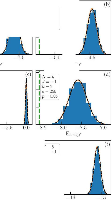
since linearity of the expectation value implies Thus, the bit-flip corrected noisy operator
—. . . . v-- . — . .
E (^\H \f) =E (^\^ KU * aOaUa \f) Hbfc := E Xa^aUa°aUa (36)
(30) a
= £ xaua (eo^ ua \f),
has the same Pauli-sum structure as the origi
nal operator H, changing only the coefficients.
which is precisely the expression we would ob
This is completely analogous to the independent
tain from summing the independently measured
measurement case. In both cases, if we have
operators Oa.
pq,o = pq,1, then we can correct for bit flips with
out additional cost to the quantum device.
3.4.2 Prediction for the bit-flip corrected operator
In order to correct for bit flips in this set 3.5 Impact of measurement choices
ting, we need to keep in mind that the gen
eral case requires measurements of all opera In general, we will extract the quantum mechani
tors O Oa (with respect to the lexicographic cal expectation of an operator by running the cir
order on {1,Z}0N) for all operators Oa in cuit preparing \^) followed by a projective mea
H = ^a XaU*OaUa. Hence, the histogram for surement in the computational basis a number
(^\ H \^) does not contain sufficient information. of times. As before, we refer to these repeti
However, we can use the classical bit-flip correc tions as the number of shots, s. Of course, these
tion method as discussed above to find coeffi shots are still subject to statistical fluctuations.
cients ua,o such that Hence, if we generate Mei histograms with s
shots each, we can generate a histogram from the
Oa = E ' -"O> (31) means extracted from each histogram. This will
O-O a
yield results as in Fig. 1 and Fig. 9. Using bit-flip
holds. Inserting this into H, we can express H as corrected operators as in Eq. (33), we can shift
the expected mean to coincide with the quantum
H = E XaU* E ^a,OEOUa. (32) mechanical expectation of the operator we wish
to measure. However, the variance of histogram
In other words, we can replace the operator H by means is then highly dependent on the measure
the bit-flip corrected noisy operator ment paradigm.
For illustration, let us consider the TI model
Hbfc := E XaUa E ^a,OOUa (33)
a O^Oa
Hti = J ZE Zj Zj+i+h ^N=1 Xj, which we will
measure on the ground state \^). The first step
and obtain is to compute the bit-flip corrected noisy Hamil
tonian HTI,bfc. For simplicity, we will assume all
E (^\H bfc \f) = H \f). (34)
bit-flip probabilities pq,b to coincide with some
value p. This yields
3.4.3 Prediction for equal bit-flip probabilities
N N
To compare our results to Secs. 2 and 3.3, let
HTI,bfc = Jp E Zj Zj+1 + hP E Xj (37)
us assume that the bit-flip probabilities pq,b sat
isfy pq,0 = pq,1 = pq, i.e., there is no difference
between p(\0) ^ \1)) and p(\1) ^ \0>) for each with Jp := J(1 — 2p)-2 and hp := h(1 — 2p)-1.
qubit, but this value might depend on the indi Of course, this process changes the variances.
vidual qubit. Then we obtain ua,O = 0 unless In particular, since Fig. 1 and Fig. 9 show his
O = Oa = Oa,N ® • • • ® Oa,i, for which we find tograms without the bit-flip correction, the pre
diction of variances in Fig. 1 (and Fig. 9 in the
W aOa : Wa n (1 - 2pq) , (35) Appendix) uses J and h instead of Jp and hp .
At this point, we need to decide upon the pre
where q ranges over all qubits satisfying Oa,q = cise way of measuring the Hamiltonian. Essen
Zq. For pq,b = p, this result agrees with Eqs. (5), tially, we have a spectrum of possibilities which
(6), and (28). contains three interesting cases:
9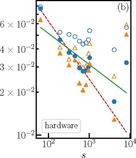
• Method 1: measure each Zj Zj+i and Xj in
Eq. (37) independently
• Method 2: measure the entire Hamiltonian
HTI,bfc in Eq. (37) from distributions of \fy)
measurements
H/T/77/n zi t T X—\ N r~7 r~7
• Method 3: measure Hzz := JPYj=1 ZjZj+1
and Hx := hp ^j=i Xj independently from
distributions of \fy) measurements
Methods 1 and 2 are the two extremes dis
Figure 4: Contributions to the variance of histogram
cussed in Secs. 3.1-3.3 and Sec. 3.4, respectively, means for the bit-flip corrected TI Hamiltonian in
whereas Method 3 is a reasonable compromise. Eq. (37) evaluated on the ground state of the “true” TI
In fact, Method 3 is precisely the method we used Hamiltonian in Eq. (51). The different bars correspond
for Fig. 1 and Fig. 9. Method 3 is also an exam to the the bit-flip (BF, blue) and quantum mechanical
ple that is closely related to implementations of (QM, orange) variance contributions for the three dif
quantum algorithms which are optimized for the ferent measurement methods. We used the parameters
N = 4, J = -1, h = 2, and pq,b = p = 0.05. All values
number of calls to the quantum device, i.e., im
are normalized by setting s = 1.
plementations in which only parts of an operator
can be measured simultaneously and both Meth
ods 1 and 2 are impractical to various degrees.
The variance of histogram means has two con evaluated the bit-flip corrected TI Hamiltonian
tributions: bit-flip variance and quantum me HTI,bfc = Jp Y,j=i Zj Zj + 1 + hp ^j=i Xj with
chanical variance. These contributions for each equal bit-flip probabilities pq,b = p = 0.05 on
of the three methods are shown in Fig. 4. The the ground state of the “true” TI Hamiltonian
derivation of these variances can be found in Ap Hti = J Ef=1 Zj Zj+i + h j Xj. For small
pendix B; in particular, Fig. 4 shows Eq. (77), values of p, we can interpret the bit-flip correc
Eq. (79), and Eq. (82). To remove the depen tion as a small perturbation to the original op
dence on the number of shots per histogram, all erator. Hence, the ground state of HTI is close
variances are multiplied by the number of shots to an eigenstate of HTI,bfc and thus the quantum
s, i.e., all values in Fig. 4 correspond to the nor mechanical contribution to the variance is small.
malization s = 1. For intermediate methods, such as Method 3,
It is interesting to note that not only the full it is generally difficult to predict the different
variance varies in magnitude but also the relative contributions to the variance using similar argu
contribution from bit flips and quantum mechan ments as above. Depending on the practical lim
ics is vastly different between the three methods. itation of any given implementation, it will be
If we compare the two extremes - Method 1 imperative to balance the different contributions
and Method 2 - we notice that for Method 1 to the variance with the number of quantum de
the bit-flip induced variance is small compared vice calls. For example, for the TI model, fewer
to the quantum mechanical variance, whereas quantum device calls per evaluation of the Hamil
for Method 2 the situation is reversed. Gener tonian introduce more covariance terms. In turn,
ically, this pattern is to be expected. Method 1 this requires more quantum device calls to ob
is likely to produce a much smaller bit-flip con tain the necessary statistical power if we aim to
tribution since all summands are measured inde extract a histogram mean with a required level
pendently. Meanwhile, measuring with Method of precision. Thus, this balancing act is highly
2 introduces O(4N) covariance terms, which problem specific. However, considering Method
vanish in Method 1 due to independent mea 3 for the TI model, it clearly shows that great
surements of summands. Moreover, concern care has to be taken when constructing an in
ing Method 2, we note that the quantum me termediate method if the aim is to reduce the
chanical variance vanishes upon evaluation on overall variance on a given budget of quantum
an eigenstate of the operator. In Fig. 4, we device calls.
104 Experimental results Thus we also explore the dependence of our re
sults on the number of shots s.
In order to demonstrate the experimental ap
plicability of our measurement error mitigation
4.1.1 Classical simulation of quantum hardware
method, we generate data on IBM quantum
hardware using the Qiskit software development To benchmark the performance of our correction
kit (SDK) [37]. To assess the performance of our procedure, we first simulate ibmqdondon [38] and
correction procedure, we first simulate the quan ibmq_burlington [39] classically. The Qiskit SDK
tum hardware classically using the noise models provides a noise model for each of the respective
for the different backends provided by Qiskit, be chips comprising various sources of error, includ
fore we proceed to the actual hardware. ing readout errors during the measurement pro
cess, which can be switched on and off individ
4.1 Single-qubit case ually. To begin with, we simulate the quantum
hardware incorporating the measurement errors
To begin with, let us focus on the simplest case only, subsequently we use the full noise model to
of a single qubit. In a first step, we determine see the effect of the various other errors. Our re
the bit-flip probabilities of the qubit. The prob sults for the mean and the standard deviation of
ability p0 can be easily obtained by measuring the absolute error as a function of s are shown in
the initial state |0) and recording the number of Fig. 5.
1 outcomes, while p1 requires preparing the state Focusing on the case with readout error only
|1) through applying a single X gate to the initial in Fig. 5(a) and 5(b), we see that correcting our
|0) state and recording the number of 0 outcomes. results according to Eq. (8) clearly reduces the
In order to account for statistical fluctuations, we mean and the standard deviation of the abso
repeat this procedure several times and average lute error in both cases. Without correction, the
over the bit-flip probabilities obtained for each
mean (standard deviation) of the absolute error
run (see Appendix C.1 for details). converges to a value around 8 x 10⁻¹ (9 x 10⁻¹),
After obtaining the bit-flip probabilities, we and increasing s beyond 1024 does not signifi
measure (^| Z for a randomly chosen |^). cantly improve the results. In particular, this
Starting from the initial state |0), we can prepare stagnation already happens for values of s be
any state on the Bloch sphere by first applying low the maximum one possible on real hardware,
a rotation gate around the £-axis followed by a hence showing that the readout error severely
rotation around the z-axis. Hence, we choose the limits the precision that can be achieved. On
circuit the contrary, the corrected results show a signifi
Rx(00)- Rz(0i) cant improvement and a power-law decay of these
|0)
quantities with s. In particular, in the ideal,
c
completely noise-free case, performing a projec
in our experiments, where the angles 00, 01 are tive measurement on is nothing but sampling
both drawn uniformly from the interval [0,2n]. from a probability distribution, thus one would
Our measurement outcomes allow us to deter expect the mean error to decay as rc s-1/2. To
mine the noisy expectation value of Z, E(Z). check for that behavior, we can fit the same func
Subsequently, we can apply our correction pro tional form as in Sec. 3.2 to our data, the result
cedure using Eq. (8). To acquire statistics for ing exponents are shown in Tab. 1. Indeed, we
E(Z), we repeat the process for 1050 randomly recover a = 1/2, thus demonstrating that our
chosen and monitor the mean and the stan correction procedure essentially allows us to re
dard deviation of the absolute error cover the noise-free case.
. . .. —. .. ... ... . , Taking into account the full noise model in our
|W>| Z [^ measured M Z |readout error only first 4 points full range
ibmqJondon 0.519 0.501
ibmq_burlington 0.503 0.499
full noise model first 4 points full range
ibmqJondon 0.508 0.500
ibmq_burlington 0.459 0.503
Table 1: Exponents a obtained from fitting the power
law Cs-a to our simulator data for the mean absolute
error in Fig. 5 after applying the correction.
The only difference with respect to the classical
simulation is that s on those two devices is lim
ited to a maximum number of 8192. Figure 6
shows our results obtained on real devices.
Comparing our data for the chip imbqdondon
in Fig. 6(a) to the classical simulation of the
quantum hardware in Fig. 5(a) and Fig. 5(c),
we observe qualitative agreement for s < 1024.
Compared to the classical simulation of the quan
tum device, the mean value and the standard de
Figure 5: Mean value (blue dots) and standard devia viation of the absolute error are in general larger
tion (orange triangles) of the absolute error in Eq. (38) on the hardware. Correcting for the readout er
after applying the correction procedure (filled symbols) ror yields again a significant improvement and
and without it (open symbols) as a function of the num reduces the mean and the standard deviation of
ber of shots s. The different panels correspond to the absolute error considerably. As before, we can
data obtained by classically simulating a single qubit of
fit our data to a power law. While for a small
the quantum hardware ibmqJondon (left column) and
number of shots about s < 500 we observe again
ibmq_burlington (right column) including readout noise
only (upper row) and using the full hardware noise model
an exponent of about 1/2, for a larger number
(lower row). The solid green line corresponds to a power of measurements the curve for the corrected re
law fit to all our data points for the mean absolute error, sult starts to flatten out and the exponent ob
the red dashed line to fit including the lowest four num tained for fitting the entire range is considerably
ber of shots. The vertical gray dashed line indicates the smaller than 1/2 (see Tab. 2 for details). Since
maximum number of shots, 8192, that can be executed increasing s should decrease the inherent statisti
on the actual hardware.
cal fluctuations of the projective measurements,
and readout errors can be dealt with our scheme,
readout procedure. The mean and the standard this might be an indication that in addition to
deviation of the absolute error without any cor readout errors also other sources of noise play a
rection only approach marginally higher values significant role. Their effects cannot be corrected
than previously. Again, we observe a significant with our procedure and thus dominate from a
reduction of the mean and the standard deviation certain point on.
of the absolute error after applying the correction Looking at the results for imbq_burlington in
procedure, and a power law decay with s. Fit Fig. 6(b) and comparing them with the classical
ting a power law to our data yields once more simulation of the quantum hardware in Fig. 5(b)
exponents around 1/2 (see Tab. 1). and Fig. 5(d), we see that the discrepancies in
this case are more severe and the data is less
consistent. Applying our mitigation to the data
4.1.2 Quantum hardware
again yields an improvement, which is less pro
Our experiments can be readily carried out on nounced than in the case of imbqdondon. For
quantum hardware, and we repeat the same sim a small number of shots, the mean of the abso
ulations on ibmqJondon and ibmq_burlington. lute error after correction shows again roughly a
12chip name first 4 points full range
ibmqdondon 0.460 0.298
ibmq_burlington 0.405 0.217
Table 2: Exponents a obtained from fitting the function
Cs-a to our hardware data for the mean absolute error
in Fig. 6 after applying the correction.
ing the following circuit
|0>
Figure 6: Mean value (blue dots) and standard deviation
(orange triangles) of the absolute error in Eq. (38) after
|0>
applying the correction procedure (filled symbols) and
without it (open symbols) as a function of the number of
c
shots s. The solid green line corresponds to a power law where the angles 00,..., 03 are again random
fit to all our data points for the mean absolute error, the numbers drawn uniformly from [0, 2n], and the
red dashed line to fit including the lowest four number of final CNOT gate allows for creating entangle
shots. Different panels correspond to single-qubit data
ment between the two qubits. Analogous to the
obtained on quantum hardware (a) ibmqdondon and (b)
ibmq_burlington.
single-qubit case, we first simulate the quantum
hardware classically before we eventually carry
out our experiments on a real quantum device.
In both cases we measure the noisy expectation
power law decay. The exponent obtained from a value of Z20Z1, E(Z2®Zi), and apply Eq. (25) to
fit to our data in that range is smaller compared correct for noise caused by readout errors. Again,
to the one from our data from ibmqdondon (see we repeat the procedure for 1050 randomly cho
Tab. 2 for details). From s = 1024 on, the uncor sen sets of angles and compute the mean and the
rected data is already less consistent. Making use standard deviation of the absolute error
of our mitigation scheme still yields an improve
ment, however, the corrected results scatter sim 1 I i 1r-r r~r 1 i \ lit r~r r~r 1 i \ 1
| (^| Z2 0 Z ^measured- M Z2 ® Z\ Inexact I
ilarly to the original ones and do not follow the (39)
same power law as for a small number of shots,
as a fit to our data reveals. This suggests that as a function of the number of shots, s, with and
noise other than the one resulting from the mea without applying the mitigation scheme.
surement has a considerable contribution.
4.2.1 Classical simulation of quantum hardware
As for the single-qubit case, we use the Qiskit
SDK to classically simulate the chips imqdondon
4.2 Two-qubit case
and ibmq_burlington first with readout error only
and subsequently using the full noise model. Fig
Since our correction procedure is not limited to ure 7 shows our results for both cases.
the single-qubit setup, we can straightforwardly Looking at Fig. 7(a) and Fig. 7(b), we see that
apply it to multiple qubits. To assess the per the two-qubit case with just readout error be
formance for that case, we repeat the same pro haves like the single-qubit case. Without apply
cedure we did previously but now for a circuit ing any correction, the mean and the standard
encompassing two qubits. Since we assume the deviation of the absolute error initially decrease
bit-flip probabilities pq,b (with q = 1, 2, b = 0,1) with increasing s, before eventually converging
of the qubits to be independent of each other, we to fixed values which are slightly higher than
apply the same procedure that we used to obtain for the single-qubit case (compare Fig. 5(a) with
the bit-flip probabilities in the single-qubit case, Fig. 7(a) and Fig. 5(b) with Fig. 7(b)). Applying
but this time for each qubit individually. the correction procedure, we can significantly de
Subsequently we prepare a two-qubit state us crease the values and observe again a power-law
13readout error only first 4 points full range
ibmqJondon 0.492 0.501
ibmq_burlington 0.522 0.503
full noise model first 4 points full range
ibmqJondon 0.446 0.238
ibmq_burlington 0.492 0.383
Table 3: Exponents a obtained from fitting the power
law Cs-a to our simulator data for the mean absolute
error in Fig. 7.
ber of shots. Considering the entire range of s
we study, the classical simulation of ibmqJondon
predicts that the data is not very well compati
ble with a power law. In contrast, our simulation
data for ibmq_burlington is still reasonably well
described by a power law, however with an expo
nent of 0.38 and thus considerably smaller than
1/2 (see Tab. 3 for details). Most notably, a com
parison between the results for classically simu
lating two qubits using the full noise model to
Figure 7: Mean value (blue dots) and standard devia
the single-qubit case in Fig. 5(c) and Figs. 5(d),
tion (orange triangles) of the absolute error in Eq. (39) we see that noise has a substantially larger ef
after applying the correction procedure (filled symbols) fect in the two-qubit case. This can be partially
and without it (open symbols) as a function of the num explained by the CNOT gate in the circuit, as
ber of shots s. The different panels correspond to the the error rates for two-qubit gates are in general
data obtained by classically simulating two qubits of much larger than for single-qubit rotations.
the quantum hardware ibmqJondon (left column) and
ibmq_burlington (right column) including readout noise
only (upper row) and using the full hardware noise model 4.2.2 Quantum hardware
(lower row). The solid green line corresponds to a power
law fit to all our data points for the mean absolute er For the two-qubit case, we can carry out the sim
ror, the red dashed line to fit including the lowest four ulations on real quantum hardware as well. Us
number of shots. The vertical gray dashed line indicates ing again imbqJondon and ibmq_burlington we
the maximum number of shots that can be executed on obtain the data depicted in Fig. 8.
the actual hardware.
Our results for ibmqJondon in Fig. 8(a) show
qualitative agreement with the classical simula
tion. Once more, we see that the mean and
decay with an exponent of 1/2 over the entire the standard deviation of the absolute error ob
range of s we study, as a fit to our corrected data tained on the hardware converge to higher val
reveals (see also Tab. 3). ues than the ones obtained from the simulation
Repeating the same simulations, but this time (compare Fig. 7(c) and Fig. 8(a)). Correcting
with the full noise model, yields the results in our data according to Eq. (25), the mean of the
Fig. 7(c) and Fig. 7(d). Comparing this to the absolute error and its standard deviation are sig
case with readout error only, we see a more pro nificantly reduced. Comparing the reduction to
nounced effect than in the single-qubit case. Ap the single-qubit case in Fig. 6, we observe that
plying the correction reduces the mean and the for the two-qubit case, the improvement is even
standard deviation of the absolute error still con larger. In particular, for our largest number of
siderably, nevertheless one can observe that data shots s = 8192, the mean and the standard de
after correction converges to a fixed value with viation of the absolute error are reduced by ap
increasing s. In particular, the power law decay proximately one order of magnitude. The cor
with a = 1/2 is only present for a small num- rected data is again well described by a power
14chip name first 4 points full range
ibmqJondon 0.478 0.390
ibmq_burlington 0.105 0.047
Table 4: Exponents a obtained from fitting the power
law Cs-a to our hardware data for the mean absolute
error in Fig. 8.
5 Discussion
After demonstrating the applicability of our mit
Figure 8: Mean value (blue dots) and standard deviation igation method to real quantum hardware, we
(orange triangles) of the absolute error in Eq. (39) after discuss our results here in greater detail. We
applying the correction procedure (filled symbols) and comment on the relation to previous works on
without it (open symbols) as a function of the number of
error mitigation and address how our scheme al
shots s. The solid green line corresponds to a power law
fit to all our data points for the mean absolute error, the lows for extensions beyond those. In particular,
red dashed line to fit including the lowest four number we discuss the inclusion of multi-qubit correla
of shots. Different panels correspond to two-qubit data tions and the generalization to other types of er
obtained on quantum hardware (a) ibmqJondon and (b) rors such as relaxation. Moreover, we address
ibmq_burlington. some questions regarding the practical implemen
tation such as the overhead costs introduced, pre
processing versus post-processing, and the possi
bility to do probabilistic error mitigation.
law. Fitting the first 4 data points, we obtain an 5.1 Comparison to previous work
exponent of 0.48. Using the entire range of s for One way to mitigate measurement errors that
the fit, the exponent only decreases moderately has been put forward in the literature (see, e.g.,
to 0.39 (see also Tab. 4), thus showing that the Ref. [37]) is to construct a linear map, which
readout error has still a significant contribution relates the observed measurement outcomes for
to the overall error. each computational basis state to the state that
was actually prepared. To this end, one prepares
Turning to our results for ibmq_burlington in all computational basis states \i), i = 0,..., 2N —
Fig. 8(b), we see that the data for this chip 1, on the quantum device and records the prob
is significantly worse. For one, the mean value abilities p^ of obtaining the computational basis
(standard deviation) of the absolute error with state \j) after a projective measurement. The
out applying any correction procedure is roughly linear map w = (pji)ij=-o now relates the ob
a factor 3 (2) larger than the one obtained on served probability distribution of basis states P
ibmqJondon. Applying the correction procedure in a noisy measurement to the ideal distribution
still yields an improvement, however, this time it P as P = wP. Thus, one can in principle obtain
is a lot smaller than for ibmqJondon, as a com the exact solution P from the observed results
parison between Fig. 8(a) and Fig. 8(b) shows. by inverting w and post-processing P. Obviously,
While for a small number of shots, the mean the method scales exponentially with N in terms
value of the absolute error after correction still of the number of measurements and memory re
shows a power law decay, albeit with an expo quirements. In addition, w can be singular and
nent a lot smaller than 1/2, for a large number a direct inversion might not be possible. Even if
of shots this trend stops, as fits to our data re w-1 exists, it is not guaranteed to be stochastic,
veal (see also Tab. 4). This behavior is giving an such that the result obtained might not be a valid
indication that for ibmq_burlington, the readout probability distribution.
error is not the dominant one, but rather other To overcome these shortcomings, it has been
errors have a significant contribution which can proposed to mitigate measurement errors by ex
not be corrected for using our scheme. pressing the error-corrected result in terms of a
15sum of noisy outcomes and combinations of bit in Appendix C. For example, while the single
flip probabilities [6, 33, 34]. This has first been qubit calibrations required measuring p(\j) | \k))
studied by Kandala et al. [6] for the case of single for j, k G {0,1}, the two-qubit calibrations
qubit Z-operator measurements. An extension of would require measuring p(\j) | |k)) for j, k G
this method has been provided by Yeter-Aydeniz {00,01,10,11}. Since we are interested in n-
et al. [33, 34] for multi-qubit Zq ® • • • ® Z1- local Hamiltonians with at most n-qubit inter
operators with expectation values measured from actions (see also the discussion in Sec. 5.6), the
bit-string distributions. Our approach provides calibration cost scales polynomially in the num
a novel and alternative proof for some of the re ber of qubits N, as no more than n qubits are
sults in Ref. [33, 34], which offers an implemen measured simultaneously. Indeed, the multi
tation beyond bit-string distributions and allows qubit calibration method requires the calibra
for several further generalizations, which are dis tion of (N) n-qubit systems with fixed n, which
cussed in the following subsections. In particu requires O(Nn) calibrations. Thus, incorporat
lar, our results can be extended to multi-qubit ing multi-qubit correlations into our mitigation
correlation errors (see Sec. 5.2), relaxation er scheme is straight-forward and requires relatively
rors (see Sec. 5.3), and probabilistic mitigation small overhead costs compared to previous ap
schemes (see Sec. 5.4). Moreover, while pre proaches.
vious results all rely on post-processing of the
error mitigation scheme, our method allows for
5.3 Extension to relaxation errors
pre-processing as well. Thus, it can be read
ily integrated into hybrid quantum-classical al Our method of replacing noisy operators with
gorithms, such as the variational quantum eigen- random operators that model the noise behavior,
solver (VQE) (see Sec. 5.5). as presented in Sec. 3, can in principle be gener
alized to other types of errors on noisy quantum
5.2 Inclusion of multi-qubit correlations computers. For example, if we wish to measure
the operator Z and consider the relaxation error
In our paper, we have assumed for simplicity that T1 (decay of |1) to |0)) [37], then we have a prob
there are no multi-qubit correlations in multi ability distribution of measuring Z (not yet de
qubit Zq ® - -® Zi-operator measurements. This cayed) and 1 (decayed). Hence, the measurement
is because most of the physically relevant Hamil outcome subject to the T1 error is described by
tonians only contain local interaction terms (see Z = p(t)Z + [1 — p(t)]1, where p(t) = exp (—T^
the discussion in Sec. 5.6). As such, the num
is the probability that |1) has not yet decayed.
ber of qubits for each multi-qubit Zq ® • • • ® Z1-
operator measurement is relatively small and the With our scheme of replacing noisy with ran
dom operators, this Ti error can be corrected
correlations are negligible.
as Z = pit) Z — 1~|p)t) 1. As such, our approach
However, as more qubits are measured simul
is generalizable to other types of errors beyond
taneously, multi-qubit correlations can become
measurement errors, and needs to be adapted ac
significant and have to be taken into account.
cordingly in order to correctly incorporate the
This has not been incorporated into the above
parameters underlying the specific type of error.
mentioned mitigation schemes [6, 33, 34] and,
to our knowledge, has only been addressed with
methods that are exponentially costly with the 5.4 Probabilistic implementation of the mea
number of qubits [40, 41]. surement error mitigation scheme
Our measurement mitigation scheme can eas
ily take multi-qubit correlations into account, The probabilistic description of the noisy opera
because the fundamental step of our approach tor naturally lends itself to a probabilistic imple
is the replacement of the operator to be mea mentation of the mitigation scheme.7 While de
sured with a probability distribution of opera terministic mitigation schemes require the mea
tors. Adding multi-qubit correlations into this surement of all mitigation terms, a probabilis
probability distribution is straight-forward and tic protocol allows for partial error mitigation
only requires multi-qubit calibration results sim
ilar to the single-qubit calibrations discussed 1 We thank Tom Weber for pointing this out to us.
16if the full mitigation is too costly. For exam each tensor product by a sum of up to 2N op
ple, if the corrected operator Z 0 Z is given by erators, which already need to be measured for
a1Z 0 Z + a2Z 0 1 + a31 0 Z + a41 0 1 = the full Hamiltonian measurement. Thus, the re
A(piSiZ0 Z+ p)2S2Z 01 + P3S3I 0 Z+ P4S4I 01) placement only changes the coefficients of these
with A := \aj|, Sj := sgn(aj), pj := J^J-, and operators but does not incur any overhead on the
^j pj = 1, then we may randomly draw the op
quantum device. Moreover, Hamiltonians with
non-local interactions are likely to incur exponen
erator to measure; namely, As1Z 0 Z with proba
tial complexity already in the evaluation of the
bility pi, As2Z01 with probability p2, et cetera.
expectation value, thus making them unfeasible
This can be used on a single-operator measure
to measure, let alone error correct.
ment, commuting sets of operators, as well as on
the level of drawing random Hamiltonians. It can For n-local Hamiltonians, the individual Pauli
also be generalized to other types of errors, such terms do not act on all N qubits but on a given
as the inclusion of multi-qubit correlations. number Q < n < N of qubits, which is inde
pendent of the total number N of qubits. For
5.5 Pre-processing the mitigation scheme example, the Ising model, the Heisenberg model,
and the Schwinger model (after integrating out
All of the previously known measurement miti the gauge field, see, e.g., Refs. [42-45]) exhibit at
gation schemes rely on post-processing, that is, most two-qubit interaction terms and thus have
first measuring without taking the error into ac Q < n = 2. For our mitigation method, we
count and afterwards manipulating the obtained now need to replace each tensor product of the
data (see, e.g., Refs. [6, 33, 34, 37, 40, 41]). How Q non-identity Pauli matrices by up to 2Q op
ever, this is not always possible using “black box erators. For each Q < n, there are polynomi
subroutines", such as VQE routines provided by ally many of these terms, (Q), and we can es
SDKs. Such routines typically ask for the Hamil timate the total number using the upper bound
tonian to be passed as an argument and they will ^QYou can also read